Thermal Environment Prediction for Metro Stations Based on an RVFL Neural Network

1
School of Electronic Information Engineering, North China University of Technology , Beijing 100144, China
2
Beijing Urban Construction Design & Development Group Co. Ltd., Beijing 100088, China
3
School of Aviation Science and Engineering, Beihang University (BUAA), Beijing 100191, China
*
Author to whom correspondence should be addressed.
Algorithms 2018, 11(4), 49; https://0-doi-org.brum.beds.ac.uk/10.3390/a11040049
Submission received: 9 March 2018
/
Revised: 10 April 2018
/
Accepted: 11 April 2018
/
Published: 17 April 2018
(This article belongs to the Special Issue Advanced Artificial Neural Networks)
Abstract
:With the improvement of China’s metro carrying capacity, people in big cities are inclined to travel by metro. The carrying load of these metros is huge during the morning and evening rush hours. Coupled with the increase in numbers of summer tourists, the thermal environmental quality in early metro stations will decline badly. Therefore, it is necessary to analyze the factors that affect the thermal environment in metro stations and establish a thermal environment change model. This will help to support the prediction and analysis of the thermal environment in such limited underground spaces. In order to achieve relatively accurate and rapid on-line modeling, this paper proposes a thermal environment modeling method based on a Random Vector Functional Link Neural Network (RVFLNN). This modeling method has the advantages of fast modeling speed and relatively accurate prediction results. Once the preprocessed data is input into this RVFLNN for training, the metro station thermal environment model will be quickly established. The study results show that the thermal model based on the RVFLNN method can effectively predict the temperature inside the metro station.
1. Introduction
There are two common methods to establish a thermal model in a space: the distributed parameter method and the lumped parameter method. The distributed parameter model is usually established by numerical approximation and discretization using the finite element method. Studies in the literature [1,2] use the distributed parameter method to establish a heat transfer model, and to achieve the distribution and prediction of object temperature. However, this method has the disadvantages of high computational cost and slow solution process. The lumped parameter model was established for the thermal node network method. The method uses the lumped parameter idea, which equates the object to a thermal node with uniform internal properties. Because of its simple principle, this method has been widely used in the field of heat transfer modeling [3,4,5,6]. One branch of the lumped parameter method is the neural network method. In recent years, with the development of artificial intelligence technology, the Artificial Neural Network (ANN) method has gained more and more of the attention of scholars. The ANN possesses the advantage of strong nonlinear fitting ability. It has become the main research direction when building a heat transfer model. This modeling technology does not require much knowledge about process mechanics and requires only a sufficient amount of experimental data [7,8,9,10,11]. Recently, the ANN method has been used to establish the nonlinear heat transfer model and predict temperature trends. This method avoids the difficulty of developing accurate models due to complex thermal processes [12,13]. The authors proposed the use of cellular neural networks and Tree-Structure Ensemble General Regression Neural Networks (TSE-GRNNs) to establish a heat transfer model. However, the ANN training process with a backpropagation algorithm has the disadvantage of slow convergence and long learning time. In contrast, the Random Vector Functional Link Neural Network (RVFLNN) can overcome these shortcomings. The RVFLNN can fit any nonlinear function by a linear combination of basis functions, randomly assigning input weights and biases [14]. It uses the least-square method to train its output weights [15]. The training process does not require iteration. Hence, it has a great advantage over the traditional ANN in terms of learning speed [16].
This paper aims to use the RVFLNN to quickly establish a thermal environment model for a metro station. This presented modeling method tries to predict the change trend of the temperature accurately inside the metro station. The RVFL network prediction model is obtained by analyzing the measured data at specified points from inside a metro station. The data for the input layer include temperatures, the passenger flow, and the arrival frequency of metro vehicles. Finally, we show that relatively good prediction results for the metro station can be obtained using the presented thermal prediction method based on an RVFLNN.
2. Training Principle of the RVFLNN Model
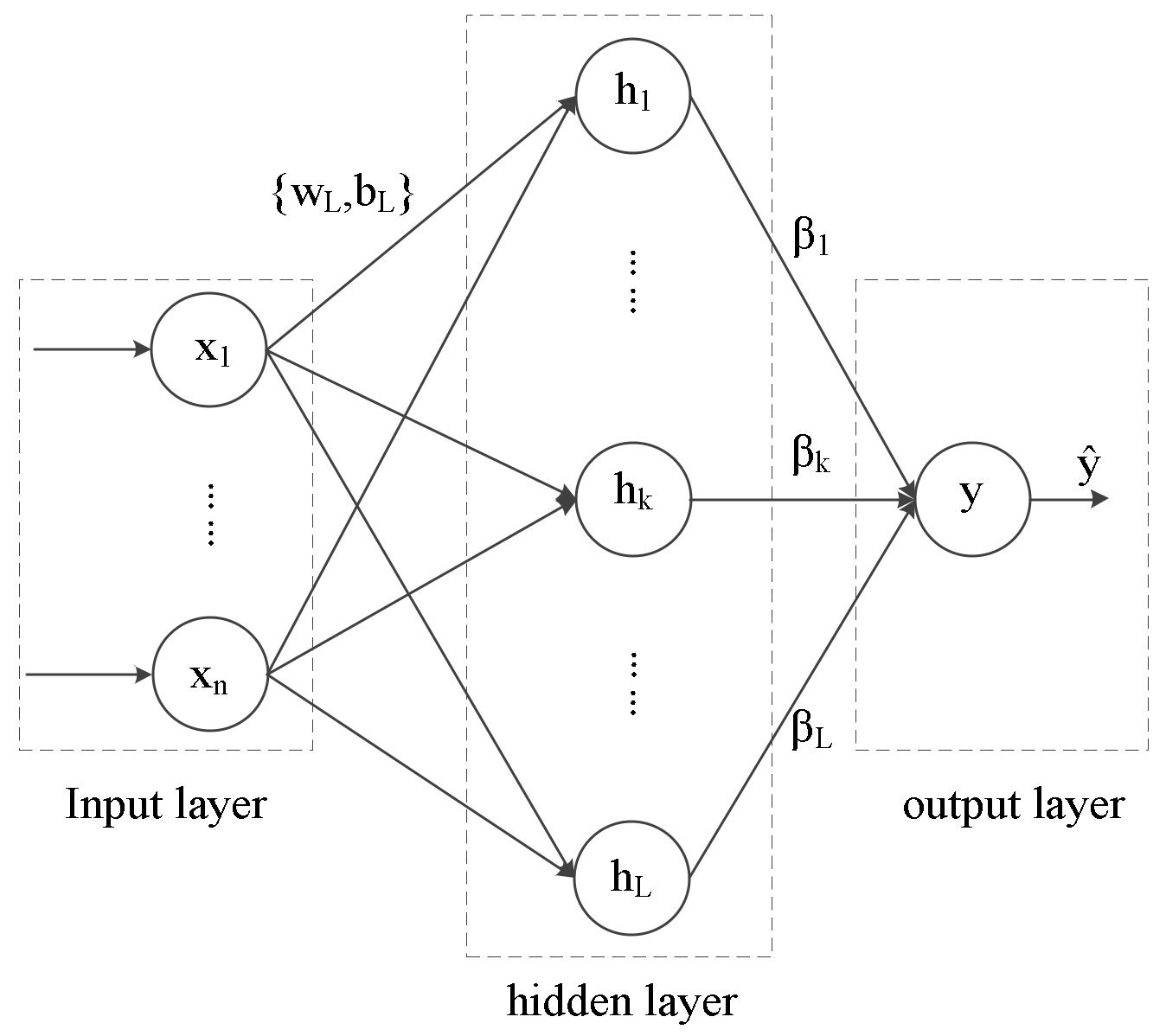
The RVFLNN has a good ability to quickly model a nonlinear process. Its basic structure is shown in Figure 1 [17].
(1) Input layer: is a given training set and is a -dimensional vector. WL and BL are weights and biases from the input layer to the hidden layer, with and . Here, d, N, and L are the dimension of input variables, the number of samples, and the number of hidden layer nodes, respectively. WL and BL are chosen in the beginning of the learning process, independently of the training data. In particular, WL and BL are chosen randomly from a predefined probability distribution in an RVFLNN. Hence, the input sets, weights, and biases of RVFLNN are as shown in Equations (1) and (2):
(2) Hidden layer: The purpose of the hidden layer is to establish an activation function, HL,N, for the hidden layer nodes. From Equation (3), each hl is a fixed nonlinear function known as a hidden function. In our paper, the sigmoid basis function is given by the following equation:
Finally, the hidden matrix, HN,L, is as shown in Equation (4):
(3) Output layer: A desired output, , is an N-dimensional vector. The output of an RVFLNN can be described as
Therefore, Equation (4) can be expressed in the form of the matrix
The output weights, , are the purpose of the training, so the learning problem can be formulated as minimizing both the training error and the output weight norm as follows:
where the factor is added for successive simplifications, and is the complexity coefficient. We obtain the well-known solution for :
where I is the identity matrix of proper dimensions to prevent numerical instabilities. Thus, the learning process can be completed using Equations (1)–(8) [18,19,20].
3. Measurement Process
3.1. Test Points in Metro Station
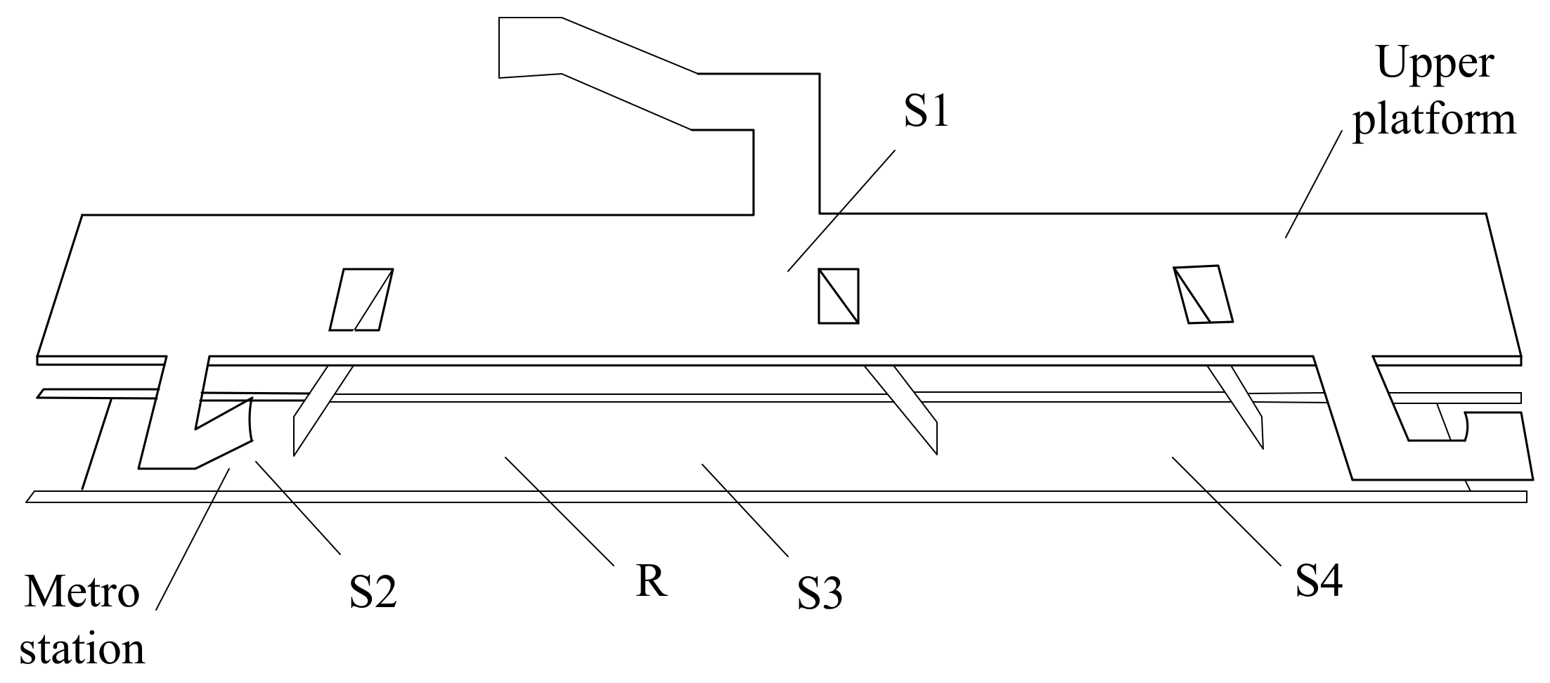
The measured metro station is an early station. Passengers can go down to the metro station from the upper platform by three staircases. The measured temperature points were distributed at four locations—S1, S2, S3, and S4 (Figure 2). S1 was at the upper platform and its temperature was very similar to the air supply temperature of the air conditioning system. S2, S3, and S4 were at the lower platform. Point R was the passenger flow monitoring point.
3.2. Data Acquisition and Processing
- (1)
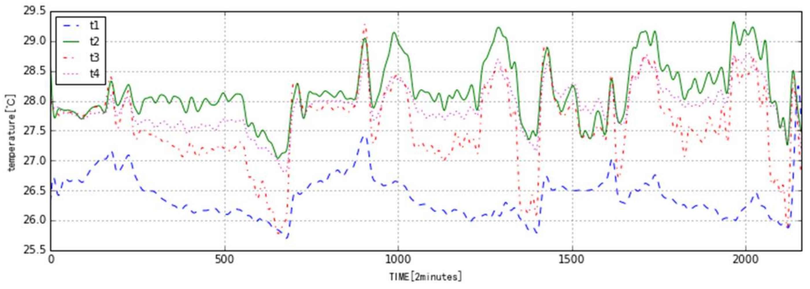
- The temperatures were monitored for 3 days and recorded every 2 min for a total of 2160 data points. T1, T2, T3, and T4 are temperatures at S1, S2, S3, and S4, respectively, as shown in Figure 3. They were processed from the primitive data with a Butterworth filter. The first 720 data points were measured on Sunday; the second and third lots of 720 data points were measured on Monday and Tuesday, respectively.
- (2)
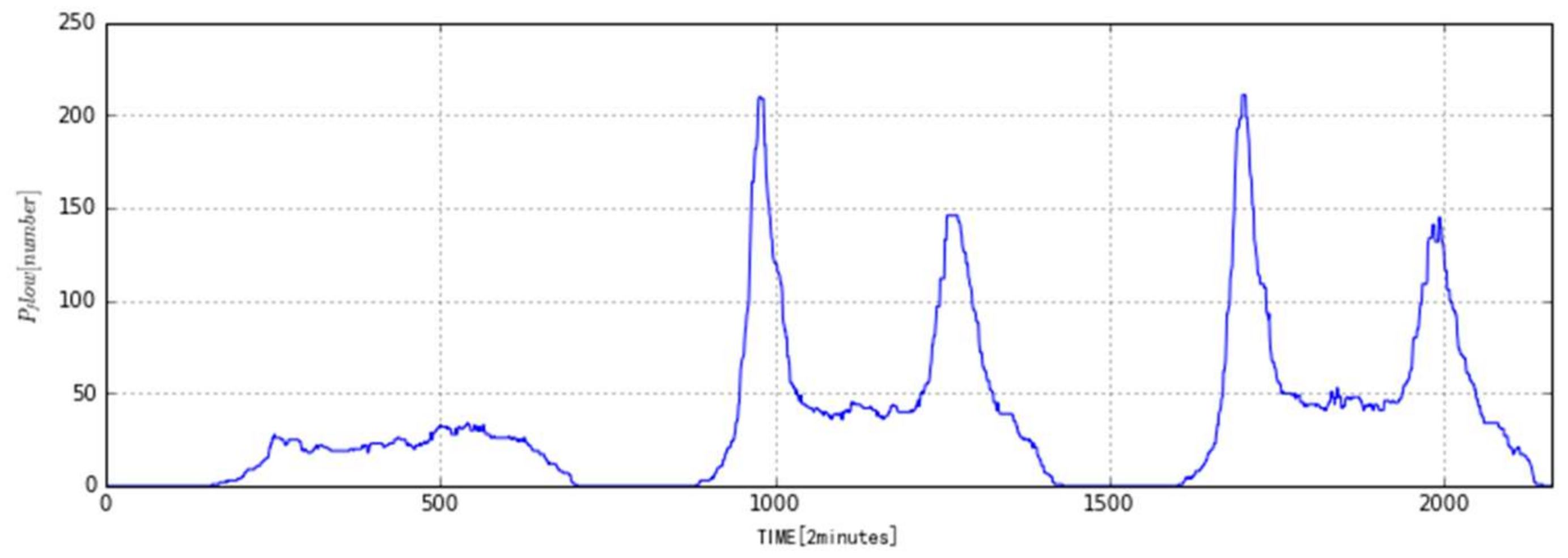
- The passenger flow monitoring point was at Point R. The number of passengers, Pflow, was monitored every two minutes. Figure 4 is the passenger flow curve after processing with median filtering. It is very obvious that the passenger flow data is very different between weekdays and weekends.
- (3)
- Since the metro arrival frequency, Ftrain, varies significantly with the time and the number of passengers, Figure 5 gives the change of Ftrain with time. It can be seen that Ftrain is obviously changed with the morning and evening rush hours. Ftrain is also different for weekdays and weekends.
3.3. Thermal Environment Model Based on an RVFLNN for a Metro Station
3.3.1. Model Input and Output
In practice, there are many parameters that will influence the climate, such as the air velocity, the relative humidity, diffused and direct solar radiation, and the latent thermal load due to the presence of people. Because of the limitations of our measuring instruments, only the parameters of temperature and relative humidity could be measured at S1, S2, S3, and S4. The measured data should be integrated with acquired air velocity and diffused/direct solar radiation data, which are very important for the evaluation of the local comfort [21,22,23]. In later analysis, we found that the relative humidity did not fluctuate greatly and remained within a certain range; hence, the relative humidity and temperature were not strongly correlated. The relative humidity was therefore not used to predict the temperature. In addition, the airflow velocity in the subway station is related to the frequency of the subway trains, and the radiation is related to the number of passengers. Therefore, our temperature prediction was finally based on the temperatures in different places, passenger flow, and metro arrival frequency.
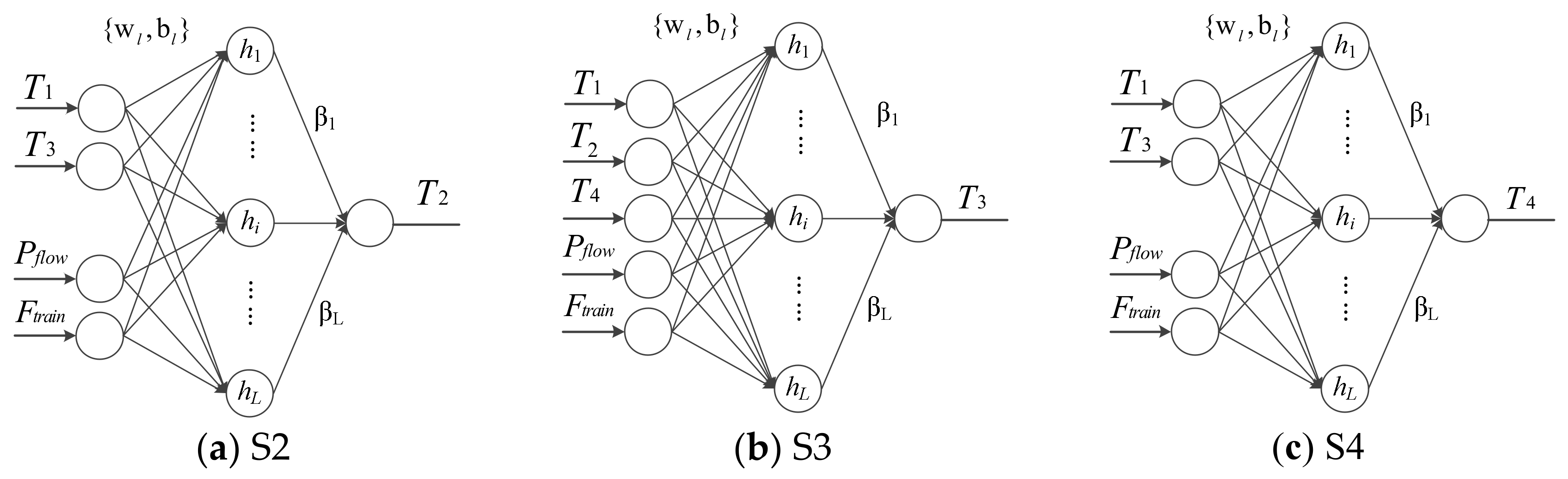
Because of the structure of the entire metro station, the air from S1 can provide cool air to the downstairs area and directly affect the temperature of S2, S3, and S4. At the same time, whenever the metro train arrives, the air flow change and the passenger flow all influence the temperature of S2, S3, and S4. The temperature of S1 affects those of S2, S3, and S4, but S2, S3, and S4 also influence each other. The whole space in the metro station was divided into three subspaces—S2, S3, and S4. In this paper, the thermal models for S2, S3, and S4 in the metro station were built separately. The parameters for the input layer of subspace S2 were determined to be T1, T3, Pflow, and Ftrain. For subspace S3, the parameters of the input layer were determined as T1, T2, T4, Pflow, and Ftrain. For subspace S4, the parameters of the input layer were determined as T1, T3, Pflow, and Ftrain. Therefore, T1, Pflow, and Ftrain are the common training input variables for S2, S3, and S4. The final structures of the traditional RVFL for the temperature models of T2, T3, and T4 are shown in Figure 6. The temperature prediction accuracy of S2 through S4 can be improved by establishing different neural network models.
Because the data were measured over three days—Sunday, Monday, and Tuesday—we see that the passenger flow and the metro arrival frequency are very different between weekdays and weekends. In order to obtain better prediction performance, the data from the first two days were used for the training. The data from the last day were used as the test data.
3.3.2. Input Normalization
The input data is normalized using the following equation:
where x’ denotes normalized data; x is the filtered data; xmin is the minimum value of x; and xmax is the maximum value of x.
The purpose of normalization is to allow input variables with different physical dimensions to be used together. In the meantime, the sigmoid function is used as a transfer function in the RVFLNN. The normalization can prevent neuron output saturation caused by excessive absolute values in the net input.
3.3.3. Build the Model
We established three neural network models. Every neural network step was the same.
The processes were carried out in the following steps:
Step 1: Divide training set, validation set, and test set.
The data were measured over three days—Sunday, Monday, and Tuesday. The total number of sample points is 2160. We used the first 1440 sample points as the training set, the next 360 sample points as the validation set, and the last 360 sample points as the test set.
Step 2: Set the number of neural network nodes.
From Figure 5, the input layer consists of 4, 5, and 4 neurons for T2, T3, and T4, respectively. The output layer has 1 neuron. The hidden layer was initially set to 20 hidden neurons. The hidden layer used sigmoid as the transfer function.
Step 3: Parameter initialization.
We set the regularization coefficient, λ, and randomly initialized w and b so that their mean value was 0 and the variance was 1. The range was [−1, 1].
Step 4: Training the RVFLNN.
The training data were input into the RVFLNN for training to get β. Then, the predicted data can be obtained from β.
Step 5: Training error and validation error evaluation and parameter adjustment.
The average relative error of the training data was calculated to evaluate the model accuracy. We adjusted the number of nodes in the hidden layer by comparing the training error and the validation error. When the training error continued to decrease and the validation error no longer decreased, but increased—that is, before overfitting—the network learning was stopped and the number of hidden layer nodes at this time was determined. Then, we minimized the training error by changing the regularization coefficient and the range of w and b. In the meantime, we stopped the algorithm.
Step 6: Test the RVFLNN performance.
The test data were used to evaluate the model performance based on the trained RVFLNN.
3.4. Results and Analysis
3.4.1. Effects of Training Parameters
With the RVFLNN, the predicted temperatures were made closer to the experimental temperatures by adjusting the number of hidden layer nodes, L, and the regularization coefficient, λ. In this paper, the model accuracy was evaluated using the average relative error, E. This can be calculated with the following equation:
where Texp,i and Tsim,i are the experimental data and prediction data, respectively; and N is the total number of sampling points. Table 1 shows the error versus the number of hidden layer nodes from 20 to 1000.
Etrain and Evalidation are the average relative errors of the training data and the validation data. After the initialization of RVFLNN parameters, the number of hidden layer nodes was adjusted. It can be seen from Table 1 that when the number of hidden layer nodes gradually increases from 20 to 1000, the training error continuously decreases. However, when the hidden layer nodes reach about 800, 200, and 100 for model S2, S3, and S4, respectively, the test error begins to increase or fluctuate. Therefore, we can draw a conclusion that the generalization effect of RVFLNN will be good when the respective number of hidden layer nodes for the three different RVFLNN models is 800, 200, and 100. Thus, we determined the number of hidden layer nodes.
For the RVFLNN, after determining the hidden layer nodes, we adjusted the regularization coefficients and the ranges of w and b. Taking the RVFLNN model S3 as an example, we can observe from Table 2 that no matter what the range of w and b is, the validation error will reach the minimum when the regularization coefficient is about 0.5 or 1. Moreover, the range of w and b has no significant effect on the minimum error. In conclusion, the system performance will be better when the regularization coefficient is finally determined as 1 and the range of w and b is [−1, 1].
3.4.2. Prediction Performance of Thermal Model Based on RVFLNN
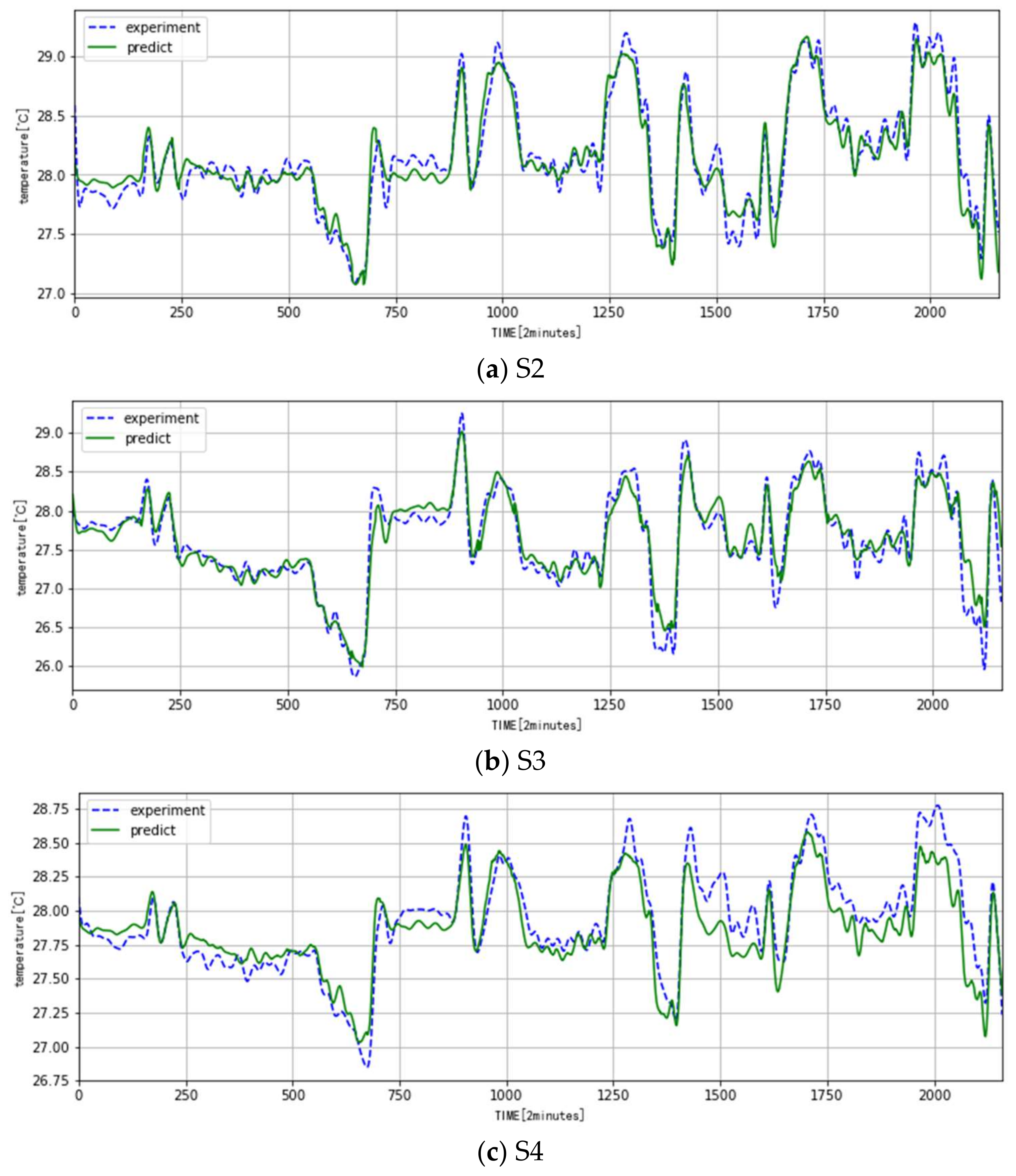
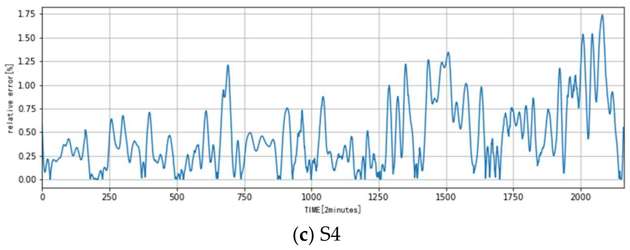
From the above analysis, the training parameters were finally determined—that is, the number of hidden layer nodes is 400 and the range of w and b is [−1, 1]. Hence, the thermal model based on RVFLNN was built with the above parameters. Figure 7 gives the comparison results of the prediction data with the experimental data. Figure 8 shows the relative error of the prediction and experimental data. The relative error can be calculated with the equation
where Texp,i and Tsim,i are the experimental data and the prediction data, respectively.
- (1)
- The temperature change in the metro station is influenced by many factors and its change rule is relatively complicated. The presented model based on the RVFLNN can reveal this rule very well: its fitting error and prediction error are both very small.
- (2)
- Comparison of the predicted data and experimental data shows that the maximum absolute error is about 0.4 °C and the maximum relative error is about 2.5%.
- (3)
The model accuracy has reached a good level and the presented modeling method can be used for future temperature prediction in metro stations.
4. Conclusions
In this paper, a thermal environment modeling method based on the RVFLNN was proposed for metro stations. By analyzing the interaction between the passenger flow, the metro arrival frequency, and temperature inside the station, the thermal relationship of input variables and output variables for the RVFLNN was carefully set up. The training time of the RVFLNN is very short, only about 0.002 s, which shows that the RVFLNN has fast nonlinear modeling ability. It can accurately learn the relationship between the input and output variables of a given data set, and achieve relatively high model accuracy. In model S2, the prediction error for all experimental conditions was within 0.25 °C, the relative error was kept within 1.4%, and the test error was within 4.124. In model S3, the prediction error for all experimental conditions was within 0.5 °C, the relative error was kept about 2.5%, and the test error was within 5.513. In model S4, the prediction error for all experimental conditions was within 0.5 °C, the relative error was kept within 1.75%, and the test error was within 6.925. In conclusion, satisfactory model accuracy can be obtained by using the RVFLNN.
Acknowledgments
This work was funded by the National Key R&D Program of China (2017YFB1201100).
Author Contributions
Qing Tian conceived and designed the experiments; Weihang Zhao performed the experiments; Yun Wei analyzed the data; Liping Pang contributed instrument; Weihang Zhao and Liping Pang wrote the paper.
Conflicts of Interest
The authors declare no conflict of interest.
References
- Ma, Z.; Wang, G.; Zhang, J.; Gu, Y.; Dai, L. Simulation and forecast of the grinding temperature based on finite element and neural network. J. Electron. Meas. Instrum. 2013, 2013, 1080–1085. [Google Scholar]
- Wu, B.; Cui, D.; He, X.; Zhang, D.; Tang, K. Cutting tool temperature prediction method using analytical model for end milling. Chin. J. Aeronaut. 2016, 29, 1788–1794. [Google Scholar]
- Deng, J.; Ma, R.; Yuan, G.; Chang, C.; Yang, X. Dynamic thermal performance prediction model for the flat-plate solar collectors based on the two-node lumped heat capacitance method. Sol. Energy 2016, 135, 769–779. [Google Scholar] [CrossRef]
- Le Tellier, R.; Skrzypek, E.; Saas, L. On the treatment of plane fusion front in lumped parameter thermal models with convection. Appl. Therm. Eng. 2017, 120, 314–326. [Google Scholar] [CrossRef]
- Underwood, C.P. An improved lumped parameter method for building thermal modeling. Energy Build. 2014, 79, 191–201. [Google Scholar] [CrossRef]
- Mezrhab, A.; Bouzidi, M. Computation of thermal comfort inside a passenger car compartment. Appl. Therm. Eng. 2006, 26, 1697–1704. [Google Scholar] [CrossRef]
- Tian, Z.; Qian, C.; Gu, B.; Yang, L.; Liu, F. Electric vehicle air conditioning system performance prediction based on artificial neural network. Appl. Therm. Eng. 2015, 89, 101–114. [Google Scholar] [CrossRef]
- Korteby, Y.; Mahdi, Y.; Azizou, A.; Daoud, K.; Regdon, G., Jr. Implementation of an artificial neural network as a PAT tool for the prediction of temperature distribution within a pharmaceutical fluidized bed granulator. Eur. J. Pharm. Sci. 2016, 88, 219–232. [Google Scholar] [CrossRef] [PubMed]
- Adewole, B.Z.; Abidakun, O.A.; Asere, A.A. Artificial neural network prediction of exhaust emissions and flame temperature in LPG (liquefied petroleum gas) fueled low swirl burner. Energy 2013, 61, 606–611. [Google Scholar] [CrossRef]
- Dhanuskodi, R.; Kaliappan, R.; Suresh, S.; Anantharaman, N.; Arunagiri, A.; Krishnaiah, J. Artificial Neural Network model for predicting wall temperature of supercritical boilers. Appl. Therm. Eng. 2015, 90, 749–753. [Google Scholar] [CrossRef]
- Kara, F.; Aslantaş, K.; Cicek, A. Prediction of cutting temperature in orthogonal maching of AISI 316L using artificial neural network. Appl. Soft Comput. 2016, 38, 64–74. [Google Scholar] [CrossRef]
- Starkov, S.O.; Lavrenkov, Y.N. Prediction of the moderator temperature field in a heavy water reactor based on a cellular neural network. Nucl. Energy Technol. 2017, 3, 133–140. [Google Scholar] [CrossRef]
- Wang, X.; You, M.; Mao, Z.; Yuan, P. Tree-Structure Ensemble General Regression Neural Networks applied to predict the molten steel temperature in Ladle Furnace. Adv. Eng. Inf. 2016, 30, 368–375. [Google Scholar] [CrossRef]
- Lgelnik, B.; Pao, Y.-H.; LeClair, S.; Shen, C.Y. The ensemble approach to neural-network learning and generalization. IEEE Trans. Neural Netw. 1999, 10, 19–30. [Google Scholar] [CrossRef] [PubMed]
- Rao, C.R.; Mitra, S.K. Generalized Inverse of Matrices and Its Applications; Wiley: New York, NY, USA, 1971. [Google Scholar]
- Wang, D.; Alhamdoosh, M. Evolutionary extreme learning machine ensembles with size control. Neurocomputting 2013, 102, 98–110. [Google Scholar] [CrossRef]
- Igelnik, B.; Pao, Y.H. Stochastic choice of basis functions in adaptive function approximation and the functional-link net. IEEE Trans. Neural Netw. 1995, 6, 1320–1329. [Google Scholar] [CrossRef] [PubMed]
- Scardapane, S.; Wang, D.; Panella, M.; Uncini, A. Distributed learning for Random Vector Functional-Link networks. Inf. Sci. 2015, 301, 271–284. [Google Scholar] [CrossRef]
- Pao, Y.H.; Park, G.H.; Sobajic, D.J. Learning and generalization characteristics of the random vector functional-link net. Neurocomputing 1994, 6, 163–180. [Google Scholar] [CrossRef]
- Alhamdoosh, M.; Wang, D. Fast decorrelated neural network ensembles with random weights. Inf. Sci. 2014, 264, 104–117. [Google Scholar] [CrossRef]
- Cannistraro, M.; Cannistraro, G.; Gestivo, R. The Local Media Radiant Temperature for the Calculation of Comfort in Areas Characterized by Radiant Surfaces. Int. J. Heat Technol. 2015, 33, 115–122. [Google Scholar] [CrossRef]
- Cannistraro, G.; Cannistraro, M.; Restivo, R. Smart Control of air Climatization System in Function on the Valuers of the Mean Local Radiant Temperature. Smart Sci. 2015, 3, 157–163. [Google Scholar] [CrossRef]
- Cannistraro, G.; Cannistraro, M.; Cannistraro, A. Evaluation of the Sound Emissions and Climate Acoustic in Proximity of ome Railway Station. Int. J. Heat Technol. 2016, 34, S589–S596. [Google Scholar]
Figure 1.
Random Vector Functional Link Neural Network (RVFLNN) structure.

Figure 2.
Metro station measuring point distribution.

Figure 3.
Processed temperature data.

Figure 4.
Processed passenger flow data.

Figure 5.
Metro train arrival frequency.

Figure 6.
Final structures of traditional RVFL.

Figure 7.
Comparison of predicted data with experimental data.

Figure 8.
Relative error of predicted and experimental data.


Table 1.
Effects of different numbers of hidden layer nodes on model performance.
| (a) S2 | |||||||||
| Number of Nodes | 20 | 50 | 100 | 200 | 300 | 400 | 600 | 800 | 1000 |
| Etrain | 3.687 | 3.435 | 3.404 | 3.438 | 3.333 | 3.284 | 3.271 | 3.235 | 3.224 |
| Evalidation | 4.532 | 4.201 | 4.144 | 4.119 | 4.067 | 3.991 | 3.972 | 3.910 | 3.941 |
| (b) S3 | |||||||||
| Number of Nodes | 20 | 50 | 100 | 200 | 300 | 400 | 600 | 800 | 1000 |
| Etrain | 4.657 | 4.391 | 4.294 | 4.162 | 4.126 | 4.122 | 3.958 | 3.930 | 3.920 |
| Evalidation | 6.011 | 5.807 | 5.490 | 5.452 | 5.528 | 5.613 | 5.487 | 5.502 | 5.494 |
| (c) S4 | |||||||||
| Number of Nodes | 20 | 50 | 100 | 200 | 300 | 400 | 600 | 800 | 1000 |
| Etrain | 3.229 | 2.866 | 2.791 | 2.720 | 2.695 | 2.660 | 2.629 | 2.600 | 2.585 |
| Evalidation | 6.880 | 6.760 | 6.714 | 6.824 | 6.773 | 6.846 | 6.763 | 6.821 | 6.773 |
Table 2.
Effects of different ranges of λ and ω, b on model performance.
| λ | ω,b ϵ [−0.5, 0.5] | ω,b ϵ [−1, 1] | ω,b ϵ [−2, 2] |
|---|---|---|---|
| Evalidation | Evalidation | Evalidation | |
| 0.05 | 5.554 | 5.596 | 5.917 |
| 0.1 | 5.557 | 5.586 | 5.667 |
| 0.5 | 5.485 | 5.464 | 5.632 |
| 1 | 5.478 | 5.455 | 5.447 |
| 5 | 5.491 | 5.630 | 5.626 |
| 10 | 5.826 | 5.725 | 5681 |
| 20 | 6.683 | 6.030 | 5.691 |
Table 3.
Test errors of the three RVFLNN models.
| S2 | S3 | S4 | |
|---|---|---|---|
| Etest | 4.124 | 5.513 | 6.925 |
© 2018 by the authors. Licensee MDPI, Basel, Switzerland. This article is an open access article distributed under the terms and conditions of the Creative Commons Attribution (CC BY) license (http://creativecommons.org/licenses/by/4.0/).
Share and Cite
MDPI and ACS Style
Tian, Q.; Zhao, W.; Wei, Y.; Pang, L. Thermal Environment Prediction for Metro Stations Based on an RVFL Neural Network. Algorithms 2018, 11, 49. https://0-doi-org.brum.beds.ac.uk/10.3390/a11040049
AMA Style
Tian Q, Zhao W, Wei Y, Pang L. Thermal Environment Prediction for Metro Stations Based on an RVFL Neural Network. Algorithms. 2018; 11(4):49. https://0-doi-org.brum.beds.ac.uk/10.3390/a11040049
Chicago/Turabian StyleTian, Qing, Weihang Zhao, Yun Wei, and Liping Pang. 2018. "Thermal Environment Prediction for Metro Stations Based on an RVFL Neural Network" Algorithms 11, no. 4: 49. https://0-doi-org.brum.beds.ac.uk/10.3390/a11040049
Note that from the first issue of 2016, this journal uses article numbers instead of page numbers. See further details here.