Automated Processing of fNIRS Data—A Visual Guide to the Pitfalls and Consequences


Abstract
:1. Introduction
1.1. Channel Exclusion Criteria
1.2. Motion Correction
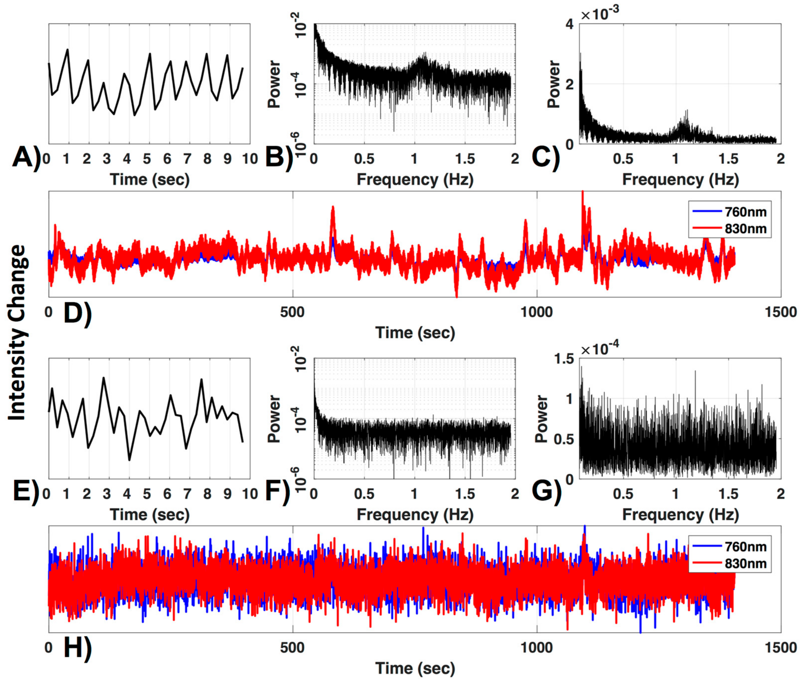
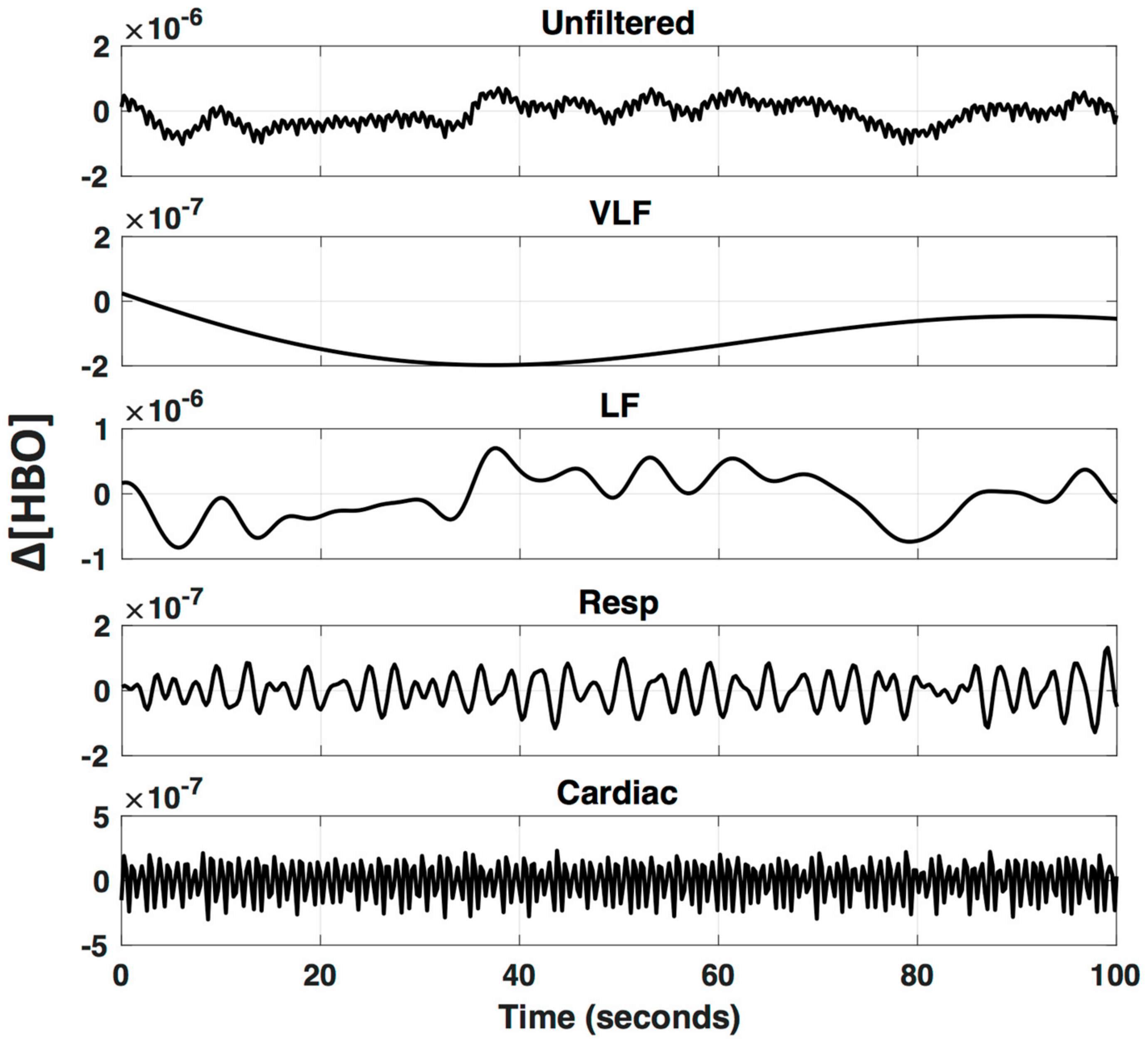
1.3. Filtering and De-Noising for Removal of Systemic Physiology
1.4. Statistical Evaluation of Task-Evoked Hemodynamics
2. Methods
2.1. Participants
2.2. Task
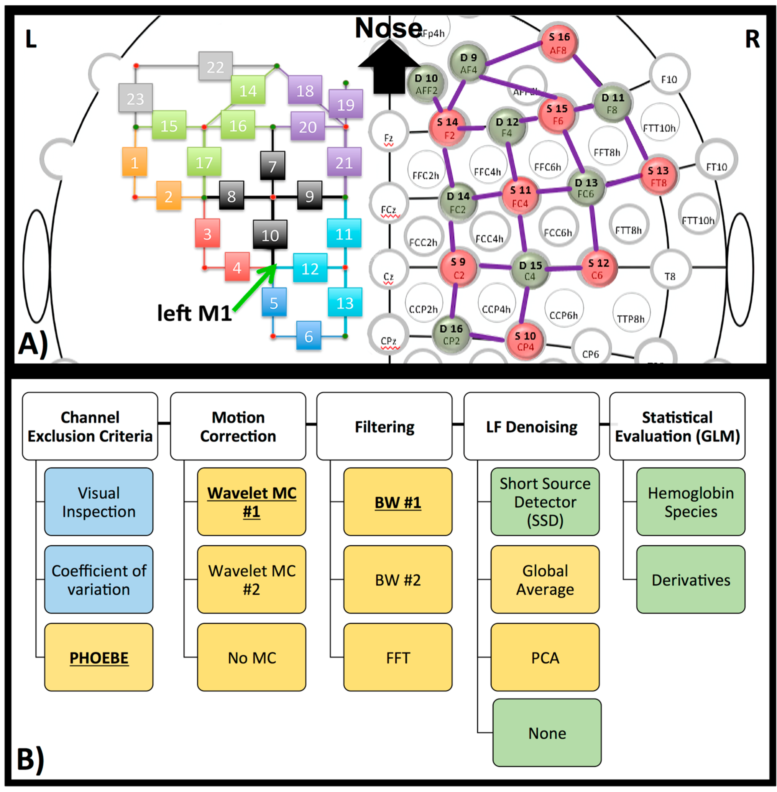
2.3. NIRS
2.4. Pre-Processing
2.4.1. Channel Exclusion Criteria
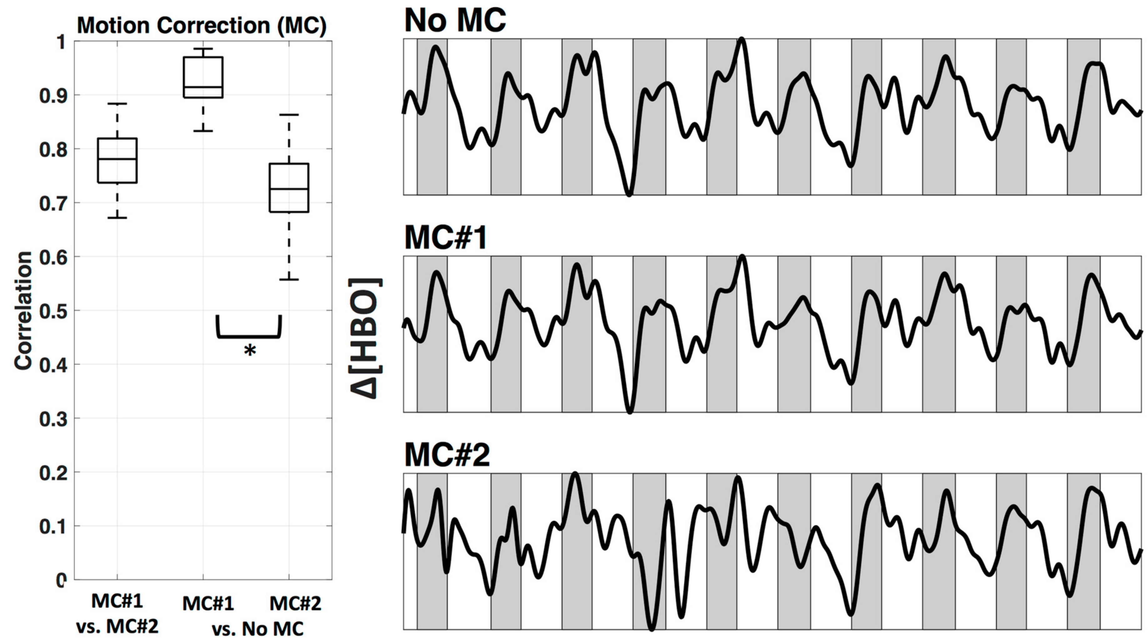
2.4.2. Motion Correction
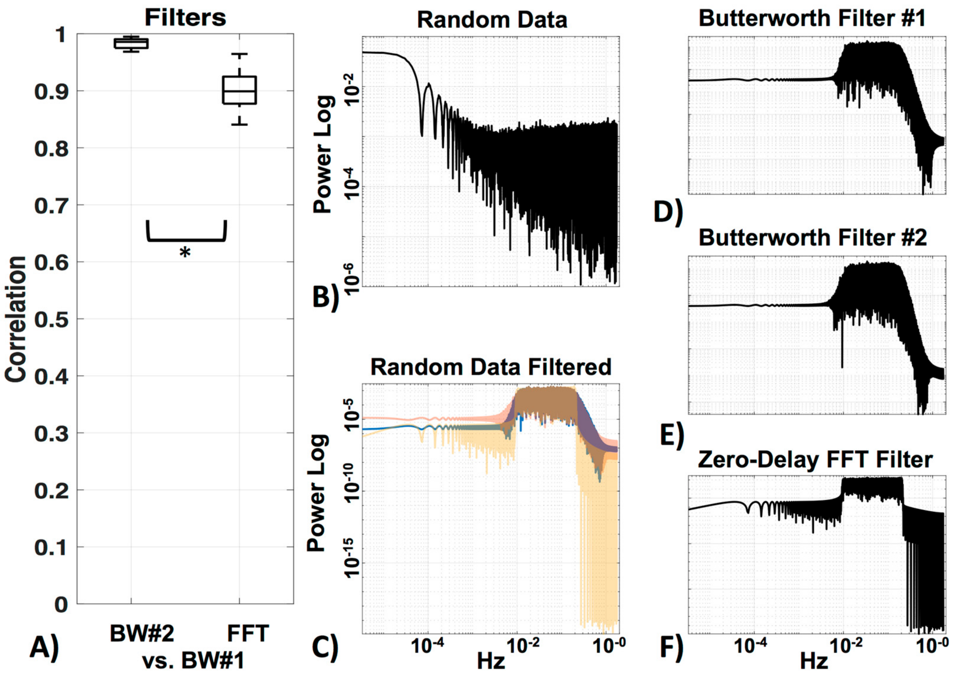
2.4.3. Filter
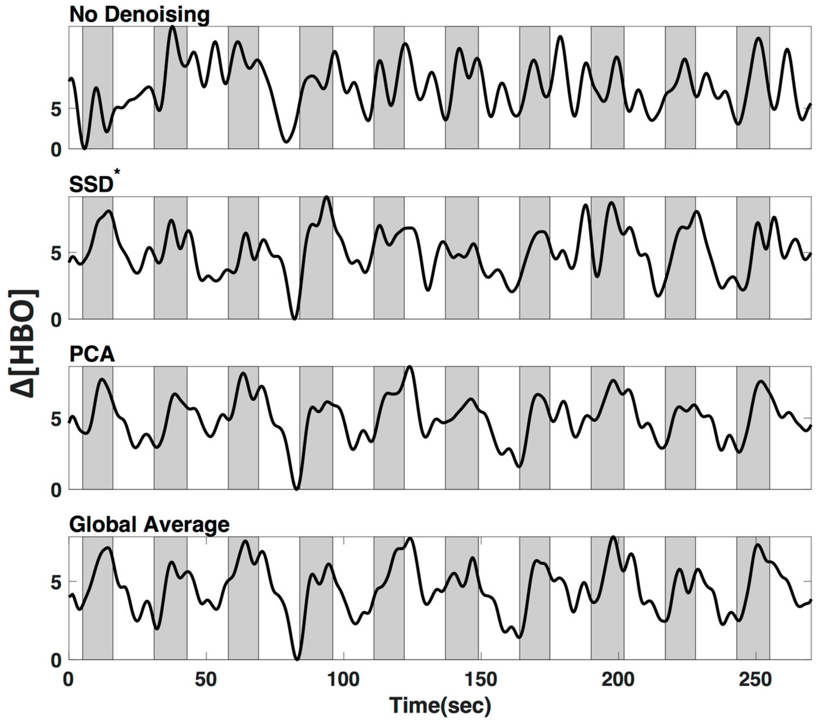
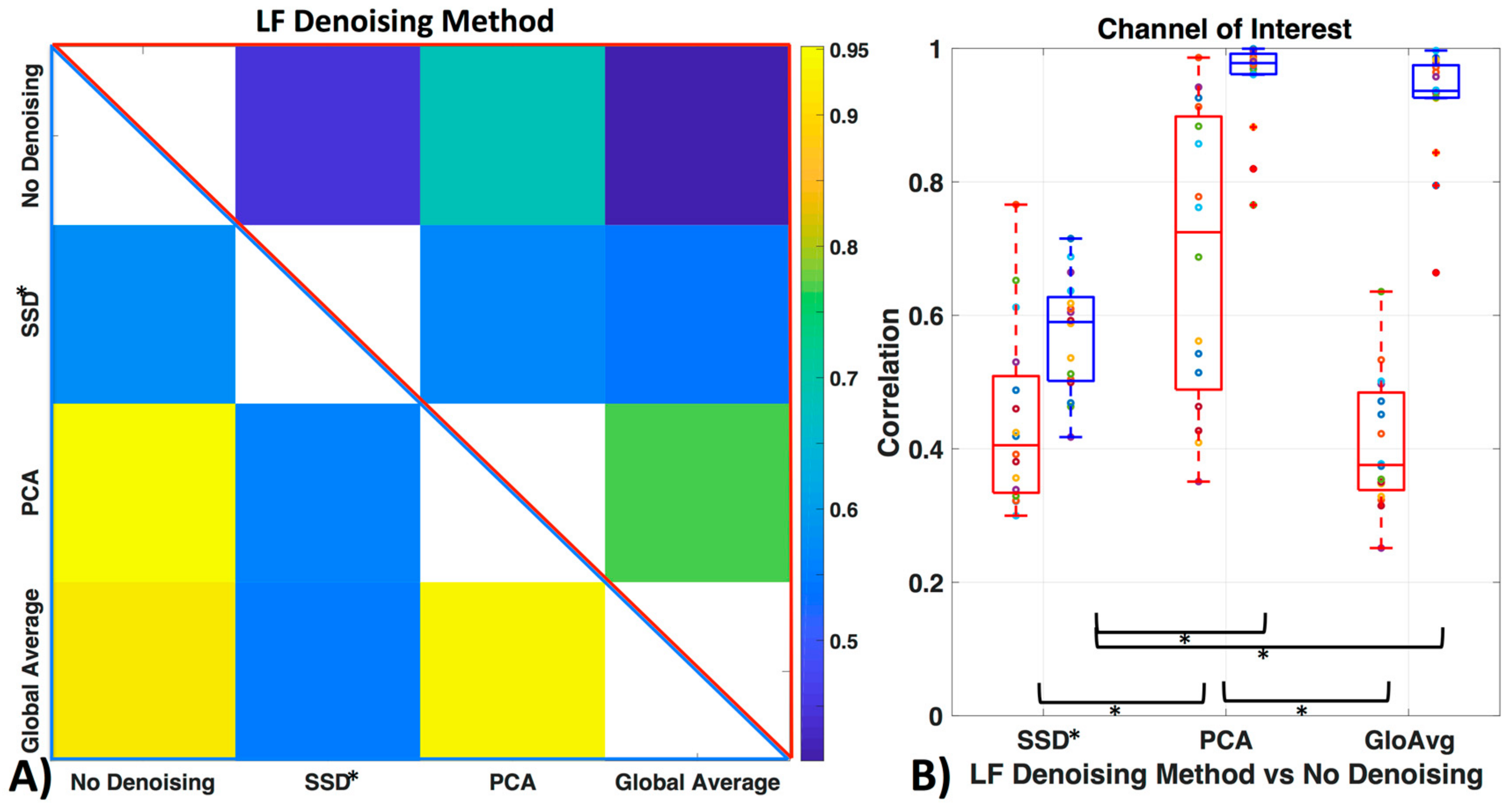
2.4.4. LF De-Noising Methods
2.5. Post-Processing
3. Results
3.1. Channel Exclusion Criteria
3.2. Motion Correction
3.3. Filter
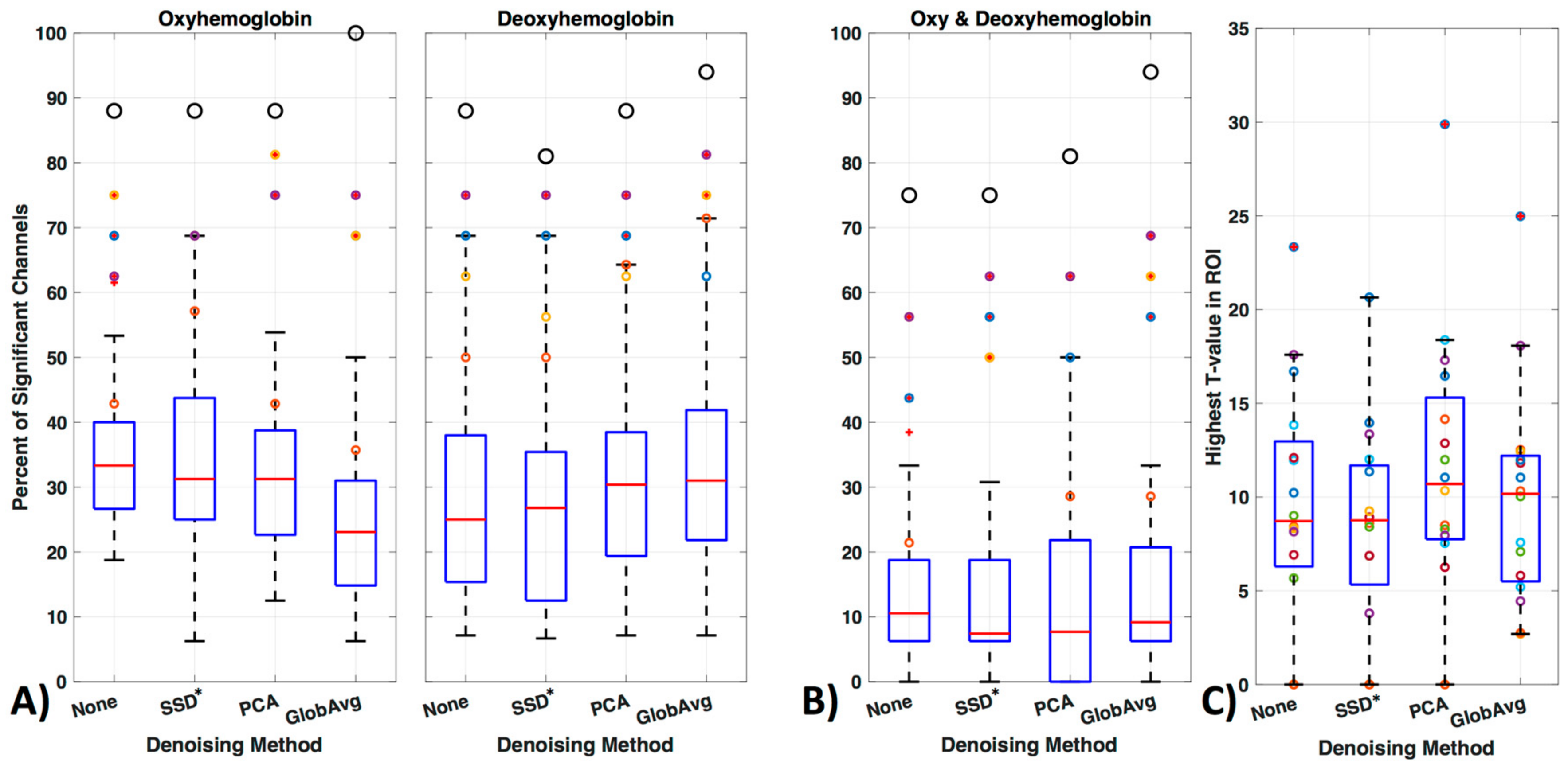
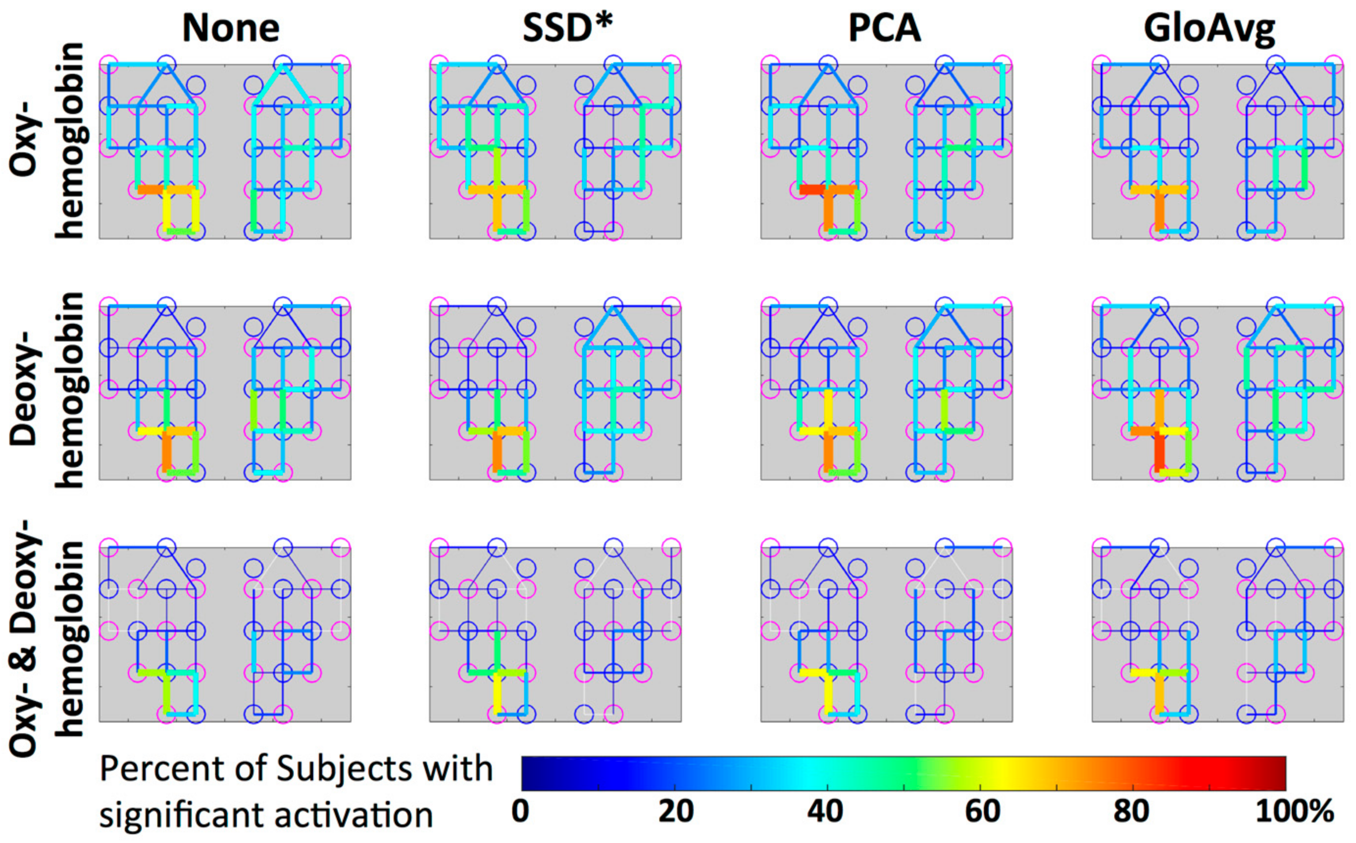
3.4. LF De-Noising Methods
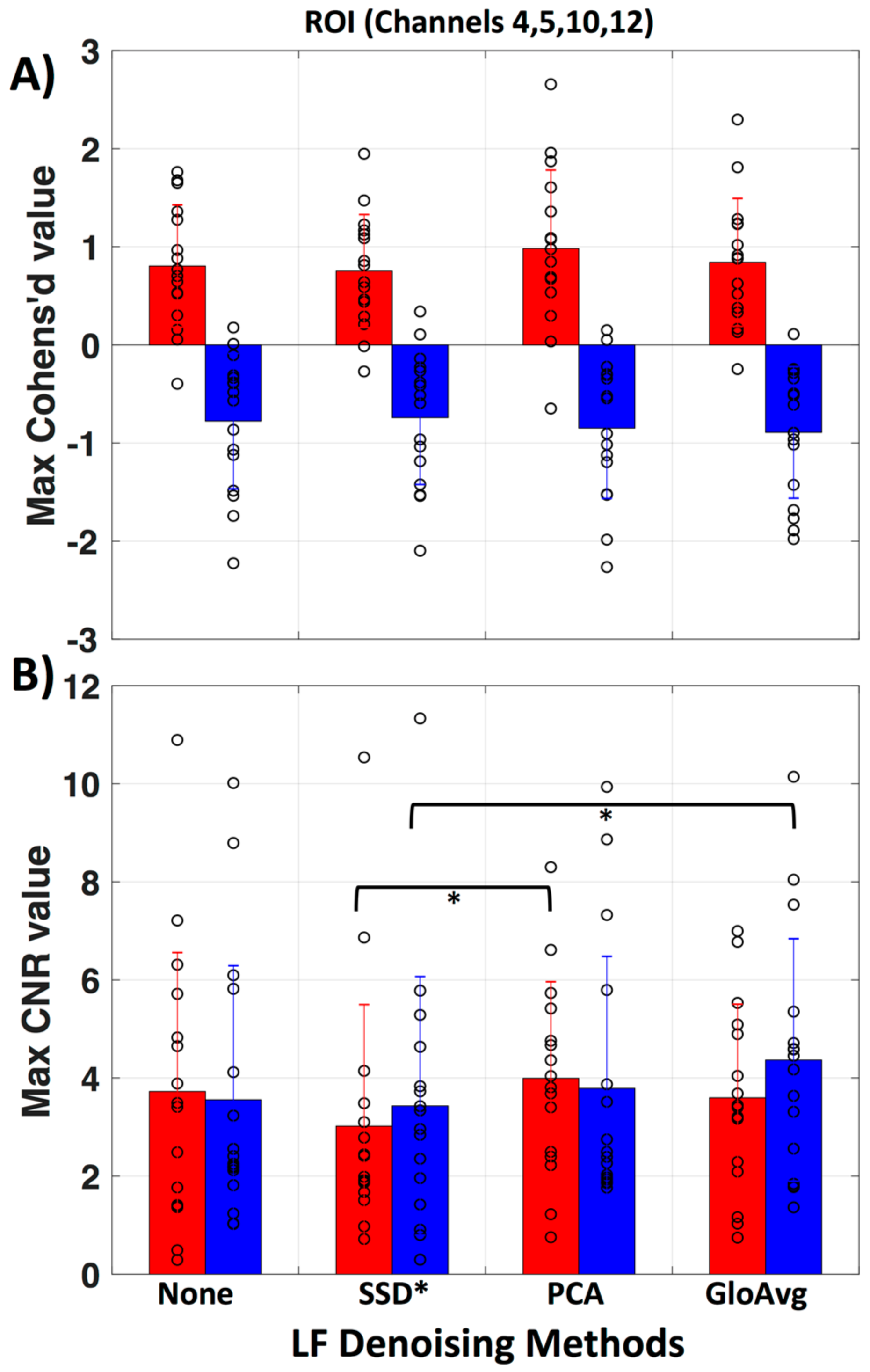
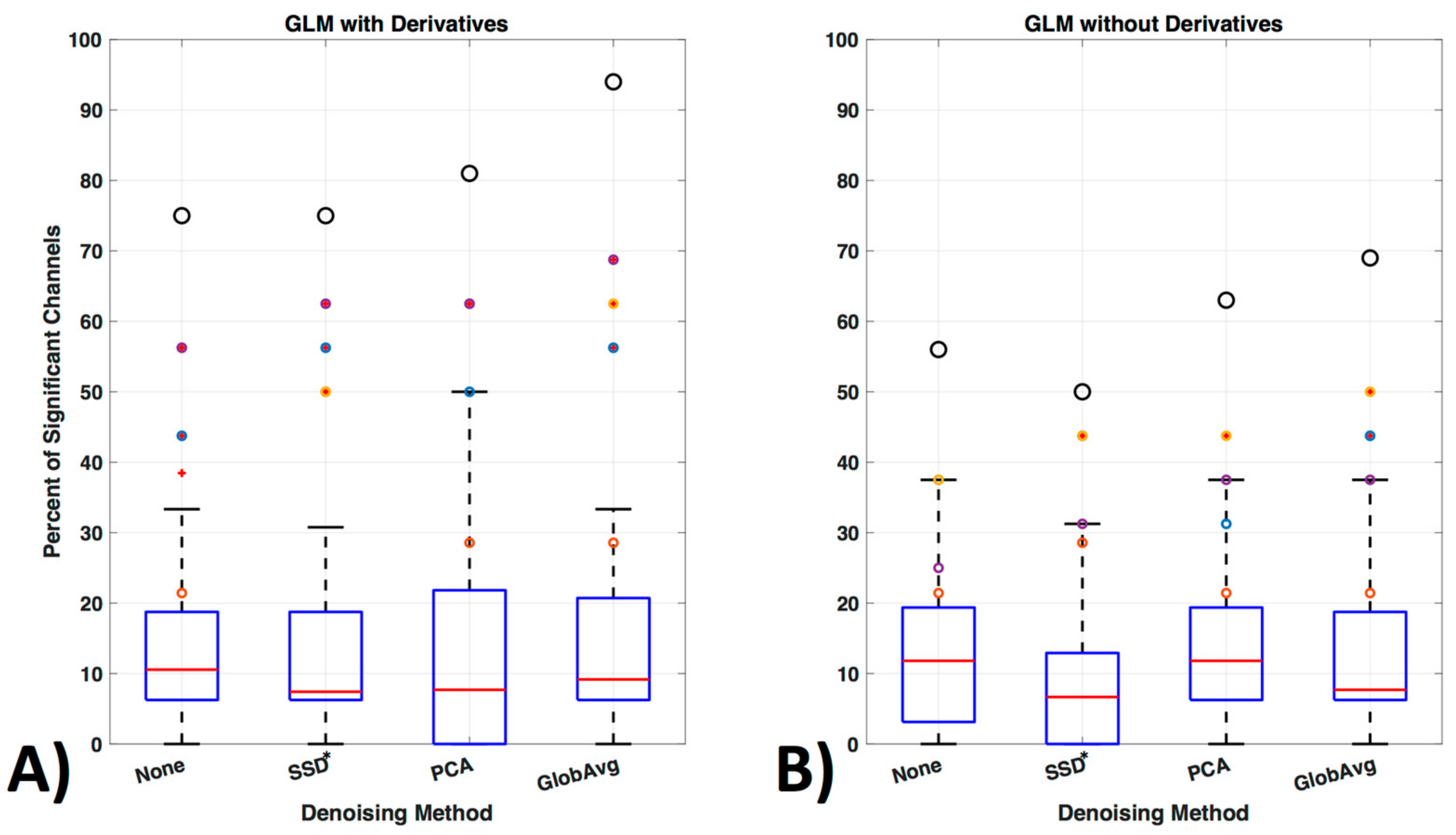
3.5. GLM Analysis
4. Discussion
4.1. Channel Exclusion
4.2. Motion Correction and Filter
4.3. LF De-Noising Methods
4.4. Hemoglobin
4.5. GLM
5. Conclusions
Author Contributions
Funding
Conflicts of Interest
Appendix A
References
- Boas, D.A.; Elwell, C.E.; Ferrari, M.; Taga, G. Twenty years of functional near-infrared spectroscopy: Introduction for the special issue. Neuroimage 2014, 85, 1–5. [Google Scholar] [CrossRef] [PubMed]
- Yucel, M.A.; Selb, J.J.; Huppert, T.J.; Franceschini, M.A.; Boas, D.A. Functional near infrared spectroscopy: Enabling routine functional brain imaging. Curr. Opin. Biomed. Eng. 2017, 4, 78–86. [Google Scholar] [CrossRef] [PubMed]
- Pfeifer, M.D.; Scholkmann, F.; Labruyere, R. Signal processing in functional near-infrared spectroscopy (fnirs): Methodological differences lead to different statistical results. Front. Hum. Neurosci. 2017, 11, 641. [Google Scholar] [CrossRef] [PubMed]
- Tachtsidis, I.; Scholkmann, F. False positives and false negatives in functional near-infrared spectroscopy: Issues, challenges, and the way forward. Neurophotonics 2016, 3, 031405. [Google Scholar] [CrossRef] [PubMed]
- Kirilina, E.; Yu, N.; Jelzow, A.; Wabnitz, H.; Jacobs, A.M.; Tachtsidis, I. Identifying and quantifying main components of physiological noise in functional near infrared spectroscopy on the prefrontal cortex. Front. Hum. Neurosci. 2013, 7, 864. [Google Scholar] [PubMed]
- Orihuela-Espina, F.; Leff, D.R.; James, D.R.; Darzi, A.W.; Yang, G.Z. Quality control and assurance in functional near infrared spectroscopy (fnirs) experimentation. Phys. Med. Biol. 2010, 55, 3701–3724. [Google Scholar] [CrossRef] [PubMed]
- Brigadoi, S.; Ceccherini, L.; Cutini, S.; Scarpa, F.; Scatturin, P.; Selb, J.; Gagnon, L.; Boas, D.A.; Cooper, R.J. Motion artifacts in functional near-infrared spectroscopy: A comparison of motion correction techniques applied to real cognitive data. Neuroimage 2014, 85, 181–191. [Google Scholar] [CrossRef] [PubMed]
- Huppert, T.J.; Diamond, S.G.; Franceschini, M.A.; Boas, D.A. Homer: A review of time-series analysis methods for near-infrared spectroscopy of the brain. Appl. Opt. 2009, 48, D280–D298. [Google Scholar] [CrossRef] [PubMed]
- Pollonini, L.; Bortfeld, H.; Oghalai, J.S. Phoebe: A method for real time mapping of optodes-scalp coupling in functional near-infrared spectroscopy. Biomed. Opt. Express 2016, 7, 5104–5119. [Google Scholar] [CrossRef] [PubMed]
- Cooper, R.J.; Selb, J.; Gagnon, L.; Phillip, D.; Schytz, H.W.; Iversen, H.K.; Ashina, M.; Boas, D.A. A systematic comparison of motion artifact correction techniques for functional near-infrared spectroscopy. Front. Neurosci. 2012, 6, 147. [Google Scholar] [CrossRef] [PubMed] [Green Version]
- Hu, X.S.; Arredondo, M.M.; Gomba, M.; Confer, N.; DaSilva, A.F.; Johnson, T.D.; Shalinsky, M.; Kovelman, I. Comparison of motion correction techniques applied to functional near-infrared spectroscopy data from children. J. Biomed. Opt. 2015, 20, 126003. [Google Scholar] [CrossRef] [PubMed]
- Molavi, B.; Dumont, G.A. Wavelet-based motion artifact removal for functional near-infrared spectroscopy. Physiol. Meas. 2012, 33, 259–270. [Google Scholar] [CrossRef] [PubMed]
- Scholkmann, F.; Spichtig, S.; Muehlemann, T.; Wolf, M. How to detect and reduce movement artifacts in near-infrared imaging using moving standard deviation and spline interpolation. Physiol. Meas. 2010, 31, 649–662. [Google Scholar] [CrossRef] [PubMed]
- Jahani, S.; Setarehdan, S.K.; Boas, D.A.; Yucel, M.A. Motion artifact detection and correction in functional near-infrared spectroscopy: A new hybrid method based on spline interpolation method and savitzky-golay filtering. Neurophotonics 2018, 5, 015003. [Google Scholar] [CrossRef] [PubMed]
- Obrig, H.; Neufang, M.; Wenzel, R.; Kohl, M.; Steinbrink, J.; Einhaupl, K.; Villringer, A. Spontaneous low frequency oscillations of cerebral hemodynamics and metabolism in human adults. Neuroimage 2000, 12, 623–639. [Google Scholar] [CrossRef] [PubMed]
- Diamond, S.G.; Perdue, K.L.; Boas, D.A. A cerebrovascular response model for functional neuroimaging including dynamic cerebral autoregulation. Math. Biosci. 2009, 220, 102–117. [Google Scholar] [CrossRef] [PubMed]
- Franceschini, M.A.; Fantini, S.; Thompson, J.H.; Culver, J.P.; Boas, D.A. Hemodynamic evoked response of the sensorimotor cortex measured noninvasively with near-infrared optical imaging. Psychophysiology 2003, 40, 548–560. [Google Scholar] [CrossRef] [PubMed]
- Kirilina, E.; Jelzow, A.; Heine, A.; Niessing, M.; Jacobs, A.; Heidrun, W.; Macdonald, R.; Bruehl, R.; Ittermann, B.; Bruehl, R.; et al. The physiological origin of task-evoked artifacts in functional near infrared spectroscopy. In Proceedings of the 17th Annual Meeting of the Organization for Human Brain Mapping, Quebec, QC, Canada, 26–30 June 2011. [Google Scholar]
- Naseer, N.; Hong, K.S. Fnirs-based brain-computer interfaces: A review. Front. Hum. Neurosci. 2015, 9, 3. [Google Scholar] [CrossRef] [PubMed]
- Caldwell, M.; Scholkmann, F.; Wolf, U.; Wolf, M.; Elwell, C.; Tachtsidis, I. Modelling confounding effects from extracerebral contamination and systemic factors on functional near-infrared spectroscopy. Neuroimage 2016, 143, 91–105. [Google Scholar] [CrossRef] [PubMed]
- Tong, Y.; Frederick, B.D. Studying the spatial distribution of physiological effects on bold signals using ultrafast fmri. Front. Hum. Neurosci. 2014, 8, 196. [Google Scholar] [CrossRef] [PubMed] [Green Version]
- Tong, Y.; Hocke, L.M.; Nickerson, L.D.; Licata, S.C.; Lindsey, K.P.; Frederick, B.D. Evaluating the effects of systemic low frequency oscillations measured in the periphery on the independent component analysis results of resting state networks. Neuroimage 2013, 76, 202–215. [Google Scholar] [CrossRef] [PubMed]
- Tong, Y.; Hocke, L.M.; Licata, S.C.; Frederick, B. Low-frequency oscillations measured in the periphery with near-infrared spectroscopy are strongly correlated with blood oxygen level-dependent functional magnetic resonance imaging signals. J. Biomed. Opt. 2012, 17, 106004. [Google Scholar] [CrossRef] [PubMed]
- Tong, Y.; Frederick, B. Concurrent fnirs and fmri processing allows independent visualization of the propagation of pressure waves and bulk blood flow in the cerebral vasculature. Neuroimage 2012, 61, 1419–1427. [Google Scholar] [CrossRef] [PubMed]
- Tong, Y.; Hocke, L.M.; Frederick, B. Isolating the sources of widespread physiological fluctuations in functional near-infrared spectroscopy signals. J. Biomed. Opt. 2011, 16, 106005. [Google Scholar] [CrossRef] [PubMed]
- Tong, Y.; Frederick, B.D. Time lag dependent multimodal processing of concurrent fmri and near-infrared spectroscopy (nirs) data suggests a global circulatory origin for low-frequency oscillation signals in human brain. Neuroimage 2010, 53, 553–564. [Google Scholar] [CrossRef] [PubMed]
- Scholkmann, F.; Kleiser, S.; Metz, A.J.; Zimmermann, R.; Mata Pavia, J.; Wolf, U.; Wolf, M. A review on continuous wave functional near-infrared spectroscopy and imaging instrumentation and methodology. Neuroimage 2014, 85 Pt 1, 6–27. [Google Scholar] [CrossRef] [PubMed] [Green Version]
- Tak, S.; Ye, J.C. Statistical analysis of fnirs data: A comprehensive review. Neuroimage 2014, 85 Pt 1, 72–91. [Google Scholar] [CrossRef] [PubMed]
- Saager, R.B.; Berger, A.J. Direct characterization and removal of interfering absorption trends in two-layer turbid media. J. Opt. Soc. Am. A Opt. Image Sci. Vis. 2005, 22, 1874–1882. [Google Scholar] [CrossRef] [PubMed]
- Yucel, M.A.; Selb, J.; Aasted, C.M.; Petkov, M.P.; Becerra, L.; Borsook, D.; Boas, D.A. Short separation regression improves statistical significance and better localizes the hemodynamic response obtained by near-infrared spectroscopy for tasks with differing autonomic responses. Neurophotonics 2015, 2, 035005. [Google Scholar] [CrossRef] [PubMed]
- Zhang, Y.; Brooks, D.H.; Franceschini, M.A.; Boas, D.A. Eigenvector-based spatial filtering for reduction of physiological interference in diffuse optical imaging. J. Biomed. Opt. 2005, 10, 11014. [Google Scholar] [CrossRef] [PubMed]
- Boas, D.A.; Dale, A.M.; Franceschini, M.A. Diffuse optical imaging of brain activation: Approaches to optimizing image sensitivity, resolution, and accuracy. Neuroimage 2004, 23 (Suppl. 1), S275–S288. [Google Scholar] [CrossRef] [PubMed]
- Carbonell, F.; Bellec, P.; Shmuel, A. Global and system-specific resting-state fmri fluctuations are uncorrelated: Principal component analysis reveals anti-correlated networks. Brain Connect. 2011, 1, 496–510. [Google Scholar] [CrossRef] [PubMed]
- Erdogan, S.B.; Tong, Y.; Hocke, L.M.; Lindsey, K.P.; deB Frederick, B. Correcting for blood arrival time in global mean regression enhances functional connectivity analysis of resting state fmri-bold signals. Front. Hum. Neurosci. 2016, 10, 311. [Google Scholar] [CrossRef] [PubMed]
- Friston, K.J.; Frith, C.D.; Turner, R.; Frackowiak, R.S. Characterizing evoked hemodynamics with fmri. Neuroimage 1995, 2, 157–165. [Google Scholar] [CrossRef] [PubMed]
- Ye, J.C.; Tak, S.; Jang, K.E.; Jung, J.; Jang, J. Nirs-spm: Statistical parametric mapping for near-infrared spectroscopy. Neuroimage 2009, 44, 428–447. [Google Scholar] [CrossRef] [PubMed]
- Uga, M.; Dan, I.; Sano, T.; Dan, H.; Watanabe, E. Optimizing the general linear model for functional near-infrared spectroscopy: An adaptive hemodynamic response function approach. Neurophotonics 2014, 1, 015004. [Google Scholar] [CrossRef] [PubMed]
- Pernet, C.R. Misconceptions in the use of the general linear model applied to functional mri: A tutorial for junior neuro-imagers. Front. Neurosci 2014, 8, 1. [Google Scholar] [CrossRef] [PubMed]
- Lindquist, M.A.; Meng Loh, J.; Atlas, L.Y.; Wager, T.D. Modeling the hemodynamic response function in fmri: Efficiency, bias and mis-modeling. Neuroimage 2009, 45, S187–S198. [Google Scholar] [CrossRef] [PubMed]
- Pinti, P.; Merla, A.; Aichelburg, C.; Lind, F.; Power, S.; Swingler, E.; Hamilton, A.; Gilbert, S.; Burgess, P.W.; Tachtsidis, I. A novel glm-based method for the automatic identification of functional events (aide) in fnirs data recorded in naturalistic environments. Neuroimage 2017, 155, 291–304. [Google Scholar] [CrossRef] [PubMed]
- Mathot, S.; Schreij, D.; Theeuwes, J. Opensesame: An open-source, graphical experiment builder for the social sciences. Behav. Res. Methods 2012, 44, 314–324. [Google Scholar] [CrossRef] [PubMed]
- Brigadoi, S.; Cooper, R.J. How short is short? Optimum source-detector distance for short-separation channels in functional near-infrared spectroscopy. Neurophotonics 2015, 2, 025005. [Google Scholar] [CrossRef] [PubMed]
- Gagnon, L.; Cooper, R.J.; Yucel, M.A.; Perdue, K.L.; Greve, D.N.; Boas, D.A. Short separation channel location impacts the performance of short channel regression in nirs. Neuroimage 2012, 59, 2518–2528. [Google Scholar] [CrossRef] [PubMed]
- Delpy, D.T.; Cope, M.; van der Zee, P.; Arridge, S.; Wray, S.; Wyatt, J. Estimation of optical pathlength through tissue from direct time of flight measurement. Phys. Med. Biol. 1988, 33, 1433–1442. [Google Scholar] [CrossRef] [PubMed]
- Zhao, H.; Tanikawa, Y.; Gao, F.; Onodera, Y.; Sassaroli, A.; Tanaka, K.; Yamada, Y. Maps of optical differential pathlength factor of human adult forehead, somatosensory motor and occipital regions at multi-wavelengths in nir. Phys. Med. Biol. 2002, 47, 2075–2093. [Google Scholar] [CrossRef] [PubMed]
- Duncan, A.; Meek, J.H.; Clemence, M.; Elwell, C.E.; Fallon, P.; Tyszczuk, L.; Cope, M.; Delpy, D.T. Measurement of cranial optical path length as a function of age using phase resolved near infrared spectroscopy. Pediatr. Res. 1996, 39, 889–894. [Google Scholar] [CrossRef] [PubMed]
- Scholkmann, F.; Wolf, M. General equation for the differential pathlength factor of the frontal human head depending on wavelength and age. J. Biomed. Opt. 2013, 18, 105004. [Google Scholar] [CrossRef] [PubMed] [Green Version]
- Zimeo Morais, G.A.; Scholkmann, F.; Balardin, J.B.; Furucho, R.A.; de Paula, R.C.V.; Biazoli, C.E., Jr.; Sato, J.R. Non-neuronal evoked and spontaneous hemodynamic changes in the anterior temporal region of the human head may lead to misinterpretations of functional near-infrared spectroscopy signals. Neurophotonics 2018, 5, 011002. [Google Scholar] [CrossRef] [PubMed]
- Pollonini, L.; Olds, C.; Abaya, H.; Bortfeld, H.; Beauchamp, M.S.; Oghalai, J.S. Auditory cortex activation to natural speech and simulated cochlear implant speech measured with functional near-infrared spectroscopy. Hear. Res. 2014, 309, 84–93. [Google Scholar] [CrossRef] [PubMed]
- Chiarelli, A.M.; Maclin, E.L.; Fabiani, M.; Gratton, G. A kurtosis-based wavelet algorithm for motion artifact correction of fnirs data. Neuroimage 2015, 112, 128–137. [Google Scholar] [CrossRef] [PubMed]
- Hocke, L.M.; Tong, Y.; Lindsey, K.P.; de B Frederick, B. Comparison of peripheral near-infrared spectroscopy low-frequency oscillations to other denoising methods in resting state functional mri with ultrahigh temporal resolution. Magn. Reson. Med. 2016, 76, 1697–1707. [Google Scholar] [CrossRef] [PubMed]
- Germon, T.J.; Evans, P.D.; Barnett, N.J.; Wall, P.; Manara, A.R.; Nelson, R.J. Cerebral near infrared spectroscopy: Emitter-detector separation must be increased. Br. J. Anaesth. 1999, 82, 831–837. [Google Scholar] [CrossRef] [PubMed]
- Zhang, Q.; Strangman, G.E.; Ganis, G. Adaptive filtering to reduce global interference in non-invasive nirs measures of brain activation: How well and when does it work? Neuroimage 2009, 45, 788–794. [Google Scholar] [CrossRef] [PubMed]
- Gagnon, L.; Perdue, K.; Greve, D.N.; Goldenholz, D.; Kaskhedikar, G.; Boas, D.A. Improved recovery of the hemodynamic response in diffuse optical imaging using short optode separations and state-space modeling. Neuroimage 2011, 56, 1362–1371. [Google Scholar] [CrossRef] [PubMed]
- Cohen, J. The t test for means. In Statistical Power Analysis for the Behavioral Sciences (Revised Edition); Academic Press: New York, NY, USA, 1977; pp. 19–74. [Google Scholar]
- Cui, X.; Bray, S.; Reiss, A.L. Functional near infrared spectroscopy (nirs) signal improvement based on negative correlation between oxygenated and deoxygenated hemoglobin dynamics. Neuroimage 2010, 49, 3039–3046. [Google Scholar] [CrossRef] [PubMed]
- Barker, J.W.; Aarabi, A.; Huppert, T.J. Autoregressive model based algorithm for correcting motion and serially correlated errors in fnirs. Biomed. Opt. Express 2013, 4, 1366–1379. [Google Scholar] [CrossRef] [PubMed]
- Benjamini, Y.; Hochberg, Y. Controlling the false discovery rate: A practical and powerful approach to multiple testing. J. R. Stat. Soc. Ser. B Methodol. 1995, 57, 289–300. [Google Scholar]
- Hocke, L.M. Repeatability of fnirs measures in the healthy brain. Presented at I Mexican Symposium on NIRS Neuroimaging (MexNIRS), Puebla, Mexico, 21 October 2017. [Google Scholar]
- Goodwin, J.R.; Gaudet, C.R.; Berger, A.J. Short-channel functional near-infrared spectroscopy regressions improve when source-detector separation is reduced. Neurophotonics 2014, 1, 015002. [Google Scholar] [CrossRef] [PubMed]
- Zhang, Y.; Sun, J.W.; Rolfe, P. Rls adaptive filtering for physiological interference reduction in nirs brain activity measurement: A monte carlo study. Physiol. Meas. 2012, 33, 925–942. [Google Scholar] [CrossRef] [PubMed]
- Zhang, Q.; Brown, E.N.; Strangman, G.E. Adaptive filtering to reduce global interference in evoked brain activity detection: A human subject case study. J. Biomed. Opt. 2007, 12, 064009. [Google Scholar] [CrossRef] [PubMed]
- Saager, R.B.; Telleri, N.L.; Berger, A.J. Two-detector corrected near infrared spectroscopy (c-nirs) detects hemodynamic activation responses more robustly than single-detector nirs. Neuroimage 2011, 55, 1679–1685. [Google Scholar] [CrossRef] [PubMed]
- Funane, T.; Atsumori, H.; Katura, T.; Obata, A.N.; Sato, H.; Tanikawa, Y.; Okada, E.; Kiguchi, M. Quantitative evaluation of deep and shallow tissue layers’ contribution to fnirs signal using multi-distance optodes and independent component analysis. Neuroimage 2014, 85 Pt 1, 150–165. [Google Scholar] [CrossRef] [PubMed]
- Holper, L.; Scholkmann, F.; Wolf, M. The relationship between sympathetic nervous activity and cerebral hemodynamics and oxygenation: A study using skin conductance measurement and functional near-infrared spectroscopy. Behav. Brain Res. 2014, 270, 95–107. [Google Scholar] [CrossRef] [PubMed]
- Scholkmann, F.; Gerber, U.; Wolf, M.; Wolf, U. End-tidal CO2: An important parameter for a correct interpretation in functional brain studies using speech tasks. Neuroimage 2013, 66, 71–79. [Google Scholar] [CrossRef] [PubMed]
- Scholkmann, F.; Klein, S.D.; Gerber, U.; Wolf, M.; Wolf, U. Cerebral hemodynamic and oxygenation changes induced by inner and heard speech: A study combining functional near-infrared spectroscopy and capnography. J. Biomed. Opt. 2014, 19, 17002. [Google Scholar] [CrossRef] [PubMed]
- Buxton, R.B.; Wong, E.C.; Frank, L.R. Dynamics of blood flow and oxygenation changes during brain activation: The balloon model. Magn. Reson. Med. 1998, 39, 855–864. [Google Scholar] [CrossRef] [PubMed]
- Hoshi, Y.; Kobayashi, N.; Tamura, M. Interpretation of near-infrared spectroscopy signals: A study with a newly developed perfused rat brain model. J. Appl. Physiol. 2001, 90, 1657–1662. [Google Scholar] [CrossRef] [PubMed]
- Toronov, V.; Walker, S.; Gupta, R.; Choi, J.H.; Gratton, E.; Hueber, D.; Webb, A. The roles of changes in deoxyhemoglobin concentration and regional cerebral blood volume in the fmri bold signal. Neuroimage 2003, 19, 1521–1531. [Google Scholar] [CrossRef]
- Tsuzuki, D.; Dan, I. Spatial registration for functional near-infrared spectroscopy: From channel position on the scalp to cortical location in individual and group analyses. Neuroimage 2014, 85 Pt 1, 92–103. [Google Scholar] [CrossRef] [PubMed]
- Friston, K.J.; Holmes, A.P.; Worsley, K.J.; Poline, J.B.; Frith, C.D.; Frackowiak, R.S.J. Statistical parametric maps in functional imaging: A general linear approach. Hum. Brain Mapp. 1995, 2, 189–210. [Google Scholar] [CrossRef]
- Schroeter, M.L.; Bucheler, M.M.; Muller, K.; Uludag, K.; Obrig, H.; Lohmann, G.; Tittgemeyer, M.; Villringer, A.; von Cramon, D.Y. Towards a standard analysis for functional near-infrared imaging. Neuroimage 2004, 21, 283–290. [Google Scholar] [CrossRef] [PubMed]
- Liu, T.T.; Frank, L.R.; Wong, E.C.; Buxton, R.B. Detection power, estimation efficiency, and predictability in event-related fmri. Neuroimage 2001, 13, 759–773. [Google Scholar] [CrossRef] [PubMed]
- Monti, M.M. Statistical analysis of fmri time-series: A critical review of the glm approach. Front. Hum. Neurosci. 2011, 5, 28. [Google Scholar] [CrossRef] [PubMed]
- Huppert, T.J. Commentary on the statistical properties of noise and its implication on general linear models in functional near-infrared spectroscopy. Neurophotonics 2016, 3, 010401. [Google Scholar] [CrossRef] [PubMed]
- Boynton, G.M.; Engel, S.A.; Glover, G.H.; Heeger, D.J. Linear systems analysis of functional magnetic resonance imaging in human v1. J. Neurosci. 1996, 16, 4207–4221. [Google Scholar] [CrossRef] [PubMed]
- Friston, K.J.; Fletcher, P.; Josephs, O.; Holmes, A.; Rugg, M.D.; Turner, R. Event-related fmri: Characterizing differential responses. Neuroimage 1998, 7, 30–40. [Google Scholar] [CrossRef] [PubMed]
- Koh, P.H.; Glaser, D.E.; Flandin, G.; Kiebel, S.; Butterworth, B.; Maki, A.; Delpy, D.T.; Elwell, C.E. Functional optical signal analysis: A software tool for near-infrared spectroscopy data processing incorporating statistical parametric mapping. J. Biomed. Opt. 2007, 12, 064010. [Google Scholar] [CrossRef] [PubMed]


| Oxyhemoglobin | Deoxyhemoglobin | Oxy- & Deoxyhemoglobin | ||||||||||
|---|---|---|---|---|---|---|---|---|---|---|---|---|
| Channel | None | SSD* | PCA | GloAvg | None | SSD* | PCA | GloAvg | None | SSD* | PCA | GloAvg |
| Ch4 | 75 | 69 | 81 | 69 | 63 | 56 | 63 | 75 | 56 | 50 | 63 | 63 |
| Ch5 | 63 | 69 | 75 | 75 | 75 | 75 | 75 | 81 | 56 | 63 | 63 | 69 |
| Ch10 | 43 | 57 | 43 | 36 | 50 | 50 | 64 | 71 | 21 | 50 | 29 | 29 |
| Ch12 | 69 | 69 | 75 | 69 | 69 | 69 | 69 | 63 | 44 | 56 | 56 | 56 |
© 2018 by the authors. Licensee MDPI, Basel, Switzerland. This article is an open access article distributed under the terms and conditions of the Creative Commons Attribution (CC BY) license (http://creativecommons.org/licenses/by/4.0/).
Share and Cite
Hocke, L.M.; Oni, I.K.; Duszynski, C.C.; Corrigan, A.V.; Frederick, B.D.; Dunn, J.F. Automated Processing of fNIRS Data—A Visual Guide to the Pitfalls and Consequences. Algorithms 2018, 11, 67. https://0-doi-org.brum.beds.ac.uk/10.3390/a11050067
Hocke LM, Oni IK, Duszynski CC, Corrigan AV, Frederick BD, Dunn JF. Automated Processing of fNIRS Data—A Visual Guide to the Pitfalls and Consequences. Algorithms. 2018; 11(5):67. https://0-doi-org.brum.beds.ac.uk/10.3390/a11050067
Chicago/Turabian StyleHocke, Lia M., Ibukunoluwa K. Oni, Chris C. Duszynski, Alex V. Corrigan, Blaise DeB. Frederick, and Jeff F. Dunn. 2018. "Automated Processing of fNIRS Data—A Visual Guide to the Pitfalls and Consequences" Algorithms 11, no. 5: 67. https://0-doi-org.brum.beds.ac.uk/10.3390/a11050067