LMI Pole Regions for a Robust Discrete-Time Pole Placement Controller Design

Institute of Automotive Mechatronics, Faculty of Electrical Engineering and Information Technology, Slovak University of Technology in Bratislava, 812 19 Bratislava, Slovakia
*
Author to whom correspondence should be addressed.
Algorithms 2019, 12(8), 167; https://0-doi-org.brum.beds.ac.uk/10.3390/a12080167
Submission received: 1 July 2019
/
Revised: 2 August 2019
/
Accepted: 8 August 2019
/
Published: 13 August 2019
Abstract
:Herein, robust pole placement controller design for linear uncertain discrete time dynamic systems is addressed. The adopted approach uses the so called “D regions” where the closed loop system poles are determined to lie. The discrete time pole regions corresponding to the prescribed damping of the resulting closed loop system are studied. The key issue is to determine the appropriate convex approximation to the originally non-convex discrete-time system pole region, so that numerically efficient robust controller design algorithms based on Linear Matrix Inequalities (LMI) can be used. Several alternatives for relatively simple inner approximations and their corresponding LMI descriptions are presented. The developed LMI region for the prescribed damping can be arbitrarily combined with other LMI pole limitations (e.g., stability degree). Simple algorithms to calculate the matrices for LMI representation of the proposed convex pole regions are provided in a concise way. The results and their use in a robust controller design are illustrated on a case study of a laboratory magnetic levitation system.
1. Introduction
Analysis and control of linear dynamic systems have reached the mature stage in control system theory. Control design strategies and techniques developed for linear dynamic systems can be often adopted, even for more complex cases in the presence of nonlinearities or uncertainties. The model uncertainties have to be considered due to the often unknown or varying parameters in real world applications. In such cases, the uncertainties can be included by the set (family) of system models. A controller which guarantees the required performance for the whole set of system models (for the uncertain system) is called a robust controller. Robust control has attracted notable interest of many authors in the past decades and several excellent books have been written [1,2,3,4]. In practice, there are also requirements other than stability on the closed loop system’s overall performance. The closed loop dynamic behaviour is determined by system poles (eigenvalues of a system matrix), therefore pole placement belongs to widely used controller design methods also studied in the robust control framework [5,6,7,8,9]. The corresponding controller then guarantees that the closed loop system poles have the predetermined values, thus shaping the closed loop system dynamics. Pole placement or robust pole placement is used in many applications, e.g., motion system control [10], servo-system control [11], or power system control [12,13].
Though a vast amount of literature has been devoted to robust control and control algorithm design, e.g., References [1,2,3,4,5,6,7,8,9,10,11], and various approaches have been developed both in frequency domain and in state space, there still remain open questions in this field. The important issue is computational tractability which also motivated linear matrix inequality (LMI) problem formulation and the use of the corresponding computationally efficient techniques that enable solving a large set of convex problems in a polynomial time (see, e.g., Reference [1]). Thus, the LMI approach is advantageous for solving control problems with a convex formulation. Intensive research has been devoted to transforming the non-convex or NP-hard control problem into a convex optimization one in the LMI framework (e.g., [2]). Inner approximations belong to possible frequently used tools to reformulate a non-convex into a convex problem. The existing approaches either provide simple inner approximation (which can be too loose) (e.g., Reference [8]) or more precise ones. However, the latter require more computational effort, e.g., polynomial approximations based on iterative computations, [14]).
The possibility of using the LMI formulation motivated a recent concept of the so called LMI and DR pole regions, [7]. Thus, in robust pole placement controller design, it is advantageous to determine the required pole position by defining the corresponding LMI region. Determination of the required closed loop system (CLS) pole position depends on performance requirements. When the continuous-time system is considered, the pole regions related to the prescribed stability degree and relative damping (which belong to the basic performance indices closely connected, e.g., with overshoot, rise time, settling time, and decay rate) are convex and can be formulated by LMI or DR regions [4,5,6,9]. However, this is not the case for the discrete-time counterpart, where the prescribed relative damping corresponds to the non-convex pole region. There exist a few results on this topic, [8,15], however the provided inner approximations can be too conservative. This motivated our recent work [16], where several alternatives for inner approximations were briefly outlined.
In this paper we further develop the results from Reference [16] and concentrate on discrete-time DR region concept for the prescribed damping, which can be arbitrarily combined with other convex pole region limitations (e.g., stability degree guaranteeing the prescribed decay rate). This paper provides the comprehensive survey of various DR pole regions corresponding to basic closed loop performance indices and detailed descriptions (algorithms) of all the proposed inner approximations for a discrete-time system pole region with prescribed damping and their comparison. The proposed approximations are computationally simple, given by explicit formulas, do not require any iterative procedures, and are therefore easily implementable, possibly in combination with other performance requirements. The results are illustrated by the example—pole placement for a laboratory magnetic levitation plant.
2. Preliminaries and Discrete-Time Pole Region Problem Formulation
The basic aim of the control design is to modify system dynamics so that the corresponding closed loop system reaches the required performance. The considered uncertain linear dynamic system can be described by its continuous-time or discrete-time model. When the discrete-time controller is applied, it can be designed for a continuous-time system model and then recalculated to a discrete-time one. However, such an approach requires a sufficiently small sampling period, otherwise the closed loop system performance can be significantly distorted, [17]. It is therefore advantageous to stick to the discrete-time system representation. In this paper we consider the uncertain discrete-time system described in state space by a system of difference equations, written in a matrix form as follows:
where , are system state and control vectors, respectively. Matrices belong to a convex polytopic uncertainty domain with N vertices
It is assumed that all states are accessible for the state feedback control
2.1. DR Regions for a Robust Pole Placement
This subsection is devoted to the description of pole regions appropriate for LMI based controller design. The closed loop system poles determine not only CLS stability, but also other performance specifications. Standard requirements on pole position include damping and stability degree. These indices directly influence the corresponding CLS overshoot, rise time, settling time, decay rate, or natural frequency, which belong to the key performance measures. When the uncertain system is considered, it is impossible to prescribe the exact pole position. In this case, a robust pole placement approach determines a whole region in a complex plane where all the CLS poles should be placed. Since LMI framework offers efficient computational tools for robust control design for linear uncertain systems, significant effort has been made to reformulate various robust control problems as LMI. Therefore, in pole placement controller design problem, LMI description of the prescribed pole region is a crucial issue. The general concept of convex pole regions appropriate for LMI formulation was presented in Reference [7], as summarized below.
Definition 1.
For , the region can be equivalently described by the LMI condition.
Remark 1.
It should be noted that:
- regions are symmetric with respect to the real axis of complex plane;
- Matrix is —stable if and only if all its eigenvalues lie in the corresponding region;
- Intersection of regions is again region (due to convexity).
For a linear system, system poles are given by the eigenvalues of the system matrix . The next Theorem provides a basic condition for a matrix to have poles in the region described by Equation (4).
Theorem 1.
[7] A matrix is -stable for the defined region (4) in a complex plane, if and only if there exists a symmetric positive definite matrix P such that
Inequality (5) can be interpreted as a generalization of the well-known Lyapunov stability condition for linear systems.
Standard regions corresponding to the specified performance are recalled below together with the respective matrices for both continuous and discrete-time systems.
While in Figure 1 and Figure 2 (stability and prescribed stability degree) both continuous-time domains and their discrete-time counterparts are represented by convex regions, this is no more the case when the relative damping (given by a ratio of the imaginary and real part of the pole) is prescribed. While the corresponding pole region for a continuous-time case is the convex interior of the cone, as shown in Figure 3a, the discrete-time counterpart is the nonconvex interior of the logarithmic spiral shown in Figure 3b. Since it has a heart shape, it can be also called cardioid. Since the latter region is nonconvex, it cannot be described as a region, Equation (4).
To convert the nonconvex cardioid interior into the region description, inner approximations can be used. The existing simple inner approximations, see References [8,15], use an inner circle or ellipse, as depicted in Figure 4, which can be further combined with the half plane. Note that, due to characteristics of any region, the center of a corresponding circle or ellipse lies on the real axis.
Recall [9] that the general region description for the interior of the circle centered in [xs, 0], with radius r, is given by the following matrices:
The main advantage of the above approximations is their simplicity and explicit formulas to get all parameters [9,15]. The major drawback is their conservatism. The whole part of cardioid region close to the extreme point [1, 0] is not included in the circle/elliptic approximation. However, in controller design for real world systems, increasing the stability degree may require too demanding control action. Therefore, it is often desirable to keep the CLS poles near the right-hand side border of the prescribed region, as will be illustrated in Section 4. (The general pole placement recommendations can be consulted in [17,18]). For this reason, recently we proposed constructing the inner approximation as an intersection of the shifted cone and ellipse [16]. In Section 3 we further extend the results from Reference [16] and provide all the details needed for the computation of region matrices.
2.2. Robust Pole Placement for the Defined DR Region via State Feedback
In this subsection we recall LMI condition to find the controller gain matrix for control law, Equation (3), introduced in Reference [7].
Theorem 2.
[7] Consider a linear uncertain system, Equation (1), with polytopic uncertainties, Equation (2). If there exist matrices and N symmetric positive definite matrices such that
with
then the closed loop uncertain system, Equation (1), with a state feedback, Equation (3), is robustly -stable in the uncertainty domain, Equation (2), with a state feedback gain matrix given by
Theorem 2 provides the algorithm to calculate the state feedback pole placement controller for the determined matrices , corresponding to the prescribed region where the CLS poles lie. Inequality (8) is in the form of LMI for the unknown matrices and can be readily solved by any free LMI solver (we used SEDUMI); a nice interface for the MATLAB environment is provided by YALMIP [19]. Therefore, once we determine the region corresponding to the required performance, the respective controller is calculated by solving Equations (8) and (9). The next section is devoted to the crucial task—inner convex approximation to the discrete-time pole region for the prescribed damping and computation of the corresponding matrices defining the region.
3. Inner Convex Approximations to a Discrete-Time Pole Region for the Prescribed Damping
This section introduces several proposed convex inner approximations to the nonconvex cardioid domain (Figure 3b). It should be noted that the novel approximations cover the domain close to the right-hand side extreme point of the cardioid, corresponding to lower stability degree. For the readers’ convenience, we recall the description of functions (logarithmic spirals) corresponding to the prescribed damping of discrete-time systems and extreme points of these functions, since the extreme points are used as parameters of the inner approximations.
3.1. Logarithmic Spirals Corresponding to the Prescribed Damping and Their Extreme Points
This subsection is devoted to the description of the domain in the complex plane, which represents the region corresponding to the prescribed damping both for continuous and discrete-time systems, [15]. The conic domain depicted in Figure 3a corresponds to a damping The smaller the angle φ, the bigger the damping and less oscillating the system. The cone is described by its upper line, as follows:
and lower line, as follows:
The discrete-time counterpart can be received using a Z-transform of the continuous time poles. For a pair of conjugated poles we have after discretization with the sampling period T
Considering Equations (10a) and (10b), we have and from Equation (11) we receive the upper and lower logarithmic spiral, respectively, as follows:
The parametric description of logarithmic spirals, Equations (12a) and (12b), corresponding in the discrete time domain to the prescribed damping, can be formulated as
where , therefore, .
Applying the rules for derivation of parametric equations, the extreme points can be found (for details see Reference [15]), depicted in Figure 5. The upper extreme point is given by
The intersection point with the negative part of the real axis (), is as follows:
The extreme points coordinates are used to calculate parameters of all studied inner approximations.
3.2. Inner Convex Approximations to the Nonconvex Domain Corresponding to the Prescribed Damping
In this subsection, we summarize the proposed inner convex approximations to the cardioid interior, as follows: Computation of their parameters, the corresponding figure, and matrices for region description. Recall, that all regions must be symmetric with respect to the real axis of the complex plane. Therefore, the centers of circle or ellipse always lie on the x-axis.
a) Inner circle
The inner circle approximation is proposed so that it has a maximal possible radius. Therefore, it is centered in and the radius, , is dependent on the shape of the spirals and calculated in Matlab as follows:
- ak = xM − x0;
- bk = yM;
- r = min(ak, bk);
The region matrices (scalars) conforming to the general circle description, Equation (6), are given as:
- R11 = xM^2 − r^2;
- R12 = −xM;
- R22 = 1;
Circle approximation is depicted in Figure 6.
b) Inner ellipse
The inner ellipse is proposed so that it has maximal possible semi-axes. Analogously to the inner circle, it is centered in The semi-axes are calculated as follows:
- ak = xM − x0;
- bk = yM;
The region matrices (conforming to the general ellipse description, Equation (7)) can be calculated as follows:
- R11 = [−1 − xM/ak;− xM/ak − 1];
- R12 = [0 (1/ak − 1/bk)/2; (1/ak + 1/bk)/2 0];
- R22 = zeros(2, 2);
The elliptic approximation is depicted in Figure 7.
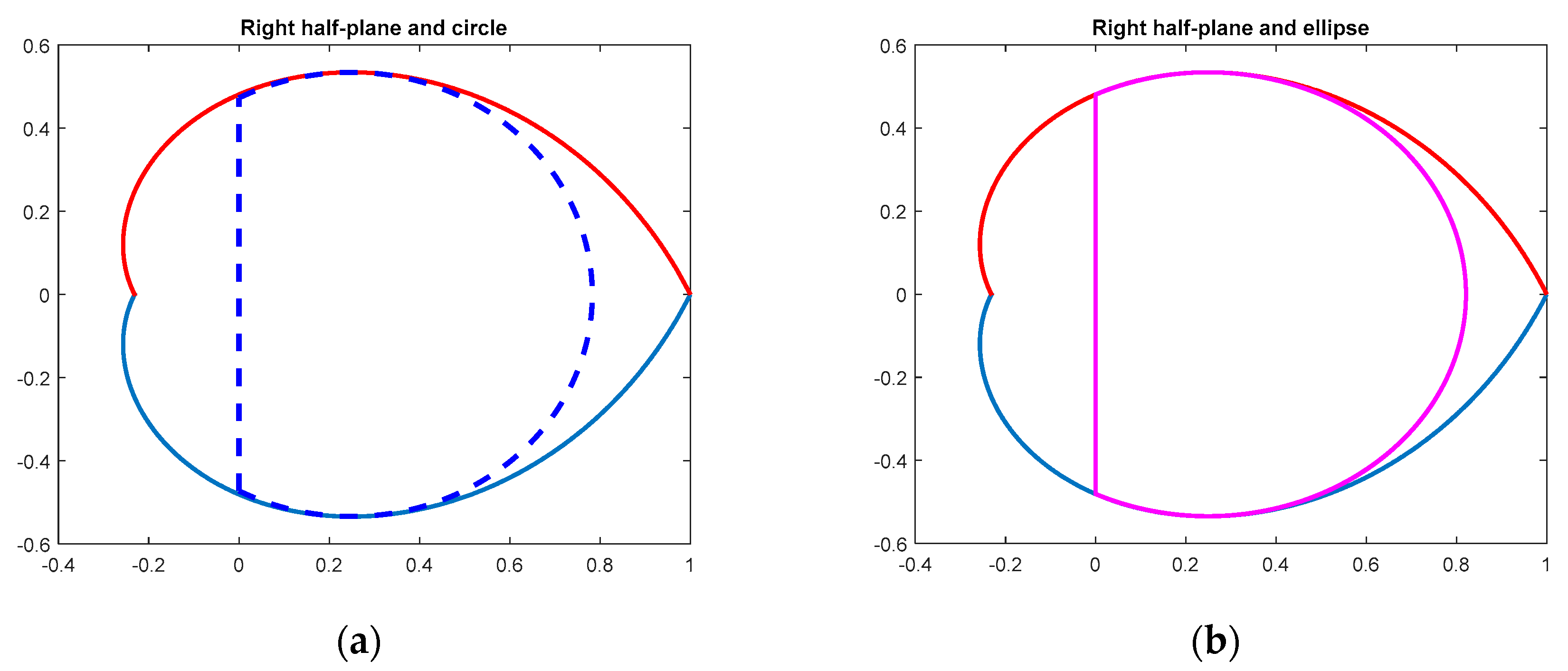
The next two options, c) and d), are appropriate for the case when poles with a nonnegative real part are required. Then it is advantageous to use the intersection of the right half plane with the inner circle or ellipse with bigger area than those in a) or b).
c) Right half-plane and circle
This option is suitable for angles bigger than 53°, when, for the extreme points given by Equations (14) and (15), it holds as follows: . The corresponding circle is centered in and its radius is set to . The resulting region is obtained as an intersection of the right half plane and the circle and the corresponding matrices are as follows:
- R11 = [0 0; 0 (xM^2 − r^2)];
- R12 = [−1 0; 0 − xM];
- R22 = [0 0; 0 1];
The approximation is depicted in Figure 8a.
d) Right half-plane and ellipse
The ellipse is centered in , as in the case of b), however, its x-semi-axis is increased, so that the ellipse reaches the intersection of the cardioid with the y-axis, denoted as y3. The resulting region is obtained as an intersection of the right half plane and the ellipse and the corresponding matrices, R11, R12, and R22, are calculated as follows:
- y3 = exp (−pi/(2*tan(fi*pi/180)));
- ak = xM*yM/sqrt (yM^2 − y3^2);
- bk = yM;
- R11 = [0 0 0; 0 − 1 − xM/ak; 0 −xM/ak −1];
- R12 = [−1 0 0; 0 0 (1/ak − 1/bk)/2; 0 (1/ak + 1/bk)/2 0];
- R22 = zeros (3, 3);
( is represented by fi in the program).
Though the last approximation (intersection of the right half plane and ellipse) gets closer to the right-hand side border than the inner ellipse (compare Figure 7b and Figure 8b), there is still a significant area not included in the approximation. All the above approximations basically avoid the domain close to point [1, 0]. The next novel combination of the shifted cone and ellipse is proposed to also include this area close to the border, since it can be important to make control feasible.
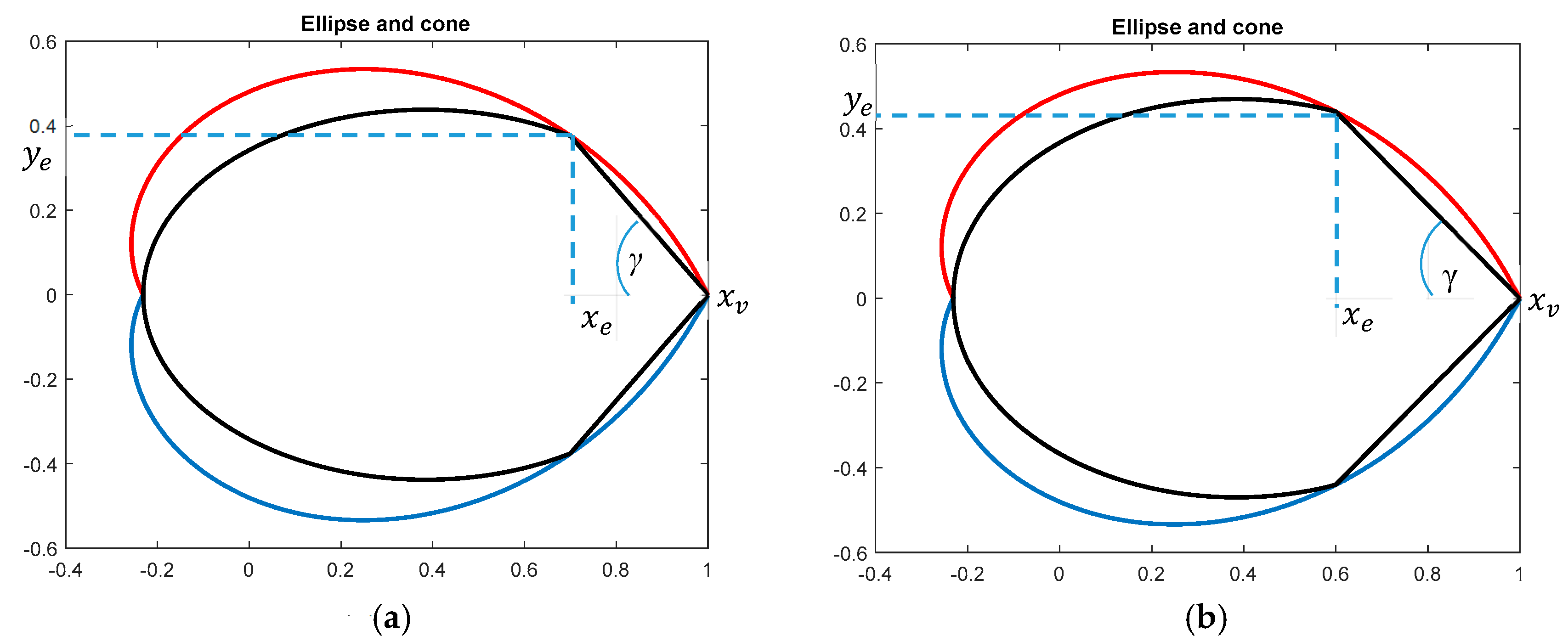
e) Ellipse-cone
This approximation considers the intersection of an angle with the vertex in [1, 0] and the elliptic region. The crossing point lies on the cardioid (logarithmic spiral) and is considered as a parameter to be chosen. In Figure 9, two variants for different choices of are shown.
The ellipse is centered in the middle of the cardioid x-axis, its x-semi-axis denoted as is maximized, and the y-semi-axis is derived so that it crosses , as follows:
- xse = (1 + x0)/2;
- ak = (1 − x0)/2;
- bk = ye*ak/sqrt (ak^2− (xe − xse)^2);
and the corresponding region matrices are as follows:
- R11e = [−1 – xse/ak; − xse/ak − 1];
- R12e = [0 (1/ak − 1/bk)/2; (1/ak + 1/bk)/2 0];
- R22e = zeros (2, 2).
The cone with the vertex in and inner angle corresponds to Figure 9 ( is represented by ga in the program). The respective region matrices for this shifted angle are as follows:
- ga = atan(ye/(1 − xe));
- R11v = [−xv*sin(ga)*2 0; 0 − xv*sin(ga)*2];
- R12v = [sin(ga) cos(ga); − cos(ga) sin(ga)];
- R22v = [0 0; 0 0].
The region matrices describing the intersection of the ellipse and angle can be obtained by taking and merging the above matrices for the ellipse and cone, as follows:
- Z = zeros (2, 2);R11 = [R11e Z; Z R11v];
- R12 = [R12e Z; Z R12v];
- R22 = [R22e Z; Z R22v].
Remark 2.
It should be noted that any regions can be combined, so that their intersection is considered, as in the latter case, where the intersection of the ellipse and angle is described by the resulting region matrices. regions can be also combined with other performance criterion. Often, pole placement is considered together with H2 or Hinf minimization.
Comparison of all the above approximations is illustrated on the example in the next section, providing the results for laboratory magnetic levitation plant.
4. Discrete-Time Robust Pole Placement Control for Magnetic Levitation (ML) Laboratory Plant
This section presents the results obtained for a robust state feedback pole placement controller designed for a laboratory magnetic levitation plant [20], for different choices of the region. The control aim in the ML system is to control the position of a magnetic ball levitating in the air-space. This position is controlled by the current in the coil (electromagnet) situated above the air-space. The ML can be modelled by a 3rd order nonlinear state space system. All state variables can be measured and used for control, as follows: Ball position, ball velocity, and current in the coil. All the details for ML state space nonlinear and linearized model can be found in [21]. The sampling period for a discretized model is 1ms. The robust state feedback pole placement controller was designed for the linearized uncertain model, Equation (1), obtained for 3 working points (WP) defined by 3 various ball positions corresponding to the state , as follows:
It is important to note that the ML system is unstable and the control variable (current in the upper coil) is limited, which also limits the required pole position.
The next choices of regions and the corresponding controllers were considered and compared as follows:
- Stabilization only: required pole region is unit circle;
- Elliptic inner approximation for 87° damping angle;
- New proposed ellipse-cone approximation for 50°, 60°, and 70° damping angles. For numerical reasons, in this case we considered and stability degree .
To track the ball position step changes, a PI controller was designed since the ML system itself does not include an integral term. The corresponding internal model principle for controller structure determination can be found, e.g., in Reference [22]. In all cases, the corresponding state feedback PI controller was designed and the corresponding closed loop poles were calculated.
The designed pole placement PI controller parameters for all the considered cases are summarized in Table 1. Note that the ellipse approximation yields about nine times bigger P gain and more than 20 times bigger I gain comparing to the new proposed ellipse-cone approximation. Furthermore, the ellipse-cone approximation provides a feasible solution to Equation (8), for a 50° damping angle, while the elliptic approximation provides feasible solution to Equation (8) only for damping angles bigger than 86°.
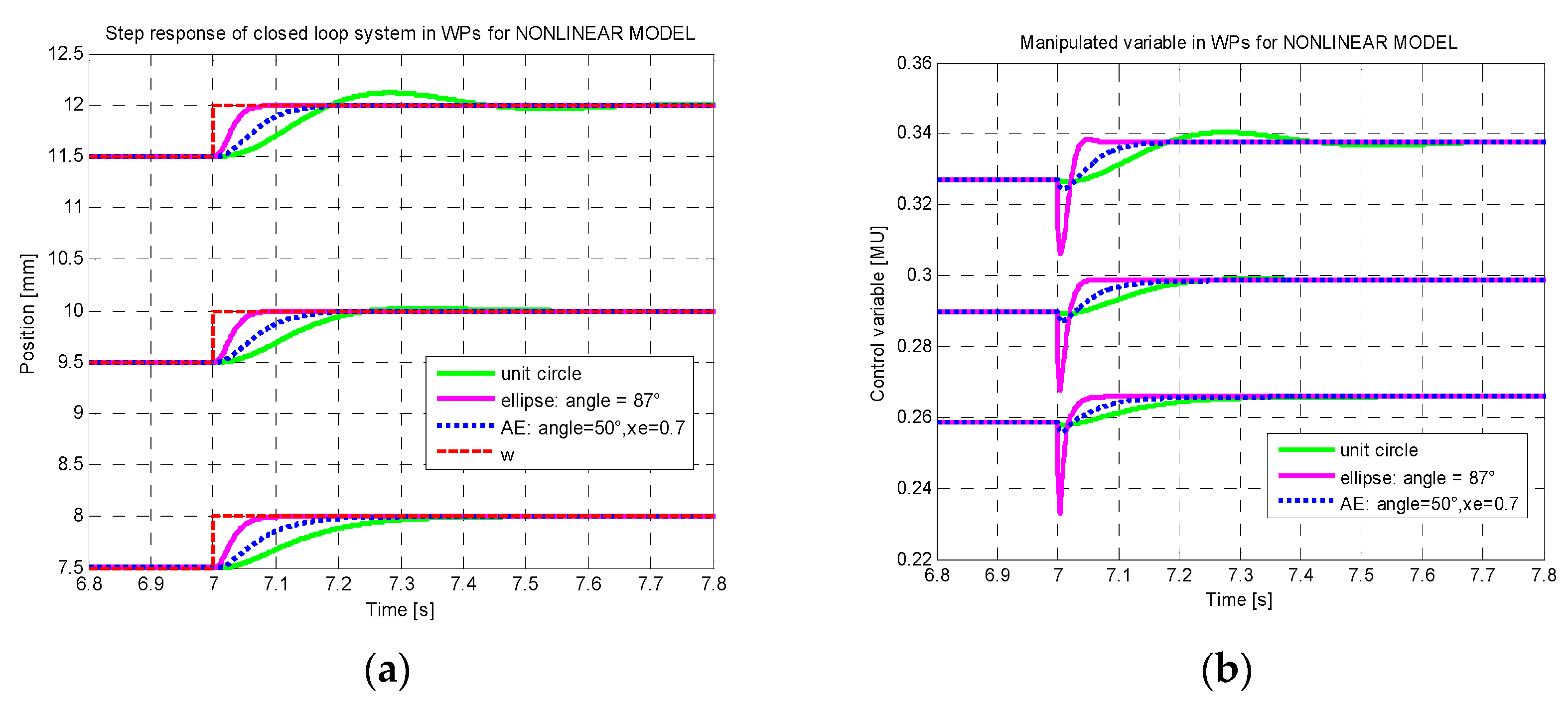
The designed controllers were then verified on a nonlinear simulation model. The obtained results are shown in Figure 10 and Figure 11. In Figure 10, the prescribed pole regions are depicted for all considered region variants, as well as for the corresponding closed loop poles. In all cases the poles are inside the prescribed region. Note that in the case of stabilization only (green), the poles are concentrated close to the stability border with almost no damping, which causes a response overshoot and a relatively longer settling time. The elliptic region, on the other hand, guarantees the damping. However, the poles are not allowed to keep closer to the point [1, 0], which indicates a too demanding control variable. The latter observation was approved by simulations for the nonlinear ML model. The results for 3 working points (3 different positions of levitating ball) are shown in Figure 11. Rapid significant changes of the control variable for elliptic approximation are outperformed by the ellipse-cone controller with both output and control variables smooth. This feature is important for the practical implementation of the designed controller.
For comparison we tried to design the continuous-time PI controller for the prescribed damping angle 60°—the corresponding convex cone region is shown in Figure 3a. Then we recalculated the continuous to the discrete-time PI controller (for the used sampling period 1ms). We verified the resulting controller on the nonlinear simulation model. We can conclude that, though the continuous-time controller design requires only 2 × 2 region matrices (the ellipse-cone approximation uses 4 × 4 region matrices), the recalculated continuous time PI controller provided significantly slower response than the originally designed discrete-time PI controller based on the ellipse-cone. Generally, the discrete-time controller recalculated from the continuous-time one provides a closed loop system performance that is not better (usually worse) than the continuous-time closed loop one [17].
5. Discussion and Conclusions
The paper provides the thorough study of discrete-time pole regions appropriate for a robust pole placement controller design. The main problem is finding adequate and computationally simple inner convex approximation for the nonconvex discrete-time system pole region corresponding to the prescribed damping. Previously published inner approximations for circle and ellipse are computationally simple, but they are too restrictive in cases where the realistic closed loop pole position close to the right-hand side pole region border stems from the real plant dynamics. The proposed ellipse-cone approximation much better approximates the original heart-shape region in the right-hand side part than the elliptic one (as shown in Figure 8 and Figure 9). This feature is important since the poles can be better tuned to receive the response, which is damped as required (contrary to the unit circle-based design). In comparison with elliptic approximation, the proposed ellipse-cone one provides wider possibilities to shape the response so that it is not too fast, which is important to obtain a less aggressive control action. This real plant feature is also inherent in the presented case study, a magnetic levitation laboratory system. Discrete-time pole placement results for magnetic levitation for various choices of the region are compared and illustrated in Figure 10. Though the discrete-time controller can be recalculated from the one designed in the continuous time domain, in general, the performance of the resulting closed loop system is usually worse than the continuous time original (in the best case, almost the same). This fact motivates the discrete-time controller design directly in the discrete-time domain.
The presented results provide the simple convex approximations to the originally nonconvex domain, with all the computational details. The authors believe this can contribute to solving the robust pole placement controller design problem for discrete-time systems with required resulting closed loop system damping (possibly combined with other performance requirements formulated by LMI) as simply as possible.
Author Contributions
Development of DR Region Mathematical Description, D.R.; Software, D.R. and M.H.; Validation, M.H., D.R.; Experiments, M.H.; Writing—Original Draft Preparation, D.R. and M.H.; Writing—Review and Editing, M.H. and D.R.
Funding
This research received no external funding.
Acknowledgments
The work has been supported by Slovak Scientific Grant Agency, grant No 1/0733/16.
Conflicts of Interest
The authors declare no conflict of interest. The funders had no role in the design of the study; in the collection, analyses, or interpretation of data; in the writing of the manuscript, or in the decision to publish the results.
References
- Boyd, S.; El Ghaoui, L.; Feron, E.; Balakrishnan, V. Linear Matrix Inequalities in System and Control Theory; SIAM: Philadelphia, PA, USA, 1994. [Google Scholar]
- Skelton, R.E.; Iwasaki, T.; Grigoriadis, K. A Unified Algebraic Approach to Linear Control Design; Taylor and Francis: London, UK, 1998. [Google Scholar]
- Ebihara, Y.; Peaucelle, D.; Arzelier, D. S-Variable Approach to LMI-Based Robust Control; Springer: London, UK, 2015. [Google Scholar]
- Liu, K.-Z.; Yao, Y. Robust Control: Theory and Applications; John Wiley & Sons (Asia): Singapore, 2016. [Google Scholar]
- Mansouria, B.; Manamannia, N.; Guelton, K.; Djemai, M. Robust pole placement controller design in LMI region for uncertain and disturbed switched systems. Nonlinear Anal. Hybrid Syst. 2008, 2, 1136–1143. [Google Scholar] [CrossRef] [Green Version]
- Dos Santos, J.F.S.; Pellanda, P.C.; Simões, A.M. Robust pole placement under structural constraints. Syst. Control Lett. 2018, 116, 8–14. [Google Scholar] [CrossRef]
- Peaucelle, D.; Arzelier, D.; Bachelier, O.; Bernussou, J. A new robust D-stability condition for real convex polytopic uncertainty. Syst. Control Lett. 2000, 40, 21–30. [Google Scholar] [CrossRef]
- Botto, M.A.; Babuška, R.; da Costa, J. Discrete-time robust pole-placement design through global optimization. In Proceedings of the 15th IFAC World Congress, Barcelona, Spain, 21–26 July 2002. [Google Scholar]
- Chilali, M.; Gahinet, P.; Apkarian, P. Robust pole placement in LMI regions. IEEE Trans. Autom. Control 1999, 44, 2257–2270. [Google Scholar] [CrossRef] [Green Version]
- Boroujeni, E.A.; Daryabor, A.; Momeni, H.R. Designing robust pole placement control for Roll Motions of Ships via LMIs. In Proceedings of the IEEE International Conference on Control, Automation and Systems, Seoul, Korea, 14–17 October 2008. [Google Scholar]
- Aunsiri, T.; Numanoy, N.; Hemsuwan, W.; Srisertpol, J. Servo System Using Pole-Placement with State Observer for Magnetic Levitation System. Lect. Notes Electr. Eng. 2014, 309, 921–926. [Google Scholar]
- Rao, P.S.; Sen, I. Robust pole placement stabilizer design using linear matrix inequalities. IEEE Trans. Power Syst. 2000, 15, 313–319. [Google Scholar] [CrossRef]
- Turner, R.; Walton, S.; Duke, R. Robust High-Performance Inverter Control Using Discrete Direct-Design Pole Placement. IEEE Trans. Ind. Electron. 2011, 58, 348–357. [Google Scholar] [CrossRef]
- Lassere, J.B. An Introduction to Polynomial and Semi-Algebraic Optimization; Cambridge University Press: Cambridge, UK, 2015. [Google Scholar]
- Rosinová, D.; Holič, I. LMI Approximation of Pole-region for Discrete-time Linear Dynamic Systems. In Proceedings of the 15th International Carpathian Control Conference, Velké Karlovice, Czech Republic, 28–30 May 2014; pp. 497–502. [Google Scholar]
- Rosinová, D.; Hypiusová, M. Robust Pole Placement DR—regions for Discrete-time Systems. In Proceedings of the 22nd International Conference on Process Control, Štrbské Pleso, Slovakia, 11–14 June 2019. [Google Scholar]
- Isermann, R. Digital Control Systems; Springer: Berlin/Heidelberg, Germany, 1981. [Google Scholar]
- Morari, M.; Zafiriou, E. Robust Process Control; Prentice Hall: Upper Saddle River, NJ, USA, 1989. [Google Scholar]
- Lofberg, J. YALMIP: A toolbox for modelling and optimization in Matlab. In Proceedings of the CACSD Conference, Taipei, Taiwan, 2–4 September 2004. [Google Scholar]
- Magnetic Levitation System 2EM—User’s Manual; Inteco Ltd.: Krakow, Poland, 2008.
- Balko, P.; Rosinová, D. Modeling of magnetic levitation system. In Proceedings of the 21st International Conference on Process Control, Štrbské Pleso, Slovakia, 6–9 June 2017. [Google Scholar]
- Francis, B.A.; Wonham, W.M. The internal model principle of control theory. Automatica 1976, 12, 457–465. [Google Scholar] [CrossRef]
Figure 1.
Stable system pole regions. (a) Continuous-time system: Open left half plain of the convex plane; (b) discrete-time systems: Interior of the unit circle.
Figure 1.
Stable system pole regions. (a) Continuous-time system: Open left half plain of the convex plane; (b) discrete-time systems: Interior of the unit circle.

Figure 2.
Pole regions for the prescribed stability degree (corresponding to the system exponential decay rate). (a) Continuous-time system: Shifted left half plain of the convex plane; (b) discrete-time systems: Interior of the “shrinked” unit circle – circle centered in [0, 0] with radius 1/sqrt(α), where α > 1.

Figure 3.
Pole regions for the prescribed relative damping (corresponding to a ratio of the imaginary and real part of the pole). (a) Continuous-time system: Interior of the convex cone with vertex angle corresponding to the damping); (b) discrete-time systems: The space between two symmetric logarithmic spirals.

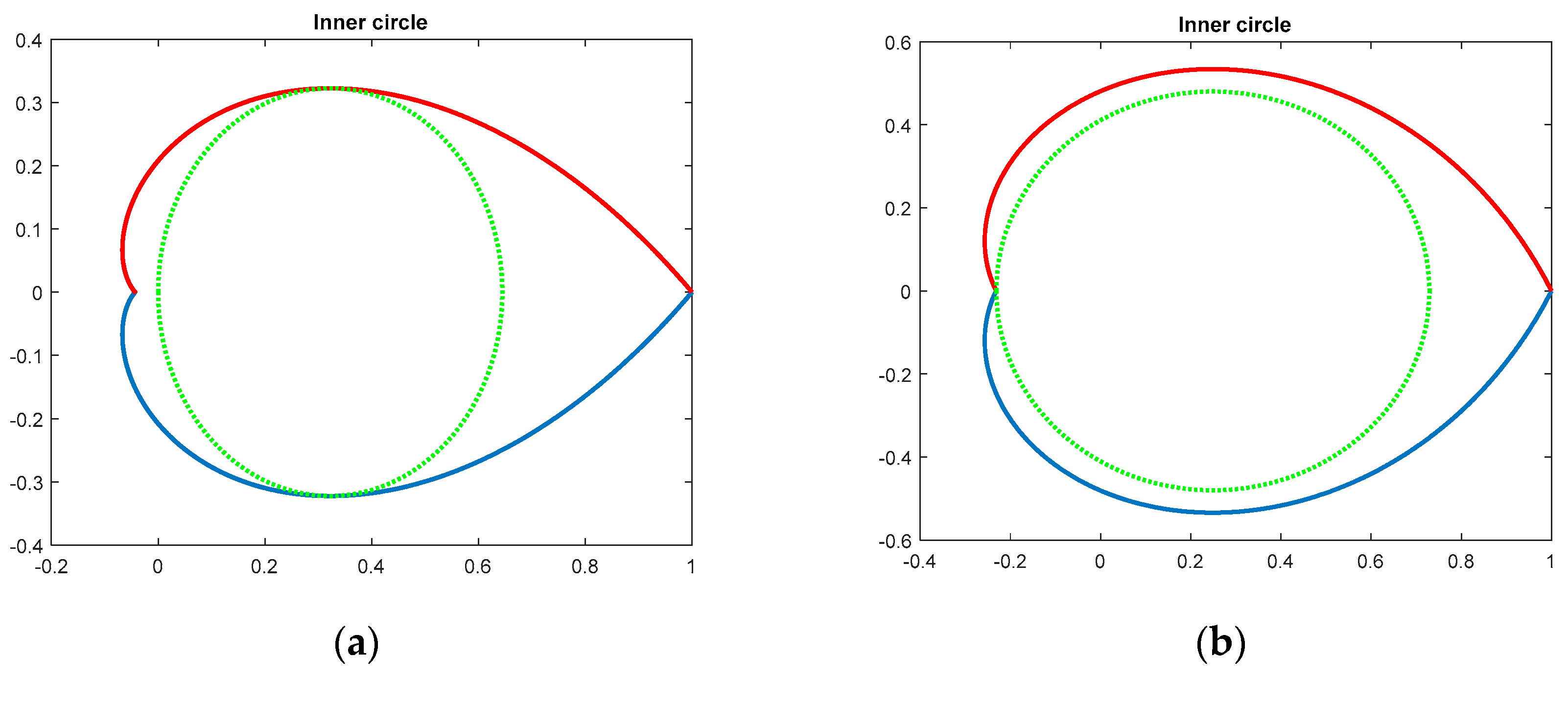
Figure 4.
Inner circle (green) and elliptic (black) approximations to the cardioid region.

Figure 5.
Extreme points of a logarithmic spiral, Equation (13): Upper point, , intersection with negative real axis
Figure 5.
Extreme points of a logarithmic spiral, Equation (13): Upper point, , intersection with negative real axis

Figure 6.
Inner circle approximation of cardioid: (a) For a 45° damping angle and (b) for a 65° damping angle.
Figure 6.
Inner circle approximation of cardioid: (a) For a 45° damping angle and (b) for a 65° damping angle.

Figure 7.
Inner elliptic approximation of cardioid: (a) For a 45° damping angle and (b) for a 65° damping angle.
Figure 7.
Inner elliptic approximation of cardioid: (a) For a 45° damping angle and (b) for a 65° damping angle.

Figure 8.
Approximation given by the intersection of the right half plane with circle (a) and ellipse (b) (65° damping angle).
Figure 8.
Approximation given by the intersection of the right half plane with circle (a) and ellipse (b) (65° damping angle).

Figure 9.
Approximation given by the intersection of the angle and ellipse (a) for and (b) for .

Figure 10.
Prescribed pole regions and corresponding closed loop poles for tested variants: (a) The overall regions and (b) the detail on pole location near the right-hand side border of regions.
Figure 10.
Prescribed pole regions and corresponding closed loop poles for tested variants: (a) The overall regions and (b) the detail on pole location near the right-hand side border of regions.

Figure 11.
Simulation results for the nonlinear ML model in 3 working points (WP) for the designed robust pole placement controller for unit circle (green), elliptic approximation for damping angle 87° (magenta), and ellipse-cone (AE: blue dots): (a) Output variable—ball position; (b) control variable—current in the coil.


Table 1.
State feedback PI controller parameters designed using Equation (8) for the considered regions.
Table 1.
State feedback PI controller parameters designed using Equation (8) for the considered regions.
| D_R Region | P | I |
|---|---|---|
| Unit circle | [106.7, 2.47, −0.617] | 0.3527 |
| Ellipse (87°) | [952.4, 9.75, −0.653] | 26.88 |
| Ellipse-cone (70°) | [134.2, 2.55, −0.275] | 1.222 |
| Ellipse-cone (60°) | [154.7, 2.93, −0.317] | 1.420 |
| Ellipse-cone (50°) | [190.7, 3.56, −0.368] | 1.831 |
© 2019 by the authors. Licensee MDPI, Basel, Switzerland. This article is an open access article distributed under the terms and conditions of the Creative Commons Attribution (CC BY) license (http://creativecommons.org/licenses/by/4.0/).
Share and Cite
MDPI and ACS Style
Rosinová, D.; Hypiusová, M. LMI Pole Regions for a Robust Discrete-Time Pole Placement Controller Design. Algorithms 2019, 12, 167. https://0-doi-org.brum.beds.ac.uk/10.3390/a12080167
AMA Style
Rosinová D, Hypiusová M. LMI Pole Regions for a Robust Discrete-Time Pole Placement Controller Design. Algorithms. 2019; 12(8):167. https://0-doi-org.brum.beds.ac.uk/10.3390/a12080167
Chicago/Turabian StyleRosinová, Danica, and Mária Hypiusová. 2019. "LMI Pole Regions for a Robust Discrete-Time Pole Placement Controller Design" Algorithms 12, no. 8: 167. https://0-doi-org.brum.beds.ac.uk/10.3390/a12080167
Note that from the first issue of 2016, this journal uses article numbers instead of page numbers. See further details here.