Long Short-Term Memory Neural Network Applied to Train Dynamic Model and Speed Prediction

1
School of Electronic and Information Engineering, Beijing Jiaotong University, Beijing 100044, China
2
National Engineering Laboratory for Urban Rail Transit Communication and Operation Control, Beijing 100044, China
3
Traffic Control Technology Co., Ltd., Beijing 100070, China
*
Author to whom correspondence should be addressed.
Algorithms 2019, 12(8), 173; https://0-doi-org.brum.beds.ac.uk/10.3390/a12080173
Submission received: 26 July 2019
/
Revised: 8 August 2019
/
Accepted: 14 August 2019
/
Published: 16 August 2019
Abstract
:The automatic train operation system is a significant component of the intelligent railway transportation. As a fundamental problem, the construction of the train dynamic model has been extensively researched using parametric approaches. The parametric based models may have poor performances due to unrealistic assumptions and changeable environments. In this paper, a long short-term memory network is carefully developed to build the train dynamic model in a nonparametric way. By optimizing the hyperparameters of the proposed model, more accurate outputs can be obtained with the same inputs of the parametric approaches. The proposed model was compared with two parametric methods using actual data. Experimental results suggest that the model performance is better than those of traditional models due to the strong learning ability. By exploring a detailed feature engineering process, the proposed long short-term memory network based algorithm was extended to predict train speed for multiple steps ahead.
1. Introduction
Railway transportation, an effective means to increase the efficiency of energy consumption and relieve the traffic congestion problem, has been stressed as an ideal transport mode in large cities [1]. To achieve safe and efficient operation, train control algorithms remain a key technical issue in the process of the development of railway systems [2]. Traditionally, with the help of signal devices, the train operation is accomplished by skilled drivers. However, this human-based train operation method lacks precise consideration, which may lead to a poor performance of energy consumption, service quality and safety [3]. Recently, with the combination of communication and computer technologies, the automatic train operation has become a research hotspot [4,5,6], which also has been used in many newly-built railway systems.
Different from the manual labor based method, an automatic train operation system can provide a better operation performance by optimizing train control decisions. Many indicators that describe the running state of the train such as punctuality, riding comfort and energy efficiency can be remarkably improved by automatically adjusting the commands of train accelerating, coasting and braking process. The automatic train operation system mainly solves three arduous tasks: train dynamic model construction [7], speed profile optimization [8] and train speed control [9].
Establishing train dynamic model is regarded as a fundamental and significant problem among these tasks, since all the subsequent studies such as speed profile optimization and train speed control are built on it. Many methods have been proposed to obtain a precise dynamic model [10,11,12,13]. These methods that build upon the Davis formula can be classified into two categories, i.e., single-point train control models and multi-point train control models [10]. In the first one, which has been investigated for many years, the train, consisting of a locomotive and many carriages, is treated as a single-mass model. Although the inner characteristics produced by the coupled system cannot be accurately expressed, this type of model has the advantages of deployment feasibility and calculation simplicity [11]. In the second class, a more complicated model is rigorously designed, which takes the impacts of adjacent carriages into consideration [12]. All of these methods belong to the parametric approaches, where the structure of the model is determined under certain theoretical assumptions and the values of parameters are calculated based on analytical equations, such as Newton’s law and the Davis formula. Nevertheless, a precise train dynamic model is hard to acquire due to unrealistic assumptions and changeable environments [13]. How to obtain an appropriate dynamic model that can reflect the actual condition of train operation remains a crucial task.
To find an innovative way to deal with the above-mentioned task, different from the parametric approaches, we propose to apply deep learning algorithms to solve the problem of train dynamic model construction. This kind of data-driven method has been widely investigated in highway trajectory prediction and traffic speed prediction to replace the traditional parametric approach [14,15,16]. Data-driven methods also have been introduced for train trajectory tracking [17], train station parking [18] and train operation modeling [19]. Inspired by these studies, in this paper, a long short-term memory (LSTM) neural network is carefully developed to build the train dynamic model in a nonparametric way. LSTM networks [20] are called advanced recurrent neural networks with additional features, which can keep a memory of previous inputs, resulting in a good performance of handling time series problems such as the train dynamic model and the speed prediction. Using the same algorithm inputs as traditional parametric approaches (analog output, traction brake, rail slope and train speed), we explore a detailed feature engineering process, where lagged features of the actual data can be captured. By deliberately tuning the parameters of the proposed LSTM based model, more accurate outputs can be obtained. We compared the proposed approach with two other algorithms: (i) a parametric approach in which the parameters are optimized using the fruit fly optimization algorithm; and (ii) a traditional train dynamic model that is currently being used in real train control systems. The proposed model was validated against the actual data from Shenzhen Metro Line No. 7 in China and Beijing Yanfang Metro Line in China. Experimental results demonstrate that the output accuracy was remarkably enhanced compared to these algorithms. Furthermore, by combining lagged features and statistical features, we captured the long-term pattern of the data and extended the proposed LSTM based algorithm to predict train speed for a longer period of time.
2. Related Work
As mentioned above, parametric approaches of the train dynamic model can be divided into two classes. For the first class, Howlett [21] pioneered a single-mass model, where the train is controlled using a finite sequence of traction phases and a final brake phase. The Lagrangian multiplier method is applied to search fuel-efficient driving solutions in this work. To minimize energy consumption, in [22], the authors presented an analytical solution to obtain the sequence of optimal controls. In this calculation algorithm, the in-train force is ignored. With the purpose of shortening the computation time, Wang et al. [23] formulated the single-mass dynamic model as a mixed-integer linear programming (MILP) problem. By approximating and relaxing the high-order nonlinear terms, the global optimal solution can be found in polynomial time. Single-point train control models have also been studied [24,25]. For the second category, to describe the internal relationship among the adjacent cars, Gruber et al. [26] first put forward a multi-point train control model, where a switching policy and linear suboptimal controllers are designed to model this large-scale system. In [27], a multi-point based longitudinal train model was proposed, where the model parameters are tuned according to the experimental environment. This model was validated against actual data from Spoornet. In [28], the authors established a cascade-mass-point model to simplify the multi-point model. Taking simplicity, cost-effectiveness and implementation convenience into consideration, the issue of output regulation with measurement feedbacks is well solved in this model. Besides, many researchers pay attention to building an appropriate multi-point dynamic model in high-speed railways [10,29,30].
It is worth mentioning that some data-driven algorithms have been introduced in the area of train operation systems. The work in [18,31,32,33] attempted to solve the train automatic stop control problem using machine learning methods. Specifically, Chen et al. [33] employed a regression neural network to estimate the train station parking error. The algorithm parameters are deliberately adjusted to reduce parking errors. In [32], the authors proposed adopting regression algorithms to analyze the train stopping accuracy. By extracting relevant features through feature engineering, the ridge regression and the elastic net regression are employed to build models to reflect the relationship between the features and the stopping accuracy. These studies only consider the train stop control problem that occurs when the train stops at stations. In [17], coordinated iterative learning control schemes were designed for train trajectory tracking. This method can learn to improve control performances from previous executions, which requires less system model knowledge. The speed tracking errors are reduced via repeated operations of the train. Three data-driven train operation models were proposed in [19]. By summarizing an expert system from the domain driving experience, K-nearest neighbor, Bagging-CART and Adaboost are employed for train operation. Then, these models are improved via a heuristic train parking algorithm to ensure the parking accuracy. Compared to the methods in [32,33], the whole operation process is analyzed in this paper. Reinforcement learning based algorithms were employed to solve optimal control problems in [34]. An adaptive actor-critic learning framework is carefully designed with the virtual reference feedback tuning. This approach was validated to learn nonlinear state-feedback control for linear output reference model tracking, which is innovative and can be applied to the train control system. Besides, data-driven methods also have been used for fault detection and diagnosis in the area of rail transit [35]. These inspiring studies give us a new angle to view the problem of building the train dynamic model.
Data-driven algorithms have been widely used in intelligent transportation systems [16,36,37]. In the area of traffic forecasting and trajectory prediction, data-driven approaches tend to outperform the parametric approaches. In [38], a fuzzy neural network is employed to increase the prediction accuracy of the traffic flow. The support vector machine [39] also has been introduced for trajectory prediction. The machine learning algorithms have the advantage of dealing with high dimensional and nonlinear relationships, which is especially suitable for establishing train dynamic model and train speed prediction on account of the dynamic and nonlinear nature [40]. Among the machine learning algorithms, the recurrent neural network (such as the LSTM network) is designed to seize the features of the temporal and spatial evolution process. Several studies [41,42,43] focused on the use of LSTM neural networks for traffic forecasting and demonstrated the advantages of this kind of algorithm. Encouraged by the successful applications of LSTM based algorithms in the domain of transportation, we propose to employ LSTM networks for train dynamic model construction and train speed prediction, since the train operation process can be regarded as a time sequence problem.
3. Methodology
3.1. Parametric Based Train Dynamic Model
To facilitate understanding, in this subsection, we briefly introduce a classical single-point train dynamic model. Other types of dynamic models (such as multi-point models) can be considered as optimized or expanded versions of this model. By ignoring the in-train force and assuming continuous control rates, the model can be formulated as [44]
where x, v and t denote the train displacement, velocity and time, respectively. represents the total mass of the train, where is the mass of the ith carriage. is the train traction force while denotes the train braking force. and represent the relative accelerating and braking coefficients, respectively. Given a certain train position x, describes the impacts of the gradient resistances and curve resistances. is the Davis formula, which expresses the relationship between the train speed and the aerodynamic drag, where , and indicate the resistance parameters.
In this model, let denote the set of train positions in a certain operation area. The location data can be obtained by locating devices, i.e., balises, which are extensively deployed in the European Train Control System and the Chinese Train Control System [45]. With low time delay, a balise transmits the position data to the passing train. The velocity of the train can be similarly captured by track-side and on-board devices. Given the fixed parameters of the dynamic model (, , , , and ), the inputs and the outputs of the model are shown in Figure 1. As can be seen in Figure 1, when a certain train passes , the inputs of the dynamic model are , , and . Using Equations (1) and (2), the model output can be calculated.
Since some of the model parameters are difficult to acquire in real-world scenarios, their values are arbitrarily assigned, resulting in a poor performance of this parametric approach. Furthermore, the velocity of the train varies in a wide range during the operation process. By adjusting the control commands, the operation process can be divided into four phases: train acceleration, train coasting, train cruising and train braking. At different operation phases, the parameters and disturbance factors have different influences of the model outputs. Thus, Equations (1) and (2) may change into various complicated multivariate nonlinear functions, which increases the difficulty of system modeling.
3.2. LSTM Based Train Dynamic Model: Problem Statement
To overcome the aforementioned disadvantages of the parametric approach, we propose a data-driven approach to address the issue of train dynamic model construction, where the LSTM network is applied. Besides, by deliberately designing the lagged features and statistical features, we extend the proposed LSTM based algorithm to predict train speed for multi-step ahead. To be more specific, the train dynamic model can be considered as an approach to get the train speed of the next time step. Since LSTM networks have the capacity to model long-term dependencies, our proposed model can obtain the train speeds for next n time steps.
For clarity, in this subsection, we review the problem of the train dynamic model. Note that the model inputs are exactly the same as the aforementioned parametric approach. Formally, let and denote the sets of observable features and target outputs, respectively. Similar to Section 3.1, all features (model inputs) can be instantly seized at any time step. represents the set of previous time steps, which can be written as . For and , we express the feature vector as the values of features seized at th previous time step, where n denotes the number of features. The feature matrix can be formulated as
where means the jth feature captured at ith time step.
In addition, we denote . For and , is defined as the value of model output at qth time step in the future. is defined as the output vector. Using a deep learning method, a regression function h is trained, which can be written as
where represents the set of algorithm parameters.
With the purpose of reducing the gap between the predicted outputs and the actual values, the loss function should be minimized
where l represents the number of samples. denotes the vector of actual values. In our scenario, according to Figure 1, using feature matrix generated by , , and , the proposed approach is capable of getting the predicted train speeds .
3.3. LSTM Network Structure
The LSTM network is a variant of deep neural networks, which was first introduced by Hochreiter [20]. Distinguished from traditional neural networks, there exists an internal hidden state in the units that constitutes the LSTM network. Generally, an LSTM network is made up of one input layer, one recurrent hidden layer and one output layer. The unit in the recurrent hidden layer is termed as the memory block, which consists of memory cells and adaptive, multiplicative gating units. In the memory cell, the state vector is saved to aggregate the previous input data. By tuning the parameters of gating units, the input data, the output data and the state data are mixed to update the current state. The control mechanism is summarized as follows. Note that all the symbol definitions can be found in Table 1.
Without ambiguity, at each time iteration t, let denote the hidden layer input feature which is directly fed to the LSTM cell through the input gate. The input gate can be written as [46]
Assuming the dimensions of and are and , respectively, the dimension of is . is defined as the dimension of the state vector. , and are decided to control the effects of the layer input and the layer output of previous time step on the output of input gate .
To deal with the gradient diffusion and the gradient explosion problems [47], in LSTM networks, the forget gate is deliberately designed
According to Equation (8), once the contents of the LSTM cell are out of date, the forget gate helps to update parameters by resetting the memory block. Similarly, the dimension of is .
The output gate is defined as
The definitions of , , and are listed in Table 1.
To update the cell statement, is defined as the state update vector ,which is calculated as
In Equation (10), represents the hyperbolic tangent function. The reason for using this particular function is that other activation functions (e.g., the rectified linear unit) may have very large outputs and cause the gradient explosion problem [48]. The hyperbolic tangent function can be written as
Based on the results of Equations (7) and (11), at a certain time step t, the current cell state is updated by
where ∘ represents the scalar product of two vectors. By observing Equation (12), thanks to the control of the input gate and the forget gate, one can find that the current input and long-term memories are combined to form a new cell state.
At last, the hidden layer output is decided by the output of the output gate and the current cell state
The internal structure of an LSTM cell is shown in Figure 2.
The training process can be regarded as a supervised learning process and many objective functions are designed to minimize the average differences between the outputs of the LSTM network and the actual values. In the training process, the parameters (such as the weight matrices and the biases vectors) are optimized. Errors are intercepted at the LSTM cells and are vanished thanks to the forget gate. The gradient descent optimization algorithm is adopted to obtain the gradient of the objective function, and then the Back Propagation Through Time (BPTT) [49] algorithm is used to train and update all the parameters to increase the prediction accuracy. The derivations of the training process are not covered in this paper due to space restrictions. One can refer to the work in [46] for detailed execution steps.
Through multiple iterations, ideally, the parameters will gradually converge to the global optimum while the training process is finished. However, due to the substantial number of hyperparameters and the deep network structure, the gradient descent algorithm may be trapped to the local optimum, resulting in the degradation of output accuracy and the prolongation of training time. To cope with this problem, in this paper, the Adaptive Moment estimation (Adam) optimization algorithm [50] is employed to avoid low efficiency and local optimum.
Note that, even though only one hidden layer exits in the network, the LSTM network is considered as a deep learning algorithm due to the recurrent nature. Similar to convolutional neural networks, more hidden layers can be stacked to seize high-dimensional characteristics. However, previous studies show that adding hidden layers may not significantly improve the algorithm performance over a single layer [51,52]. Thus, in this paper, the aforementioned standard LSTM network structure is adopted where one hidden layer is deployed to save storage and computing resource.
3.4. Algorithm Implementation
3.4.1. Data Preparation
In this study, to prove the practicality of the proposed LSTM network based algorithm, we used actual runtime data as the network inputs. The actual in-field data were gathered by the Vehicle On Board Controller (VOBC) from Shenzhen Metro Line No. 7 in China and Beijing Yanfang Metro Line in China. The dataset of Shenzhen Metro Line consists of three subsets, which separately record the train operation data of a certain train on three days, i.e., 7 April 2018, 8 April 2018 and 11 July 2018. The dataset of Beijing Yanfang Metro Line includes the operation data collected on 13 May 2019. For example, the subset on 7 April 2018 contains 381,637 records which describe the driving process through the whole day. The relevant information of one record is listed in Table 2.
As can be seen in Table 2, the information of the train operation state was meticulously recorded. The vast amounts of data offer the advantageous support to apply data-driven algorithms. To keep consistent with the inputs of the traditional dynamic model presented in Section 3.1, we chose four raw features as the inputs of the proposed algorithm: analog output, traction brake, train speed and slope. These four features for a certain operation process are shown in Figure 3.
- Analog output: Analog output is a continuous variable, which is outputted by electric motors. This feature is used to control the train to accelerate or decelerate. It reflects the absolute value of the train braking force and the train traction force .
- Traction brake: Traction brake is a categorical variable, which implies the direction of analog output and gives the signs of and .
- Train speed: At each time iteration t, the train speed is accurately recorded by VOBC.
- Slope: Slope represents the track gradient which impacts the gradient resistances.
One can find that extra information is not added to our algorithm compared to the traditional method. The purpose is to prove that the performance improvement of the proposed approach depends on the algorithm itself rather than the extension of inputs.
3.4.2. Data Preprocessing
In reality, operation data are collected by many on-board sensors and trackside equipments. Considering the practical working environment, the sensors and actuators may fail to generate data due to line fault, equipment failure, communication quality, etc. This situation further leads to the problem of missing values. Missing values of the dataset reduce the fitting effect and increase the model bias, resulting in a poor performance of regression and prediction. For LSTM based algorithms, the effect of missing values is more serious. LSTM networks fail to run since null values cannot be calculated during the error propagation process. The missing values can be arbitrarily set to zero or other statistical values (such as the most frequent non-missing value). However, this treatment causes a great disturbance when handling time series problems. In this paper, similar to Cui [43], a masking mechanism is proposed to solve the problem of missing values.
In the masking mechanism, we predefine a mask value and the missing values are directly set as . At each iteration t, if one of the raw features is invalid, all the raw features, i.e., , , and , are set to . In this paper, the mask value is assigned as null. For a feature matrix , if there exists a missing element in , the element equals and the training process at the kth step will be skipped. Thus, the state vector is directly fed to the ()th time step. Note that the issue of continuous missing values can also be solved using this masking mechanism.
3.4.3. Feature Engineering
Feature engineering is a vital part of data analysis. The quality of results of deep learning algorithms heavily relies on the quality of the input features. For the traditional train dynamic model, as can be seen in Figure 1, with the inputs of , and , the current speed can be calculated. To be consistent with the previous model, in the proposed dynamic model, the raw features, i.e., , , and , are directly fed into the LSTM cells after removing the missing values. To facilitate understanding, in this paper, we do not use abbreviations for these features.
Considering the problem of train speed prediction, since we expect to obtain the train speeds for next n time steps, more delicate descriptions of the features should be made to capture more information from previous data. For this reason, we establish a different set of features as inputs for train speed prediction. The set contains three types of features, i.e., lagged features, crossed features and statistical features. All features are produced by , , and slope, which are listed above.
The lagged features imply the instantaneous values of the previous time steps, which are defined as:
- At time iteration t, the train speed of kth step earlier: , where .
- At time iteration t, the analog output of kth step earlier: , where .
The statistical features capture the changes of the input values in the previous period:
- The average value of train speed of past k steps: , where .
- The standard deviation of train speed of past k steps: , where .
- The difference of train speed between the previous kth step and the current step: , where .
- The average value of analog output of past k steps: , where .
- The standard deviation of analog output of past k steps: , where .
- The difference of analog output between the previous kth step and the current step: , where .
Since recent data play a more important role for a time series problem, the crossed features are designed as:
- The product of train speed of past k steps: , where . For example, .
In total, 43 features are extracted for the train speed prediction task.
3.4.4. Offline Training and Online Predicting
When the feature engineering process is done, the features are fed to the input layer. To eliminate the effect of index dimension and quantity of data, all features are normalized using the Min-Max Normalization method shown in Equation (14).
where and represent the minimum and maximum of a certain feature, respectively.
Each neuron in the input layer is connected to each LSTM cell in the hidden layer. Note that its number should match the dimension of the input data. In this paper, the activation functions of the input gate, the output gate and the forget gate are selected as the standard logistics sigmoid function shown in Equation (15)
In the recurrent hidden layer, as described in Section 3.3, the “meaningful parts” are abstracted from the input time series. The parameters are updated using the Adam optimization algorithm and the BPTT algorithm. These “higher-level features” are then combined in the output layer. The output layer is also termed as the dense layer to produce the predicted train speeds of future time steps. As a regression problem, the output layer has only one neuron. In this paper, the optimization of the dense layer can be considered as a linear regression problem, i.e., the activation function of the output layer is set as a linear function. The loss function in this paper adopts the Mean Absolute Error (MAE) loss
The offline training phase ends when the error of the algorithm outputs meets the preset threshold. The set of parameters (such as the weight matrices and the biases vectors) can be obtained, which approximately describes the regression function in Equation (5).
In the online predicting phase, the actual data gathered by VOBC are fed to the trained LSTM network. After extracting the raw features, the proposed data-driven algorithm can output the prediction of the next time step, whose functionality can serve as the train dynamic model. In addition, with the feature engineering process, the train speeds for next n time steps can be obtained.
4. Experiment
We conducted comprehensive experiments to verify the effectiveness of the proposed algorithm. The data from Shenzhen Metro Line No. 7 in China constitute the training set and the validation set while the data from Beijing Yanfang Metro Line in China form the test set. The number of samples of Shenzhen Metro Line is 644,272 and the time series split method in Scikit-learn was employed to split the training set and the validation set. Different from the classical cross-validation techniques such as k-fold and shuffle split, time series split can prevent the data leakage problem. The core idea of this method is to return first k folds as the training set and the ()th fold as the validation set. One may refer to Swami [53] for more information. The number of samples of Yanfang Metro Line is 71,638. The sample interval of VOBC is 200 ms. For example, the time length of the samples of Yanfang Metro Line is h. The proposed algorithm was trained using the Keras framework. The training process was accelerated by the CUDA acceleration technology. The standard LSTM network structure with one hidden layer was adopted unless otherwise stated. The mini-batch gradient descent method and the BPTT algorithm were used during the parameter update process. For the Adam optimization algorithm, the hyperparameters , and were set to , and , respectively. Besides, the early stopping mechanism was used to limit the overfitting problem. In Section 4.1 and Section 4.2, the experimental results of the proposed train dynamic model and the n steps speed prediction are provided, respectively.
4.1. The Proposed Train Dynamic Model
We first studied the impact of hyperparameters on the algorithm performance. After the parameter adjustment, the proposed model was validated against the data of Beijing Yanfang Metro Line. With the intention of demonstrating that the proposed algorithm has a superior performance, we compared the proposed algorithm with parametric-based train dynamic models. To measure the effectiveness of different algorithms and analyze the influence of hyperparameters, in addition to the MAE, the Mean Squared Error (MSE) and the R-Square (R2) were calculated.
The MSE is defined as:
The R2 is defined as:
where denotes the mean of the actual value.
4.1.1. Influence of Hyperparameters
The raw features (analog output, traction brake, train speed and slope) were extracted from the training data and the missing values were removed using the masking mechanism. After the feature engineering process, the designed features were fed to the LSTM network sequentially. The hyperparameters have a great influence on the output accuracy and should be carefully tuned. The influences of the hidden size, the batch size, the learning rate and the number of hidden layers were studied (see Section 4.1.1). The hyperparameter with the best performance is marked in bold in the following tables. Note that the experimental results shown in these tables were obtained on the validation data.
Table 3a reports the impact of the hidden size on the MAE, MSE and R2. The batch size and the learning rate were set to 128 and , respectively. The hidden size represents the dimension of and implies the number of the LSTM cells. One can notice that, when the hidden size is especially small, the MSE and the MAE have very large values. This can be explained that the small hidden size indicates a small number of parameters (such as the weight matrices and the biases vectors), which causes the underfitting problem. When the hidden size equals 10, 14 and 18, the values of MAE and MSE are relatively small, which means the proposed method has a preferable performance. The best MAE and MSE of 6.07 and 71.75 were achieved when the hidden size equals 18. When the hidden size further increases, the values of MSE and MAE trend to rise. The overfitting phenomenon occurs since the increase of the hidden size leads to the rapid growth of the number of dimensions of the parameter space. For instance, the number of parameters is 1675 with the hidden size equal to 18. When the hidden size equals 30, the number of the parameters increases to 4321. Instead of the overfitting problem, numerous parameters caused by the increment of the hidden size may result in slower convergence time when the number of training examples becomes very large. One can also notice that large values of the R2 can be acquired (the best possible score is 1.0) with different hidden sizes. It indicates that there exists a strong correlation between the features and the train speed.
Table 3b shows the experimental results of different batch sizes by setting and . In this study, the mini-batch gradient descent algorithm was employed and one can see the prediction accuracy was greatly influenced by the batch size. When the batch size equals 32, relatively large values of the MAE and MSE can be obtained. With a small batch size, the number of training samples propagated in one iteration decreases, resulting in an inaccurate estimate of the gradient. The performance of the proposed dynamic model has the trend that the values of MAE and MSE increase as the number of batch sizes increases from 128 to 1536 since the mini-batch gradient descent algorithm may be trapped in local optimum. One can find that, when the batch size equals 128, the best MSE (124.53) and MAE (8.42) can be achieved.
The impact of the initial learning rate is presented in Table 4a. Although a learning rate decay mechanism [50] is adopted in the Adam optimization algorithm, as can be seen in Table 4a, the initial learning rate exerts a great effect on the prediction accuracy. The overfitting phenomenon occurs with smaller learning rates (such as 0.0001). On the contrary, with larger learning rates (such as 0.01), the gradient may oscillate near a certain local minimum, leading to large errors of the proposed dynamic model. The best MAE and MSE were observed with a learning rate of 0.002. In terms of the influence of depth of the neural network, we compare the performance with different numbers of hidden layers in Table 4b. One can notice that the MAE and MSE increase as the number of hidden layers rises from one to three. Furthermore, our model achieved the best performance with one hidden layer, i.e., the standard LSTM network structure, which is consistent with the analysis in Section 3.3.
4.1.2. Comparison with Parametric Based Train Dynamic Model
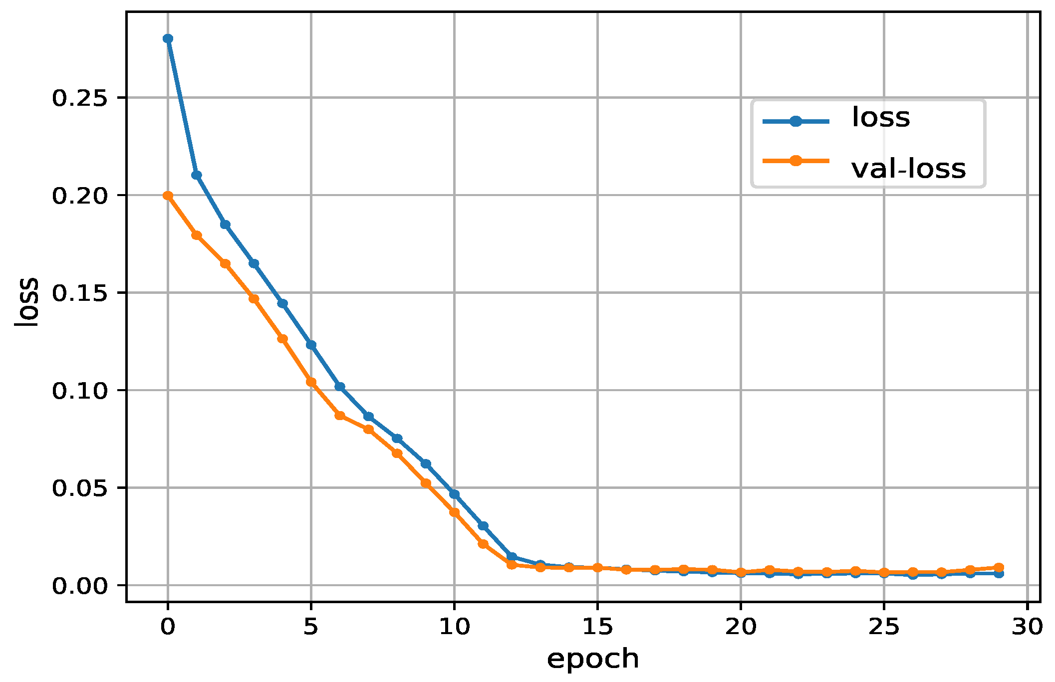
Using the best hyperparameter settings, i.e., , and , we draw the loss as a function of the epoch. In Figure 4, the loss and the val-loss represent the values of the loss function in the training set and the validation set, respectively. As can be seen in Figure 4, our proposed approach has a fast convergence performance and a high degree of accuracy. More clearly, after 10 epochs, the loss and the val-loss converge to 0.0038 and 0.0052, respectively. One can found that there is a difference in the magnitude of the MAE in Figure 4 and tables in Section 4.1.1. The reason for this situation is the use of the Min-Max Normalization. To be more specific, the features were scaled before being fed into the proposed algorithm. The MAEs in Figure 4 were calculated according to the normalized data. In the experiment, the features were scaled to lie between zero and one, resulting in small values of the MAE. It should be noted that, when the training process was finished, the predicted values were transformed inversely to the original range to compare to the actual values. The MAEs shown in the tables in Section 4.1.1 were calculated after the reverse process. Thus, relatively large values were obtained. Intuitively, Figure 5 shows the comparison of the output of the proposed train dynamic model and the original data. The raw features, i.e., , , and , were directly fed into the proposed model to get the the train speed of the next time step. Thus, it can be considered as predicting train speed for one-step ahead. As can be seen in Figure 5, no matter how the operation process changes (such as train accelerating and train braking), the output of the proposed approach is particularly close to the original data.
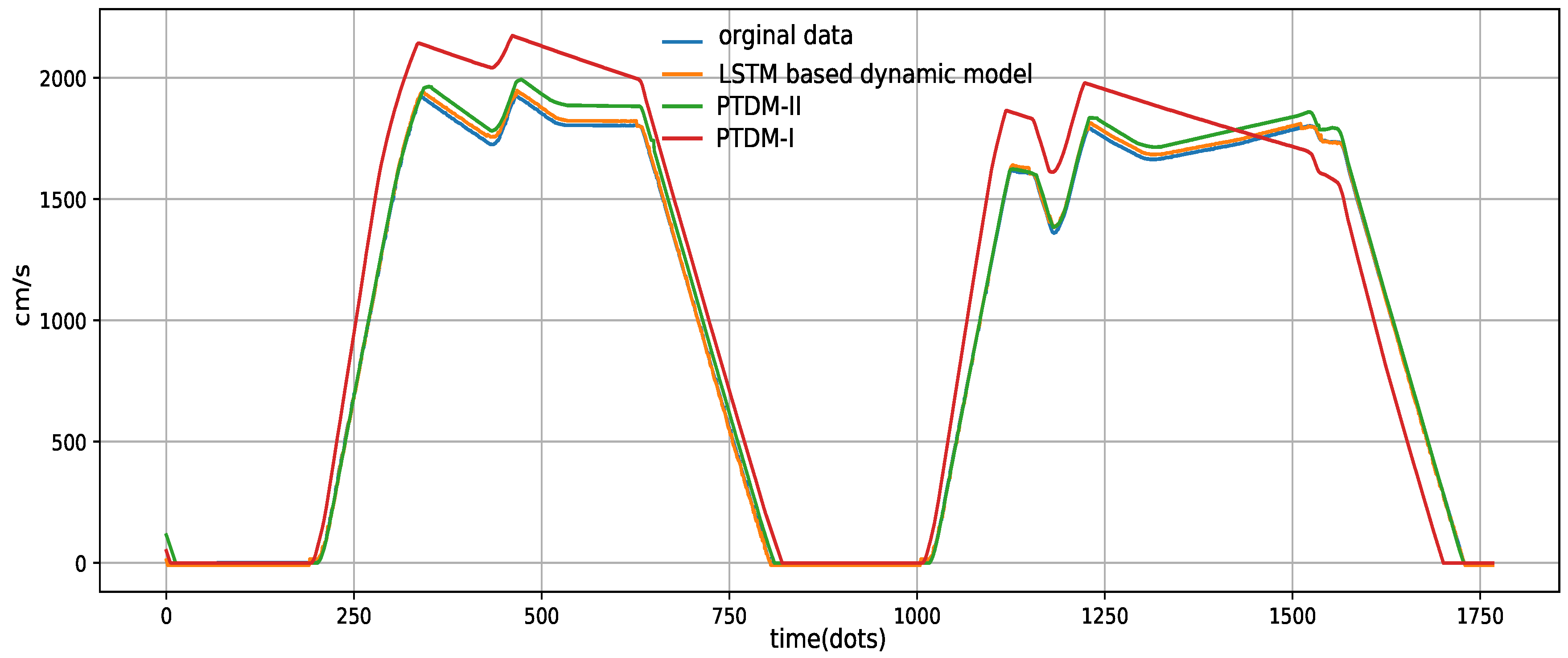
To further verify the effectiveness of the proposed train dynamic model, we also made a comparison with another two parametric approaches: (i) a parametric train dynamic model that is currently being used in real train control systems (PTDM-I); and (ii) a parametric approach that the parameters have been optimized using the fruit fly optimization algorithm (PTDM-II). Note that these two approaches follow the single-point train dynamic model as described in Section 3.1. The PTDM-I relies on a simple method of table lookups to produce the speed of the next time step. The corresponding relationship between the velocity (km/h) and the acceleration (m/s) of PTDM-I is shown in Table 5. PTDM-II uses the fruit fly optimization algorithm to optimize the resistance parameters of the Davis formula, i.e., , and , as shown in Equation (2). The settings of these parameters for Yanfang Metro Line are listed in Table 6.
The comparison results of the LSTM based train dynamic model, PTDM-I, PTDM-II and the original data are presented in Figure 6. We only draw the operation curves of these approaches from Xingcheng Station to Magezhuang Station for clarity. As expected, the proposed dynamic model clearly outperformed two traditional parametric models: PTDM-I and PTDM-II. As can be seen in Figure 6, PTDM-I has the highest output errors. In actual applications, before launching a new metro line, the relational table should be adjusted by experienced engineers to adapt to the real environment. As an optimized version of PTDM-I, the model performance was significantly improved in PTDM-II. The reason is that the parameters were tuned using the fruit fly optimization algorithm. More specifically, for each station interval, this algorithm was repeatedly employed for parameter optimization. For example, according to Table 6, , and are, respectively, adjusted as 2.908890237, 0.014551371 and 0.00002373932 from Caoziwu Station to Yancun Station. Furthermore, these parameters change to 1.078270769, 0.005545171 and 0.0003830150 between Yancun Station and Xingcheng station. The fruit fly optimization algorithm belongs to a kind of interactive evolutionary computation (refer to [54] for more information). However, PTDM-II is shown to be less effective in the train coasting phase and the train cruising phase. One can also find that the performance of the proposed model was better than PTDM-II in the train coasting phase and the train cruising phase due to its learning ability. Similar to Figure 5, the proposed model could generate very close output to the original data. The experimental results demonstrate that the LSTM based model could remarkably enhance the output accuracy compared to the parametric based models.
4.2. Results of n Steps Speed Prediction
By employing the feature engineering, delicate descriptions of the raw features can be obtained. With the captured long-term pattern of the data and inspired by the studies on traffic speed prediction [41,42,43], we extended the LSTM based approach to predict train speed for multi-step ahead. With the help of the train speed prediction, the train running status can be obtained proactively. According to the predicted output, automatic train operation systems or drivers may take actions in advance to avoid or reduce damage resulting from system abnormalities. Taking the emergency braking distance and the sample interval into consideration, in the experiments, we predicted the 10-step ahead ( s), 30-step ahead ( s) and 50-step ahead ( s) train speeds.
Table 7 provides the MAE and MSE with different prediction steps. By observing Table 7 and the tables in Section 4.1.1, one can find that the MAE and MSE values for multi-step ahead are significantly larger than the results of one-step ahead, i.e, the proposed dynamic model. As the prediction time step increases, the prediction accuracy of train speed deteriorates. For a long-term prediction (), values of the MAE and MSE are 101.36 and 13,281.65, respectively. This can be understood by the fact that the increase of the prediction step may add more uncertainties, which leads to a reduction of the prediction performance.
Taking 30-step-ahead prediction as an example, we draw the loss as a function of the epoch in Figure 7. Similar to Figure 4, the loss and the val-loss represent the values of the loss function in the training set and the validation set, respectively. The settings of the hyperparameters in Figure 7 and Table 7 are exactly the same as the settings in Section 4.1.2. It was observed that the loss oscillates at 0.023 and the val-loss converges to 0.039 after 70 epochs.
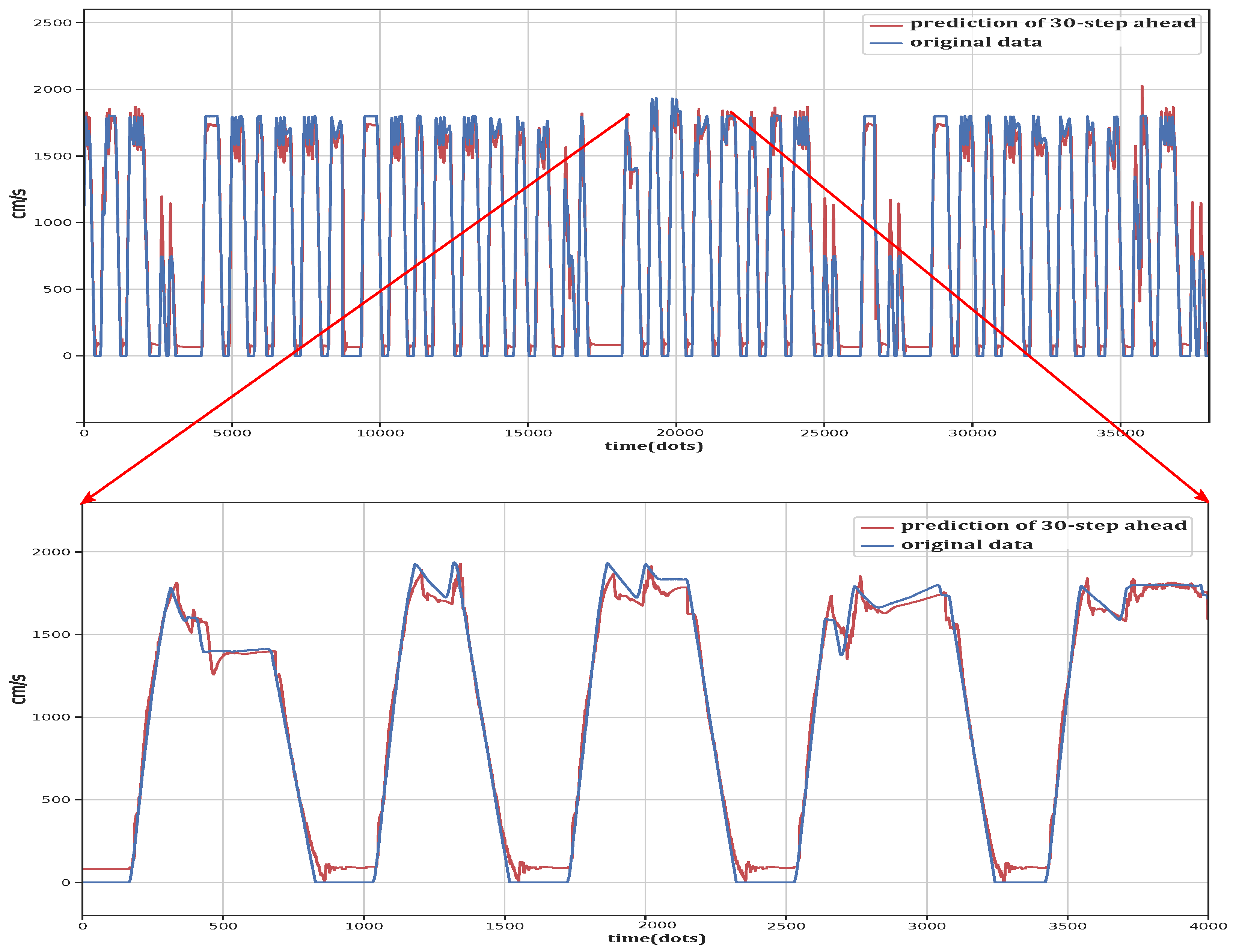
To further examine the prediction performance in a more intuitive way, the comparisons between the original data and the output of 10-step-ahead prediction, 30-step-ahead prediction and 50-step-ahead prediction are shown in Figure 8, Figure 9 and Figure 10, respectively. The algorithm output of 10-step-ahead prediction was observed to be relatively close to the original data. As the time step increases, the difference between the predicted value and the original data becomes larger, which is consistent with the results in Table 7. One can notice that the prediction accuracy degenerates after certain turning points. The reason is that the features extracted from the previous data may not describe the rapid change of the train speed. As can be seen in Figure 8, Figure 9 and Figure 10, although the error increases in these scenarios, the proposed method has the ability to predict train speed since the prediction error is controlled to a legitimate range. The software program will be made available in the open code. One can found the link in the Supplementary Materials.
5. Conclusions
In this paper, based on an LSTM neural network, a data-driven method is developed to build the train dynamic model and predict the train speed. Different from the parametric approaches, the proposed method is more adaptive to the real environment due to its strong knowledge expression ability and learning ability. To make fair comparisons with other models, the same inputs as the parametric approaches (analog output, traction brake, rail slope and train speed) were fed to the LSTM based algorithm, after data preprocessing and feature engineering. The hyperparameters of the proposed algorithm were carefully tuned to improve the output accuracy. The performance of the proposed method was evaluated in terms of three measurement criteria: MAE, MSE, and R2. Using the actual data collected from Shenzhen Metro Line No. 7 and Beijing Yanfang Metro Line in China, the proposed model was compared with two traditional parametric approaches: PTDM-I and PTDM-II. The comparison results demonstrate that the model performance was remarkably enhanced compared to these algorithms. By combining lagged features and statistical features, the LSTM based method was then extended to predict train speed for a longer period of time. Experimental results suggest that the extended version can be applied to solve the train speed prediction problem since the prediction errors are well controlled.
However, there are still some shortcomings in the proposed method. Firstly, since lagged features are employed in the proposed algorithm, high prediction errors may be produced in the beginning phase. It would be useful to improve the proposed algorithm by solving the initialization problem. Secondly, the on-board devices in urban rail transit have the characteristics of limited hardware and low-complexity. How to reduce the complexity of the proposed algorithm is a major concern for future studies.
Supplementary Materials
The open code file is available online at https://drive.google.com/open?id=1amXoTR6Tr3bdq1khkU-B6_fhjJ0po9rp.
Author Contributions
Conceptualization, T.T. and C.G.; formal analysis, T.T. and Z.L.; methodology, T.T. and Z.L.; writing—original draft, Z.L.; validation, Z.L.; resources, C.G.; supervision, C.G.
Funding
This research was funded by Beijing Postdoctoral Research Foundation.
Conflicts of Interest
We declare that we have no financial or personal relationships with other people or organizations that could inappropriately influence our work. There is no professional or other personal interest of any nature or kind in any product, service and/or company that could be construed as influencing the position presented in, or the review of, the manuscript entitled.
References
- Famurewa, S.M.; Zhang, L.; Asplund, M. Maintenance analytics for railway infrastructure decision support. J. Qual. Maint. Eng. 2017, 23, 310–325. [Google Scholar] [CrossRef]
- Cacchiani, V.; Huisman, D.; Kidd, M.; Kroon, L.; Toth, P.; Veelenturf, L.; Wagenaar, J. An overview of recovery models and algorithms for real-time railway rescheduling. Transp. Res. Part B 2014, 63, 15–37. [Google Scholar] [CrossRef] [Green Version]
- Leung, P.; LEE, C.M.; Eric, W.M. Estimation of electrical power consumption in subway station design by intelligent approach. Appl. Energy 2013, 101, 634–643. [Google Scholar] [CrossRef]
- Khmelnitsky, E. On an optimal control problem of train operation. IEEE Trans. Autom. Control 2000, 45, 1257–1266. [Google Scholar] [CrossRef]
- Kiencke, U.; Nielsen, L.; Sutton, R.; Schilling, K.; Papageorgiou, M.; Asama, H. The impact of automatic control on recent developments in transportation and vehicle systems. Annu. Rev. Control 2006, 30, 81–89. [Google Scholar] [CrossRef]
- Song, Q.; Song, Y.; Tang, T.; Ning, B. Computationally Inexpensive Tracking Control of High-Speed Trains With Traction/Braking Saturation. IEEE Trans. Intell. Transp. Syst. 2011, 12, 1116–1125. [Google Scholar] [CrossRef]
- Albrecht, A.; Howlett, P.; Pudney, P.; Xuan, V.; Zhou, P. The key principles of optimal train control—Part 2: Existence of an optimal strategy, the local energy minimization principle, uniqueness, computational techniques. Transp. Res. Part B 2015, 94, 509–538. [Google Scholar] [CrossRef]
- Wang, P.; Goverde, R.M.P. Multiple-phase train trajectory optimization with signalling and operational constraints. Transp. Res. Part C 2016, 69, 255–275. [Google Scholar] [CrossRef]
- Quaglietta, E.; Pellegrini, P.; Goverde, R.M.P.; Albrecht, T. The ON-TIME real-time railway traffic management framework: A proof-of-concept using a scalable standardised data communication architecture. Transp. Res. Part C 2016, 63, 23–50. [Google Scholar] [CrossRef]
- Faieghi, M.; Jalali, A.; Mashhadi, S.K. Robust adaptive cruise control of high speed trains. ISA Trans. 2014, 53, 533–541. [Google Scholar] [CrossRef]
- Gao, S.; Dong, H.; Ning, B.; Sun, X.B. Neural adaptive control for uncertain MIMO systems with constrained input via intercepted adaptation and single learning parameter approach. Nonlinear Dyn. 2015, 82, 1–18. [Google Scholar] [CrossRef]
- Astolfi, A.; Menini, L. Input/output decoupling problems for high speed trains. In Proceedings of the 2002 American Control Conference (IEEE Cat. No. CH37301), Anchorage, AK, USA, 8–10 May 2002. [Google Scholar]
- Dong, H.R.; Gao, S.G.; Ning, B.; Li, L. Extended fuzzy logic controller for high speed train. Neural Comput. Appl. 2013, 22, 321–328. [Google Scholar] [CrossRef]
- Tang, J.; Liu, F.; Zou, Y.J.; Zhang, W.B.; Wang, Y.H. An Improved Fuzzy Neural Network for Traffic Speed Prediction Considering Periodic Characteristic. IEEE Trans. Intell. Transp. Syst. 2017, 18, 1–11. [Google Scholar] [CrossRef]
- Altche, F.; Arnaud, D.L.F. An LSTM network for highway trajectory prediction. In Proceedings of the 2017 IEEE 20th International Conference on Intelligent Transportation Systems (ITSC), Yokohama, Japan, 16–19 October 2017; pp. 353–359. [Google Scholar]
- Ma, X.; Dao, Z.; He, Z.; Ma, J.; Wang, Y.; Wang, Y. Learning Traffic as Images: A Deep Convolutional Neural Network for Large-Scale Transportation Network Speed Prediction. Sensors 2017, 17, 818. [Google Scholar] [CrossRef] [PubMed]
- Sun, H.; Hou, Z.; Li, D. Coordinated Iterative Learning Control Schemes for Train Trajectory Tracking with Overspeed Protection. IEEE Trans. Autom. Sci. Eng. 2013, 10, 323–333. [Google Scholar] [CrossRef]
- Chen, D.; Gao, C. Soft computing methods applied to train station parking in urban rail transit. Appl. Soft Comput. 2012, 12, 759–767. [Google Scholar] [CrossRef]
- Zhang, C.Y.; Chen, D.; Yin, J.; Chen, L. Data-driven train operation models based on data mining and driving experience for the diesel-electric locomotive. Adv. Eng. Inform. 2016, 30, 553–563. [Google Scholar] [CrossRef]
- Hochreiter, S.; Schmidhuber, J. Long Short-Term Memory. Neural Comput. 1997, 9, 1735–1780. [Google Scholar] [CrossRef]
- Howlett, P. Optimal strategies for the control of a train. Automatica 1996, 32, 519–532. [Google Scholar] [CrossRef]
- Liu, R.; Golovitcher, I.M. Energy-efficient operation of rail vehicles. Transp. Res. Part A 2003, 37, 917–932. [Google Scholar] [CrossRef]
- Wang, Y.; De Schutter, B.; van den Boom, T.J.; Ning, B. Optimal trajectory planning for trains. A pseudospectral method and a mixed integer linear programming approach. Transp. Res. Part C 2013, 29, 97–114. [Google Scholar] [CrossRef]
- Su, S.; Li, X.; Tao, T.; Gao, Z. A Subway Train Timetable Optimization Approach Based on Energy-Efficient Operation Strategy. IEEE Trans. Intell. Transp. Syst. 2013, 14, 883–893. [Google Scholar] [CrossRef]
- Su, S.; Tang, T.; Roberts, C. A Cooperative Train Control Model for Energy Saving. IEEE Trans. Intell. Transp. Syst. 2015, 16, 622–631. [Google Scholar] [CrossRef]
- Gruber, P.; Bayoumi, M. Suboptimal control strategies for multilocomotive powered trains. IEEE Trans. Autom. Control 1982, 27, 536–546. [Google Scholar] [CrossRef]
- Chou, M.; Xia, X.; Kayser, C. Modelling and model validation of heavy-haul trains equipped with electronically controlled pneumatic brake systems. Control Eng. Pract. 2007, 15, 501–509. [Google Scholar] [CrossRef]
- Zhuan, X.; Xia, X. Speed regulation with measured output feedback in the control of heavy haul trains. Automatica 2008, 44, 242–247. [Google Scholar] [CrossRef]
- Song, Q.; Song, Y.D. Data-based fault-tolerant control of high-speed trains with traction/braking notch nonlinearities and actuator failures. IEEE Trans. Neural Netw. 2011, 22, 2242–2250. [Google Scholar] [CrossRef]
- Li, S.; Yang, L.; Li, K.; Gao, Z. Robust sampled-data cruise control scheduling of high speed train. Transp. Res. Part C 2014, 46, 274–283. [Google Scholar] [CrossRef]
- Zhang, J.; Wang, F.; Wang, K.; Lin, W.; Xu, X.; Chen, C. Data-Driven Intelligent Transportation Systems: A Survey. IEEE Trans. Intell. Transp. Syst. 2011, 12, 1624–1639. [Google Scholar] [CrossRef]
- Ji, Z. Applications of machine learning methods in problem of precise train stopping. Comput. Eng. Appl. 2006, 46, 226–230. [Google Scholar]
- Chen, D.; Chen, R.; Li, Y.; Tang, T. Online Learning Algorithms for Train Automatic Stop Control Using Precise Location Data of Balises. IEEE Trans. Intell. Transp. Syst. 2013, 14, 1526–1535. [Google Scholar] [CrossRef]
- Radac, M.B.; Precup, R.E. Data-Driven Model-Free Tracking Reinforcement Learning Control with VRFT-based Adaptive Actor-Critic. Appl. Sci. 2019, 9, 1807. [Google Scholar] [CrossRef]
- Chen, H.; Jiang, B.; Chen, W.; Yi, H. Data-driven Detection and Diagnosis of Incipient Faults in Electrical Drives of High-Speed Trains. IEEE Trans. Ind. Electron. 2019, 66, 4716–4725. [Google Scholar] [CrossRef]
- Ma, X.; Tao, Z.; Wang, Y.; Yu, H.; Wang, Y. Long short-term memory neural network for traffic speed prediction using remote microwave sensor data. Transp. Res. Part C 2015, 54, 187–197. [Google Scholar] [CrossRef]
- Shi, X.; Shao, X.; Guo, Z.; Wu, G.; Zhang, H.; Shibasaki, R. Pedestrian Trajectory Prediction in Extremely Crowded Scenarios. Sensors 2019, 19, 1223. [Google Scholar] [CrossRef] [PubMed]
- Yin, H.; Wong, S.C.; Xu, J.; Wong, C.K. Urban traffic flow prediction using a fuzzy-neural approach. Transp. Res. Part C 2002, 10, 85–98. [Google Scholar] [CrossRef]
- Asif, M.T.; Dauwels, J.; Chong, Y.; Oran, A.; Jaillet, P. Spatiotemporal Patterns in Large-Scale Traffic Speed Prediction. IEEE Trans. Intell. Transp. Syst. 2014, 15, 794–804. [Google Scholar] [CrossRef]
- Savvopoulos, A.; Kanavos, A.; Mylonas, P.; Sioutas, S. LSTM Accelerator for Convolutional Object Identification. Algorithms 2018, 11, 157. [Google Scholar] [CrossRef]
- Duan, Y.; Lv, Y.S.; Wang, F.Y. Travel time prediction with LSTM neural network. In Proceedings of the 2016 IEEE 19th International Conference on Intelligent Transportation Systems (ITSC), Rio de Janeiro, Brazil, 1–4 November 2016. [Google Scholar]
- Chen, Y.Y.; Lv, Y.S.; Li, Z.J.; Wang, F.Y. Long short-term memory model for traffic congestion prediction with online open data. In Proceedings of the 2016 IEEE 19th International Conference on Intelligent Transportation Systems (ITSC), Rio de Janeiro, Brazil, 1–4 November 2016. [Google Scholar]
- Cui, Z.; Ke, R.; Wang, Y. Deep Bidirectional and Unidirectional LSTM Recurrent Neural Network for Network-wide Traffic Speed Prediction. arXiv 2018, arXiv:1801.02143. [Google Scholar]
- Yin, J.; Tang, T.; Yang, L.; Xun, J.; Gao, Z. Research and development of automatic train operation for railway transportation systems: A survey. Transp. Res. Part C 2017, 85, 548–572. [Google Scholar] [CrossRef]
- Dhahbi, S.; Abbas-Turki, A.; Hayat, S.; Moudni, A. Study of the high-speed trains positioning system: European signaling system ERTMS/ETCS. In Proceedings of the 2011 4th International Conference on Logistics, Hammamet, Tunisia, 31 May–3 June 2011. [Google Scholar]
- Gers, F.A. Learning to forget: Continual prediction with LSTM. In Proceedings of the International Conference on Artificial Neural Networks, Edinburgh, UK, 7–10 September 1999. [Google Scholar]
- Bengio, Y. Learning Long-term Dependencies With Gradient Descent is Difficult. IEEE Trans. Neural Netw. 2002, 5, 157–166. [Google Scholar] [CrossRef] [PubMed]
- Le, Q.V.; Jaitly, N.; Hinton, G.E. A Simple Way to Initialize Recurrent Networks of Rectified Linear Units. arXiv 2015, arXiv:1504.00941. [Google Scholar]
- Park, D.; Rilett, L.R. Forecasting freeway link travel times with a multilayer feedforward neural network. Comput.-Aided Civ. Infrastruct. Eng. 2010, 14, 357–367. [Google Scholar] [CrossRef]
- Kingma, D.P.; Ba, J. Adam: A method for stochastic optimization. arXiv 2014, arXiv:1412.6980. [Google Scholar]
- Phillips, D.J.; Wheeler, T.A.; Kochenderfer, M.J. Generalizable intention prediction of human drivers at intersections. In Proceedings of the 2017 IEEE Intelligent Vehicles Symposium (IV), Los Angeles, CA, USA, 11–14 June 2017. [Google Scholar]
- Greff, K.; Srivastava, R.K.; Koutnik, J.; Steunebrink, B.R.; Schmidhuber, J. LSTM: A Search Space Odyssey. IEEE Trans. Neural Netw. Learn. Syst. 2016, 28, 2222–2232. [Google Scholar] [CrossRef] [PubMed]
- Swami, A.; Jain, R. Scikit-learn: Machine Learning in Python. J. Mach. Learn. Res. 2013, 12, 2825–2830. [Google Scholar]
- Pan, W.T. A new Fruit Fly Optimization Algorithm: Taking the financial distress model as an example. Knowl.-Based Syst. 2012, 26, 69–74. [Google Scholar] [CrossRef]
Figure 1.
Parametric based train dynamic model.

Figure 2.
The internal structure of an LSTM cell.

Figure 3.
Raw features.

Figure 4.
Comparison of the loss in the training results.

Figure 5.
Comparison of the original data and the output of the proposed model.

Figure 6.
Comparison of different approaches.

Figure 7.
Comparison of the loss for 30-step-ahead prediction.

Figure 8.
Comparison of the original data and the output of 10-step-ahead prediction.

Figure 9.
Comparison of the original data and the output of 30-step-ahead prediction.

Figure 10.
Comparison of the original data and the output of 50-step-ahead prediction.


Table 1.
Illustration of parameters in the LSTM network structure.
| Variable Name | Explanation | Type |
|---|---|---|
| output of input gate at tth time step | vector | |
| weight matrix of input gate | matrix | |
| output of the recurrent hidden layer at tth time step | vector | |
| bias vector of the input gate | vector | |
| activation function of input gate | function | |
| dimension of the recurrent hidden layer input | integer | |
| dimension of the recurrent hidden layer output | integer | |
| dimension of the state vector | integer | |
| output of forget gate at tth time step | vector | |
| weight matrix of forget gate | matrix | |
| bias vector of forget gate | vector | |
| activation function of forget gate | function | |
| output of output gate at tth time step | vector | |
| weight matrix of output gate | matrix | |
| bias vector of output gate | vector | |
| activation function of output gate | function | |
| state update vector at tth time step | vector | |
| weight matrix of state update vector | matrix | |
| bias vector of state update vector | vector | |
| current cell state vector at tth time step | vector |
Table 2.
Train operation information saved by Vehicle On Board Controller.
| Time | System | Number | Data Integrity | Driving Condition | Offset | Train Speed |
|---|---|---|---|---|---|---|
| 20:20:57 | 4646 | 332,071 | True | 2 | 1292 | 1037 |
| Number of current station | Number of next station | Link | Distance | Run level | Slope | |
| 35 | 36 | 177 | 11,659 | 3 | 0 | |
| Analog output | Speed limit | Traction braking | Network voltage | Network flow | Load | |
| 134 | 1054 | 1 | 868 | 303 | 23 | |
Table 3.
Influence of the hidden size and the batch size.
| (a) Performance Comparison with Different Hidden Sizes. | |||
| Hidden Size | MSE | MAE | R2 |
| 2 | 4454.57 | 44.1 | 0.9878 |
| 6 | 318.88 | 13.8 | 0.9991 |
| 10 | 195.67 | 9.55 | 0.9991 |
| 14 | 225.64 | 12.32 | 0.9969 |
| 71.75 | 6.07 | 0.9997 | |
| 22 | 334.02 | 13.93 | 0.9981 |
| 26 | 201.52 | 12.09 | 0.9990 |
| 30 | 267.38 | 12.56 | 0.9985 |
| (b) Performance Comparison with Different Batch Sizes. | |||
| Batch Size | MSE | MAE | R2 |
| 32 | 350.92 | 16.45 | 0.9990 |
| 64 | 191.53 | 10.17 | 0.9994 |
| 124.53 | 8.42 | 0.9996 | |
| 256 | 178.99 | 9.95 | 0.9994 |
| 512 | 665.60 | 17.73 | 0.9981 |
| 768 | 859.31 | 20.49 | 0.9976 |
| 1024 | 1688.47 | 27.84 | 0.9953 |
| 1280 | 9992.88 | 68.55 | 0.9767 |
| 1536 | 14,986.28 | 309.58 | 0.3254 |
Table 4.
Influence of the learning rate and the number of layers.
| (a) Performance Comparison with Different Learning Rates. | ||
| Learning Rate | MSE | MAE |
| 8940.12 | 114.69 | |
| 518.34 | 18.18 | |
| 403.57 | 15.99 | |
| 122.93 | 9.28 | |
| 491.82 | 17.29 | |
| 2035.62 | 40.39 | |
| (b) Performance Comparison with Different Numbers of Hidden Layers. | ||
| Number of Hidden Layers | MSE | MAE |
| 165.19 | 9.04 | |
| 2 | 194.19 | 10.31 |
| 3 | 482.25 | 15.04 |
Table 5.
Relationship between the velocity and the acceleration of PTDM-I.
| Velocity | Acceleration | Velocity | Acceleration | Velocity | Acceleration | Velocity | Acceleration |
|---|---|---|---|---|---|---|---|
| 3 | 1.081497 | 5 | 1.113422 | 7 | 1.113031 | 9 | 1.112617 |
| 11 | 1.112179 | 13 | 1.111718 | 15 | 1.111233 | 17 | 1.110725 |
| 19 | 1.110193 | 21 | 1.109638 | 23 | 1.109059 | 25 | 1.108456 |
| 27 | 1.107831 | 29 | 1.107181 | 31 | 1.106508 | 33 | 1.105811 |
| 35 | 1.105091 | 37 | 1.104348 | 39 | 1.10358 | 41 | 1.10279 |
| 43 | 1.101975 | 45 | 1.101138 | 47 | 1.100276 | 49 | 1.099391 |
| 51 | 1.098483 | 53 | 1.097551 | 55 | 1.096595 | 57 | 1.095616 |
| 59 | 1.094614 | 61 | 1.093587 | 63 | 1.074573 | 65 | 0.9804486 |
| 67 | 0.950206 | 69 | 0.893474 | 71 | 0.8668448 | 73 | 0.8167437 |
| 75 | 0.7704815 | 77 | 0.7276618 | 79 | 0.6879385 | 81 | 0.6335031 |
Table 6.
Parameter settings of PTDM-II.
| Station Interval | |||
|---|---|---|---|
| 1.051400712 | 0.005980156 | 0.00022866 | |
| 2.908890237 | 0.014551371 | 0.00002373932 | |
| 1.078270769 | 0.005545171 | 0.0003830150 | |
| 1.634758136 | 0.026648264 | 0.0000319240 | |
| 1.051565386 | 0.020496939 | 0.0000288589 | |
| 1.022215526 | 0.005227106 | 0.00002196136 | |
| 1.035460959 | 0.006413686 | 0.000698753 | |
| 1.039279709 | 0.005581798 | 0.000388984 |
Table 7.
Prediction accuracy with different prediction steps.
| Evaluation Indicator | |||
|---|---|---|---|
| 31.70 | 38.43 | 101.36 | |
| 2607.12 | 7492.34 | 13281.65 |
© 2019 by the authors. Licensee MDPI, Basel, Switzerland. This article is an open access article distributed under the terms and conditions of the Creative Commons Attribution (CC BY) license (http://creativecommons.org/licenses/by/4.0/).
Share and Cite
MDPI and ACS Style
Li, Z.; Tang, T.; Gao, C. Long Short-Term Memory Neural Network Applied to Train Dynamic Model and Speed Prediction. Algorithms 2019, 12, 173. https://0-doi-org.brum.beds.ac.uk/10.3390/a12080173
AMA Style
Li Z, Tang T, Gao C. Long Short-Term Memory Neural Network Applied to Train Dynamic Model and Speed Prediction. Algorithms. 2019; 12(8):173. https://0-doi-org.brum.beds.ac.uk/10.3390/a12080173
Chicago/Turabian StyleLi, Zhen, Tao Tang, and Chunhai Gao. 2019. "Long Short-Term Memory Neural Network Applied to Train Dynamic Model and Speed Prediction" Algorithms 12, no. 8: 173. https://0-doi-org.brum.beds.ac.uk/10.3390/a12080173
Note that from the first issue of 2016, this journal uses article numbers instead of page numbers. See further details here.