A Fast Particle-Locating Method for the Arbitrary Polyhedral Mesh

Abstract

A fast particle-locating method is proposed for the hybrid Euler–Lagrangian models on the arbitrary polyhedral mesh, which is of essential importance to improve the computational efficiency by searching the host cells for the tracked particles very efficiently. A background grid, i.e., a uniform Cartesian grid with a grid spacing much smaller than computational mesh, is constructed over the whole computational domain. The many-to-many mapping relation between the computational mesh and the background grid is then specified through a recursive tetrahedron neighbor searching procedure, after the tetrahedral decomposition of computational cells and a mapping inverse operation. Finally, the host cell is straightforwardly identified by the point-in-cell test among the optional elements determined based on the mapping relation. The proposed method is checked on three meshes with different types of the cells and compared with the existing methods in the literatures. The results reveal that the present method is highly efficient and easy to implement on the arbitrary polyhedral mesh.

1. Introduction

The hybrid Euler–Lagrangian models are widely used in simulating the flows in the dispersed systems. In these models, the continuous phase is described through spatial field distribution in Eulerian framework, while the dispersed phase is considered through tracking the movements of the dispersed phase entities (particles, bubbles, or droplets, which we shall call particles collectively). During simulations, the interactions between continuous and dispersed phases are realized by computing the movements of the particles using the own parameters at the particle centers and evaluating the effect of the particles (in terms of their volumes, velocities, and so on) on the dynamic behaviors of the continuous phase. As a result, locating the host cell of each particle at every time step is required. Although locating the host cell on a uniform Cartesian mesh is easy, it is not the case for the unstructured meshes, especially for those with the arbitrary polyhedral cells, where the particle locating is usually a time-consuming task and brings a heavy burden on the overall computational efficiency. In previous studies [1,2], it was found a faster particle-locating method is necessary for simulations within the complex geometries using the arbitrary polyhedral meshes.

Several methods have been proposed for the particle locating on irregular meshes. Existing methods can be categorized into two types, i.e., the known vicinity face-to-face searching methods, such as Chen and Pereira [3], Vaidya et al. [4], Haselbacher et al. [5], Macpherson et al. [6], Ke et al. [7], Capodaglio [8], and Stuart et al. [9], among others, and the auxiliary grid methods, such as Seldner and Westermann [10], Muradoglu and Kayaalp [11], Martin et al. [12], and Jin et al. [13], among others. Using the known vicinity face-to-face searching methods, a starting point along with its host cell as the starting host cell is given for each tracked particle at first. The point-in-cell test is conducted in the starting host cell at first and then carried out in one of its neighbor cells, determined by some prescribed rules if the starting host cell does not contain the particle. This procedure continues until the host cell is found [14]. The computational efficiency of the known vicinity face-to-face searching method highly depends on the choice of the starting point. Unfortunately, it is difficult to find the optimal starting point to lower the computational expense. The auxiliary grid methods construct a regular background grid, e.g., a tree-type grid or a uniform Cartesian grid with a larger grid spacing than that of the computational mesh, to efficiently locate the host cells for tracked particles. The mapping relation between the background grid and computational mesh is specified before the simulation. It stores, for each background cell, the indices of the several computational cells which are fully or partially contained by the background cell are found. The particle is located within a background cell at first, and then the point-in-cell tests are conducted within only several computational cells related to that background cell to determine the host cell. Since locating the particle on a regular background grid is considerably simple and the point-in-cell tests are only conducted in several most possible cells, the computational efficiency of particle locating is significantly improved by using an auxiliary regular grid.

So far, the auxiliary grid method with a uniform background grid has been used for particle locating on two-dimensional curvilinear mesh [11,12]. In this study, we extend the auxiliary grid method to the three-dimensional arbitrary polyhedral mesh, which is a practical choice for numerical simulations in complex geometries and more challenging for particle-locating methods. Furthermore, we study the influence of the resolution of the background grid on the performance of the particle-locating method. Different from the existing studies, we introduce a uniform Cartesian background grid with much smaller grid spacing than that of the computational mesh. As a result, many background cells are related to just one computational cell, and the point-in-cell test is unnecessary if the particle is located within one of those background cells. This new algorithm is named as PLUG (an abbreviation of Point Locating with Uniform Grid) method.

The rest of this paper is organized as follows. A detailed description of PLUG method is given in Section 2. A numerical test is carried out in Section 3 to check the performance of the proposed method and make comparison with the existing particle-locating methods. Finally, a short summary is given in Section 4.

2. PLUG Method

The procedure to determine the host cells for the particles using the PLUG method includes three steps as follows:

Step one: building a regular background grid, which is a uniform Cartesian grid with the prescribed resolution over the whole computational domain.

Step two: specifying the mapping relation between the background cells and the computational cells which store, for each background cell, the indices of the computational cells containing or partially overlapping with it.

Step three: locating the particle on the background grid and conducting the point-in-cell test to determine the host cell if necessary.

2.1. Background Grid

A uniform Cartesian grid is adopted in the present study to be the background grid. The background grid should cover the whole computational domain as

$$D=\left[x_{\min }-\delta ,x_{\max }+\delta \right]\times \left[y_{\min }-\delta ,y_{\max }+\delta \right]\times \left[z_{\min }-\delta ,z_{\max }+\delta \right],$$

(1)

where x_min, y_min, and z_min are minimal values of x, y, and z coordinates of the computational domain, x_max, y_max, and z_max are corresponding maximal values, and $\delta$ is a small positive number to assure that the background grid completely covers the whole computational domain.

A uniform grid is constructed by prescribing the number of elements in three directions, i.e., n_x, n_y, and n_z. As a result, the grid spacings in different directions are

$$\Delta x=\frac{x_{\max }-x_{\min }}{n_x},\Delta y=\frac{y_{\max }-y_{\min }}{n_y} and \Delta z=\frac{z_{\max }-z_{\min }}{n_z}$$

(2)

For a particle centered at point P (x_p, y_p, z_p), the index of background cell containing the point P (${\tilde{C}}_{ijk}$, the host cell on the background grid) is easily determined as

$$\left(i,j,k\right)=\left[\mathrm{int}\left(x_p-x_{\min },\Delta x\right),\mathrm{int}\left(y_p-y_{\min },\Delta y\right),\mathrm{int}\left(z_p-z_{\min },\Delta z\right)\right],$$

(3)

where the function int (x, y) gives the maximal integer smaller than x/y.

For sake of brevity, this three-dimensional index (i, j, k) can be replaced by a one-dimensional index I as

$$I=n_y{n}_{z}i+n_{z}j+k,$$

(4)

and the inverse transformation is accomplished by

$$i=\mathrm{int}[\mathrm{int}\left(I,n_z\right),n_y],j=\mathrm{mod}\left[\mathrm{int}\left(I,n_z\right),n_y\right] \mathrm{and} z=\mathrm{mod}\left(I,n_z\right),$$

(5)

where the function mod (a, b) is the remainder operator for two integers a and b.

2.2. Mapping Relation Between Background Cells and Computational Cells

As shown in (3), the particle locating on the background grid is straightforward. Thus, the key task in the present study is to find the mapping relation between the background cubes and the computational cells. Please note the term “cube” will be used to denote the cells on background grid hereafter to distinguish from computational cells. As mentioned above, the mapping relation should give a integer array [a_I1, a_I2, …, a_Is] for any background cube ${\tilde{C}}_I$, which are the indices of a set of the computational cells [C_aI1, C_aI2, …, C_aIs] containing or partially overlapping with the corresponding background cube, i.e., satisfying

$$S_{aIq}\cap {\tilde{S}}_I\ne 0\left(q=0 \mathrm{to} s\right),$$

(6)

where S_aIq is the volume covered by the computational cell C_Iq and ${\tilde{S}}_I$ is the volume covered by background cube ${\tilde{C}}_I$. For some background cells, there is a computational cell overlapping with them. Thus, the q should start from zero in Equation (6).

Considering all the background cubes, a list cube2cell can be obtained, with each component being the above array for the corresponding background cube. The length of the list cube2cell equals the total number of the background cubes, and parameter s is different for different background cube.

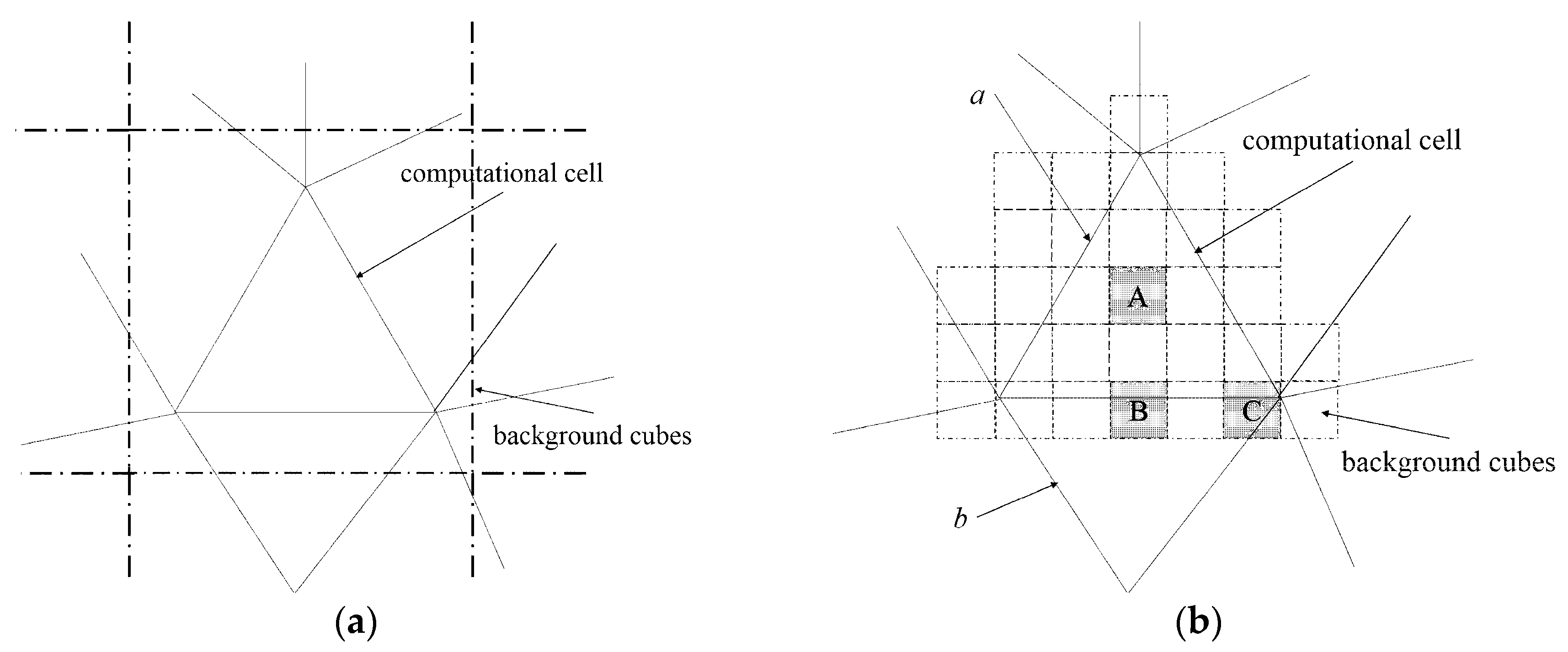
In the existing auxiliary grid methods, the size of the background cube is usually larger than that of the computational cell, as shown in Figure 1a. If a cube overlaps with n (n = 11 in Figure 1a) computational cells, the particle-in-cell tests should be conducted for at least n – 1 (10 in this case) times to find the its host cell. In PLUG method, the background grid adopts a much smaller grid spacing than that of the computational mesh, as shown in Figure 1b. As a result, the cube-to-cell mapping relation is simplified, i.e. the number of the cells related to a given cube is reduced. An internal cube is completely contained by a computational cell, e.g., cube A contained by cell a. For the particles inside an internal cube, the particle-in-cell test is avoided. A boundary cube, which overlaps with the boundary of the computational cell, is related to only a few nearby cells, e.g., cube B is only related to cells a and b. The time-consuming particle-in-cell tests are also reduced.

A resulted side effect with the small-spacing background grid is that it is not easy to derive cube2cell directly. However, an inverse mapping relation can be constructed much more easily, i.e., by finding the background cubes which are fully or partially covered by a certain computational cell. This mapping relation is represented by a list named as cell2cube, with the length being the total number of the computational cell. Each component of this list is still an integer array consisting of the indices of a set of background cubes. For example, considering the computational cell C_J, a set of background cubes is $\left[{\tilde{C}}_{bJ1,}{\tilde{C}}_{bJ2,\dots ,}{\tilde{C}}_{bJt}\right]$, which are the background cubes fully or partially covered by the corresponding computational cell, i.e., satisfying

$$S_{bJq}\cap {\tilde{S}}_J\ne 0\left(q=1 \mathrm{to} t\right),$$

(7)

where ${\tilde{S}}_{bJq}$ is the volume covered by background cube ${\tilde{C}}_{bJq}$ and S_J is the volume covered by computational cell C_J.

The list cube2cell is then obtained by applying an inversion operation of the list cell2cube.

Using the proposed method for the particle locating, the procedure to specify the mapping relation becomes more complicated compared with the existing methods, where a much larger grid spacing is used on background grid. However, in cube2cell list, many small background cubes are related to just one computational cell, i.e., s = 1, and the point-in-cell test is avoided. The overall computational overheads will be greatly reduced, since the procedure to specify the mapping relation is conducted only once for a fixed computational mesh, whereas the point-in-cell test is carried out at every time step and it is a time-consuming operation during the simulation, especially in cases with polyhedral mesh.

The procedures adopted to create lists cell2cube and cube2cell are described as follows.

2.2.1. Creating the Cell2cube List

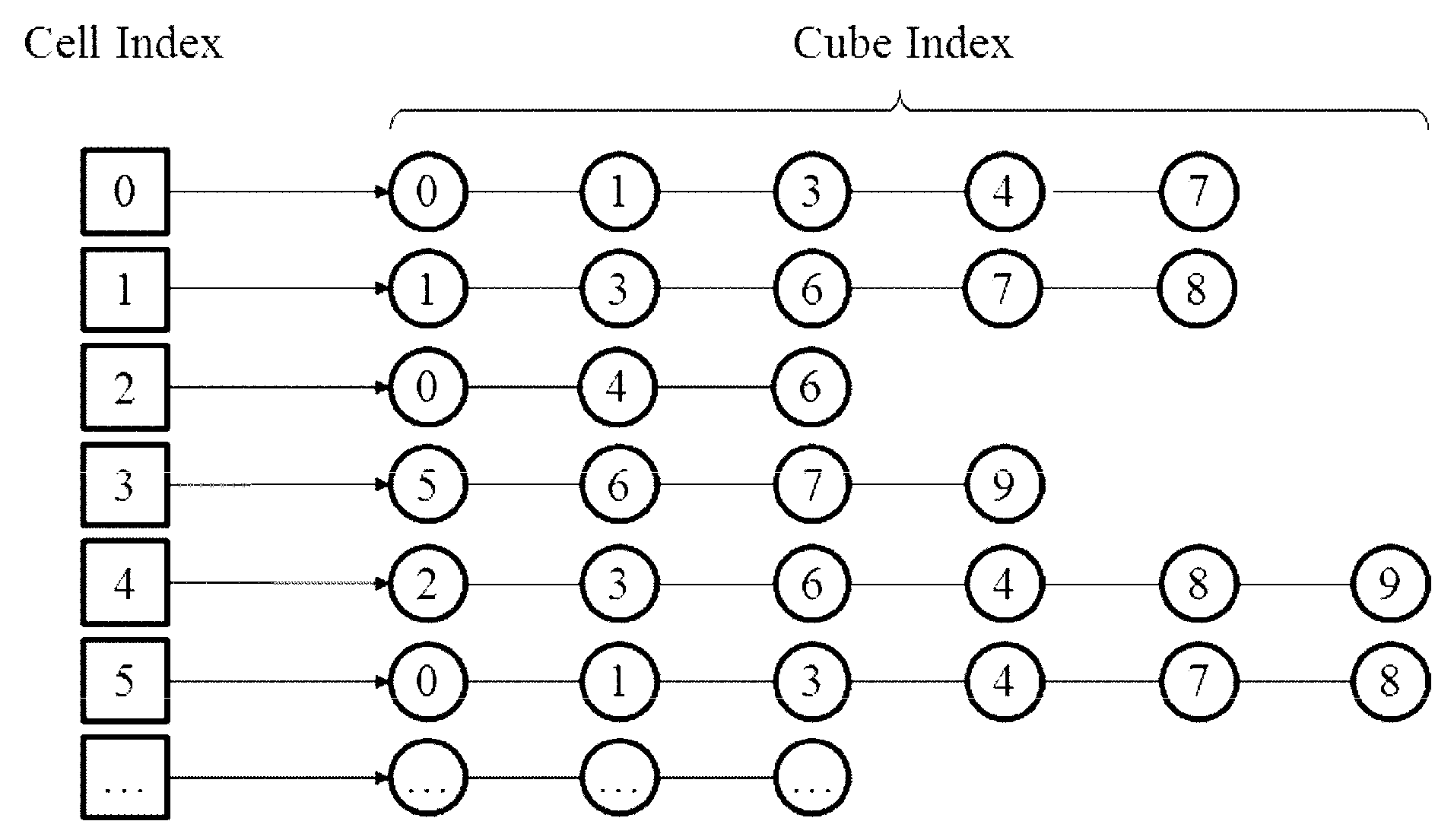
In this part, we describe the procedure to create the cell2cube list. An illustration of a such list is shown in Figure 2.

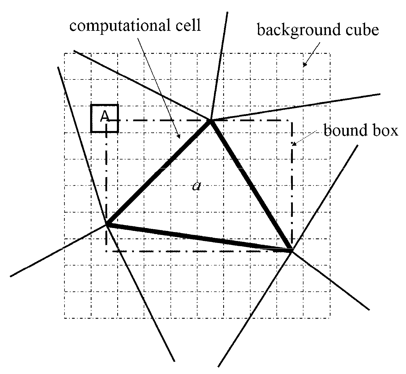
In existing auxiliary grid methods, a minimum cuboid (bound box) encapsulating a computational cell is used to construct the mapping relation. As shown in Figure 3, the bound box of computational cell a is marked in grey. Using the boundary box, the cubes related to a cell are those which intersect with its boundary box. Since the background cubes are much smaller than the computational cells in the present study, boundary box method would introduce many useless cubes. For example, cube A in Figure 3 intersects with the boundary box of cell a, whereas it doesn’t intersect with cell a. To improve the computational efficiency, a new method based on characteristic points is developed in this study.

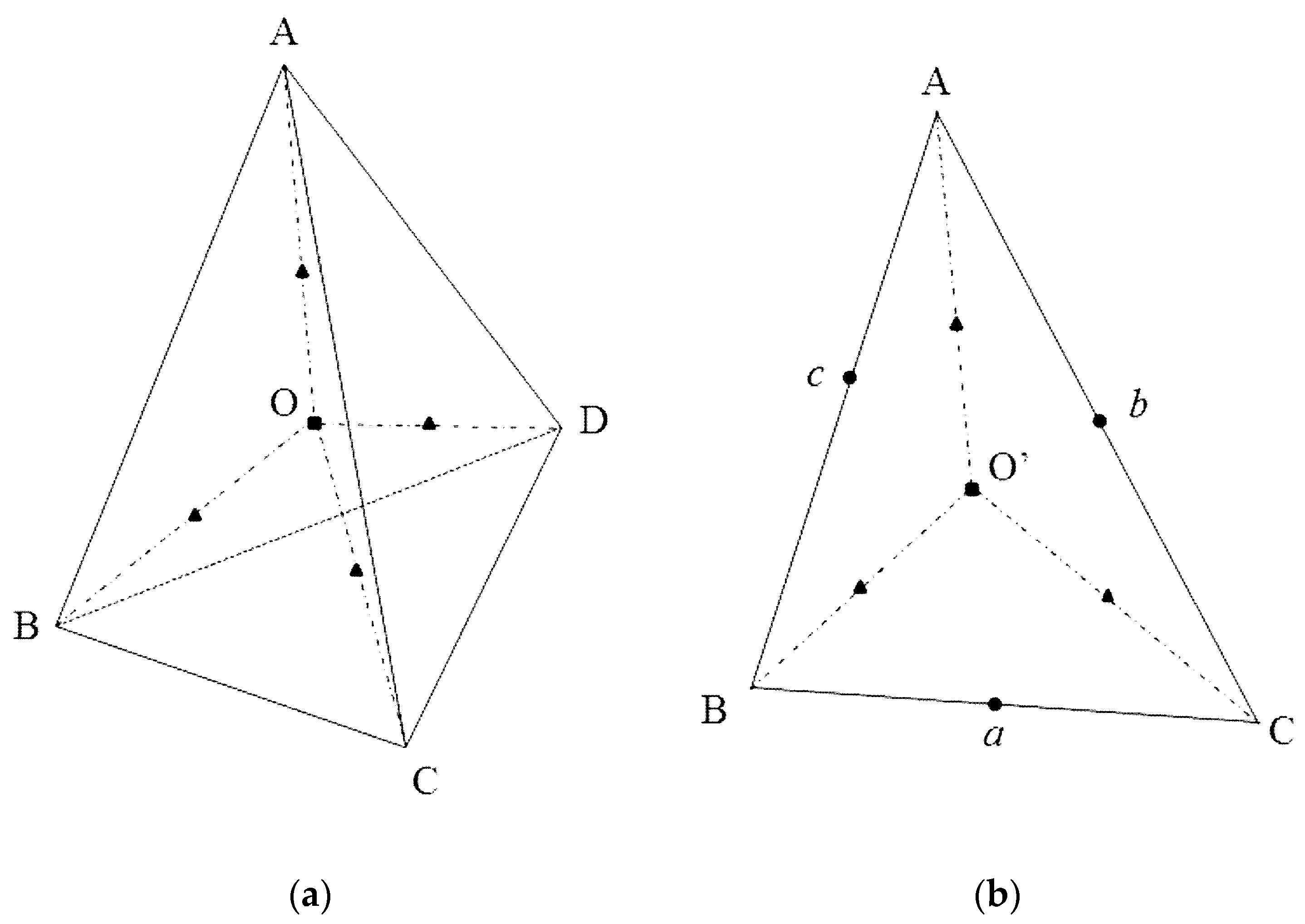
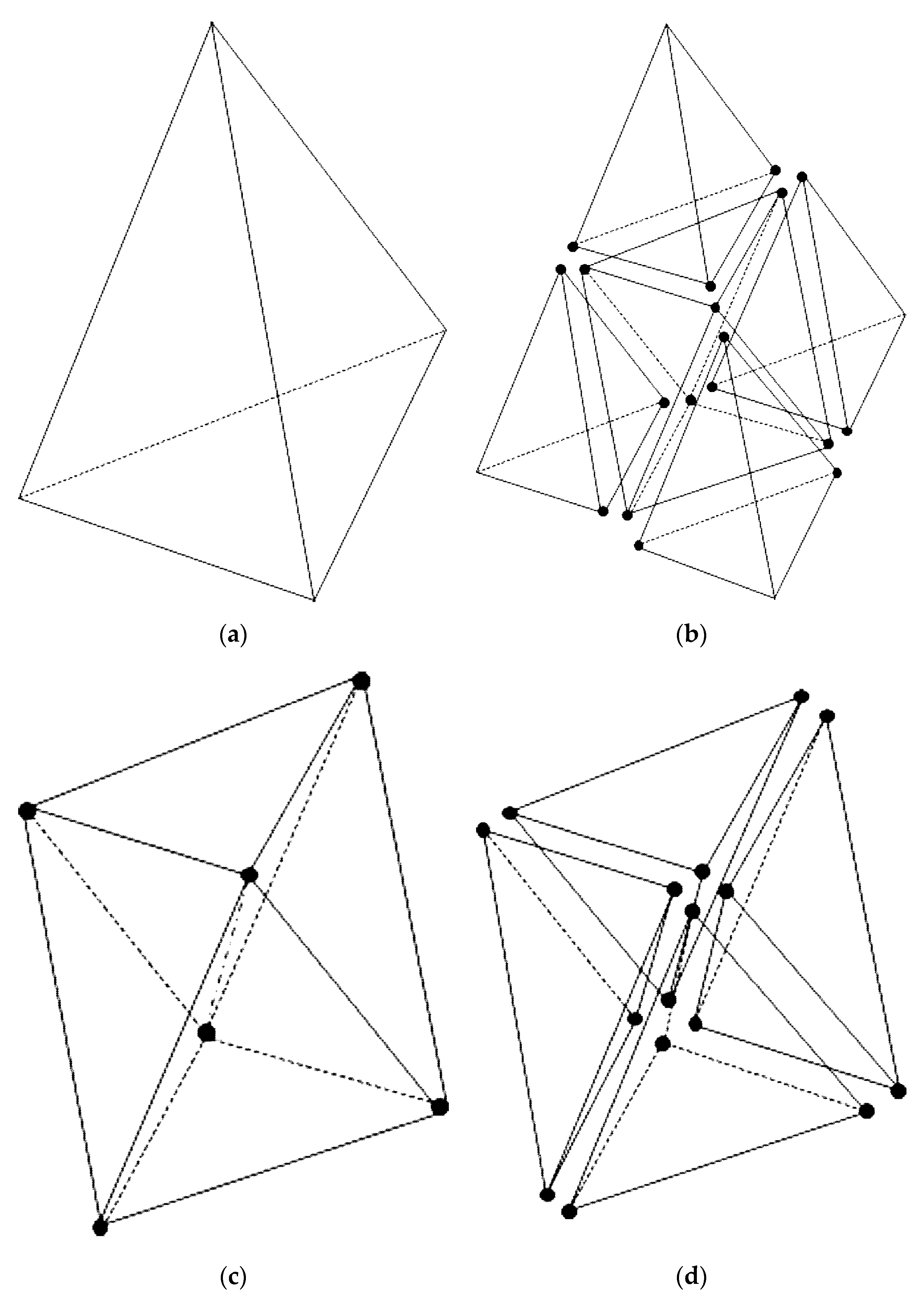
The characteristic point method is developed to check the intersection of a tetrahedron and a cube. We first apply the tetrahedral decomposition on all polyhedral computational cells [15]. Then we use the characteristic point method to find all background cubes which are fully or partially covered by a certain tetrahedron. To create the cell2cube list, each component corresponding to C_J will be a union set of indices of background cubes fully or partially covered by several tetrahedrons decomposed from C_J. Therefore, the procedure described hereafter can be applied on the arbitrary polyhedral mesh. In order to find all the background cubes covered by a given tetrahedron, several characteristic points are defined for the tetrahedron. As shown Figure 4, two types of the characteristic points are adopted in this study, i.e., the interior points shown in panel (a) and the boundary points shown in panel (b). Within each tetrahedron (panel (a) of Figure 4), the characteristic points are the centroid (point O) and the centers of lines $\overline{OA}$, $\overline{OB}$, $\overline{OC}$, and $\overline{OD}$. On each boundary surface (triangle ABC in panel (b) of Figure 2), the characteristic points are the centroid (point $O^{\prime }$), the centers of edges $\overline{AB}$, $\overline{BC}$, and $\overline{CA}$, and the centers of the lines $\overline{O^{\prime }A}$, $\overline{O^{\prime }B}$, and $\overline{O^{\prime }C}$.

In this study, we adopt the background cubes containing the characteristic points and their neighbors as the background cubes fully or partially covered by the tetrahedron. The neighbors of a given background cube are defined as those background cubes that share at least one vertex with it. Apparently, if a tetrahedron is small enough compared with the background cube, the background cubes found using this rule will completely cover this tetrahedron. For a tetrahedron far larger than the background cube, a subdivision will be applied, as shown in Figure 5. Panel (a) shows the original tetrahedron, and panel (b) shows the initial subdivision. The black points in the figure are the centers of the boundary edges. It should be noted that, after initial subdivision, four tetrahedrons and an octahedron are formed. The octahedron is given in panel (c). This octahedron is further decomposed into four tetrahedrons through a line passing through its two opposite vertices, as shown in panel (d). After a subdivision, the above searching scheme will be conducted again to find the background cubes fully or partially covered by the computational cells. For a certain computational cell, searching is completed if no new background cube is found. Otherwise, the subdivision will continue until no new background cube is found to have intersection with corresponding computational cells.

The above process is carried out for each computational cell, and the cell2cube is obtained.

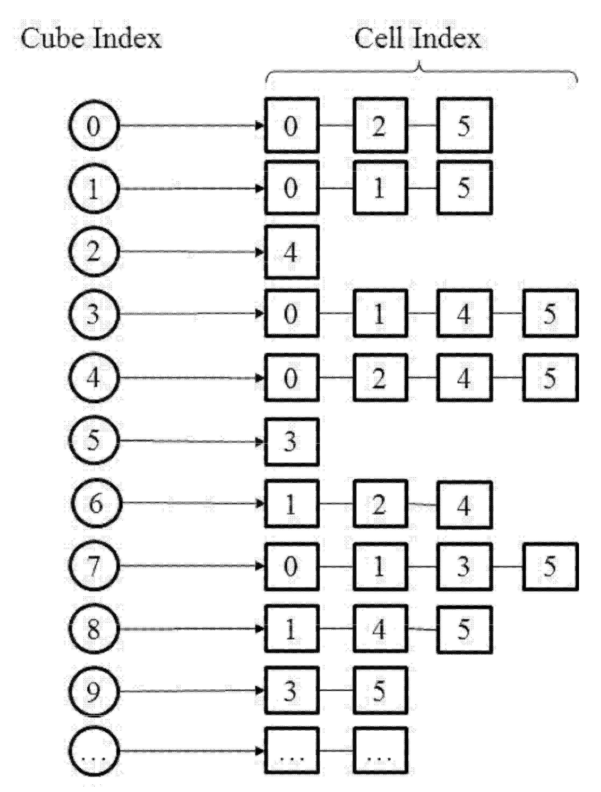
2.2.2. Creating the Cube2cell List

The cube2cell list stores the indices of the computational cells covering a certain background cube. It can be immediately obtained through applying an inverse operation on the cell2cube, constructed in the previous section. Figure 6 gives an illustration of the cube2cell corresponding to the cell2cube list given in Figure 2. By searching the cell2cube list given in Figure 2, one can get that background cube 0 is covered by computational cell 0, 2, and 5, and as a result, the indices of computational cells stored in the first component of the cube2cell list are 0, 2, and 5, as shown in Figure 4. The inverse operation is easily achieved and implemented, and finally the cube2cell list is obtained.

Once the host cell of a certain particle on background grid has been found, the computational cells with their indices stored in corresponding component of the list cube2cell will be checked to finally determine the host cell.

2.3. Particle Locating

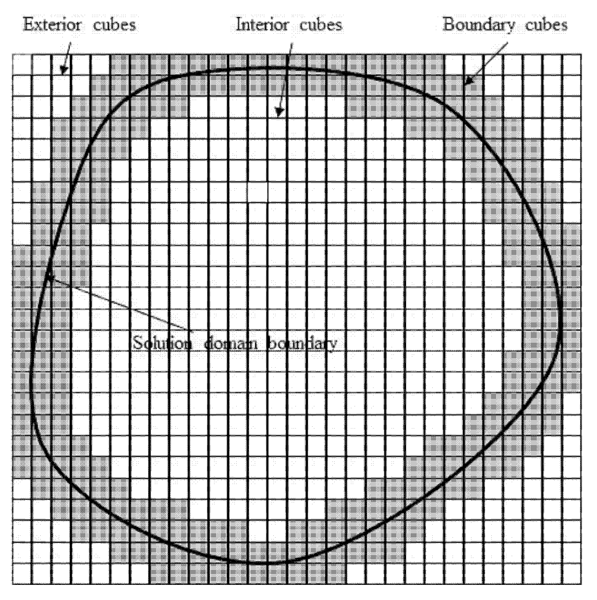
PLUG uses different procedures to find the host cell for a given particle within different types of host background cubes. In PLUG, background cubes are categorized into three different types (as shown in Figure 7).

• Exterior cubes. There are some background cubes which are not covered by any computational cell, since the physical domain covered by background grid is a little larger than the computational domain, as we have mentioned in Section 2.1. In this case, the corresponding component in the cube2cell list is empty.
• Boundary cubes. The boundary elements are the cubes near the boundary surface of the computational domain. One can find the background cubes for a given polygonal face on boundary with the same method as that for finding those for a given computational cell. A general polygon is decomposed into several triangles. The characteristic points for searching are shown in Figure 4b, and the subdivision process for a triangle is the same as that for the boundary surface of a tetrahedron, as shown in Figure 5b.
• Interior cubes. All the elements, excluding exterior cubes and boundary cubes belong to this type.

Similar to the cube2cell list, the element types are decided just once before the simulation with a fixed computational mesh.

In order to find the host cell for a given particle, the host cells on background grid are determined using (3). If the indices satisfy $i\in \left[0,n_x-1\right]$, $j\in \left[0,n_y-1\right]$ and $k\in \left[0,n_z-1\right]$, the point is inside the domain of the background grid. Otherwise, the point is outside the background grid, and it will not be inside any cell of the computational mesh. For the point inside the background grid, three situations are considered, corresponding to the type of the host background cell as

• For particles inside an exterior cube, these particles are outside the computational domain and not in any polyhedral computational cell.
• For particles inside a boundary cube, the point-in-cell test is adopted to check whether these points are inside one of the computational cells stored in the corresponding component of the cube2cell list. If a computational cell is found, it is the host cell. Otherwise, this particle is out of the computational domain.
• For particles inside an interior cube, the point-in-cell test is carried out to find the host cell. It is worth nothing that, in this case, some background cubes are contained by only one computational cell, and only one index appears in the corresponding component of the cube2cell list. In this case, the host cell can be determined without any point-in-cell test. This makes the PLUG method much more efficient than existing point locating algorithms.

For those problems where particles are always inside the solution domain, there is no need to distinguish the types of the background cubes. However, for an open system, though there is only one index stored in some components of the cube2cell list, the corresponding computational cell may not be the host cell. If the background cube is a boundary cube, the particle may be out of the computational domain.

So far, the remaining task is to check whether a point is inside a polyhedral cell or not, i.e., the point-in-cell test. We first carry out a plane testing for each boundary surface of the computational cell as

$$l=\mathbf{n}\cdot \left(x_p-x_c\right)$$

(8)

where n is the outward normal direction of a boundary surface, x_p is the location of the tested point, and x_c is the location of centroid of the surface.

Equation (8) is tested for all boundary surfaces of a computational cell. If l > 0 for some surface, the point will be outside the cell, otherwise, it is inside the cell. If the boundary surface is triangle, the above test can be applied directly. With a polygon other than triangle, an efficient and reliable solution is to decompose all the polygonal surfaces into triangles using vertex-based method or center-based method at first [15], and then conducting testing in (8).

3. Tests and Results

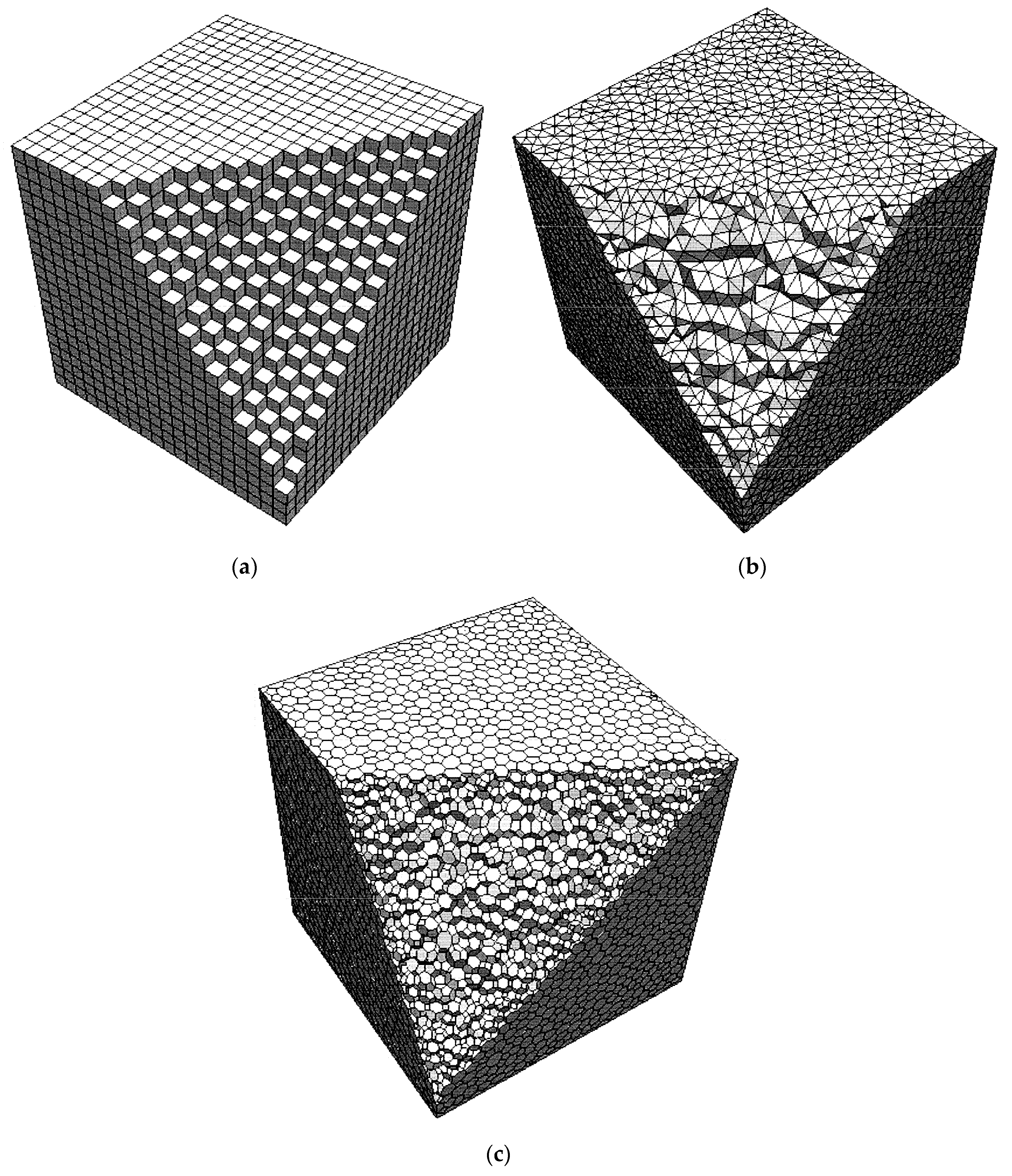
Three different types of meshes shown in Figure 8 were adopted to test the efficiency of the proposed PLUG method. All these meshes were generated for a cubic domain of 1 m × 1 m × 1 m. In Figure 8, a part of the mesh is cut out to show the mesh cells inside. The hexahedral mesh shown in Figure 8a includes 14,400 cells. The tetrahedral mesh, shown in Figure 8b, generated through Delaunay method, includes 14,333 tetrahedral cells. The polyhedral mesh, shown in Figure 8c, includes 14,645 polyhedral cells. The particles for tests were generated using the following method

$${\mathrm{x}}_p={\mathrm{x}}_{cJ}+0.5V_J^{\frac{1}{3}}\left[\mathrm{rand}\left(-1,1\right),\mathrm{rand}\left(-1,1\right),\mathrm{rand}\left(-1,1\right)\right]$$

(9)

where, ${\mathrm{x}}_p$ is the location of the generated point, J is the index of a randomly selected cell, ${\mathrm{x}}_{cJ}$ and V_J are the location of the center and the volume of the cell. Function rand (−1, 1) returns random real number in the range of [−1, 1].

In this study, the binary search method (denoted by octree) and the face-to-face method [6] (denoted by GNH) were adopted, to compare with the proposed PLUG method. The GNH method was conducted with different choices of the starting point, and resulted algorithms are denoted by GNH, GNHNC, and GNHHC. In GNH, the starting point is always located at the center of cell 0. In GNHNC, the starting point for each particle is the center of one of neighbor cells of its host cell. In GNHHC, the starting point is the center of the host cell of each particle. As a result, the operations in GNHNC for each particle are point-in-cell test in starting host cell at first, followed by finding the nearest neighbor cell, which is the correct host cell, and finally the point-in-cell test in the correct host cell. In GNHHC, only the point-in-cell test is conducted, once for each particle, to find the host cell which is exactly the starting host cell. Actually, for a practical computation, the starting point is usually chosen as the center of the host cell at the last time step. GNH, GNHNC, and GNHHC are idealized situations corresponding to worst, near optimal, and optimal choices of the starting point, respectively.

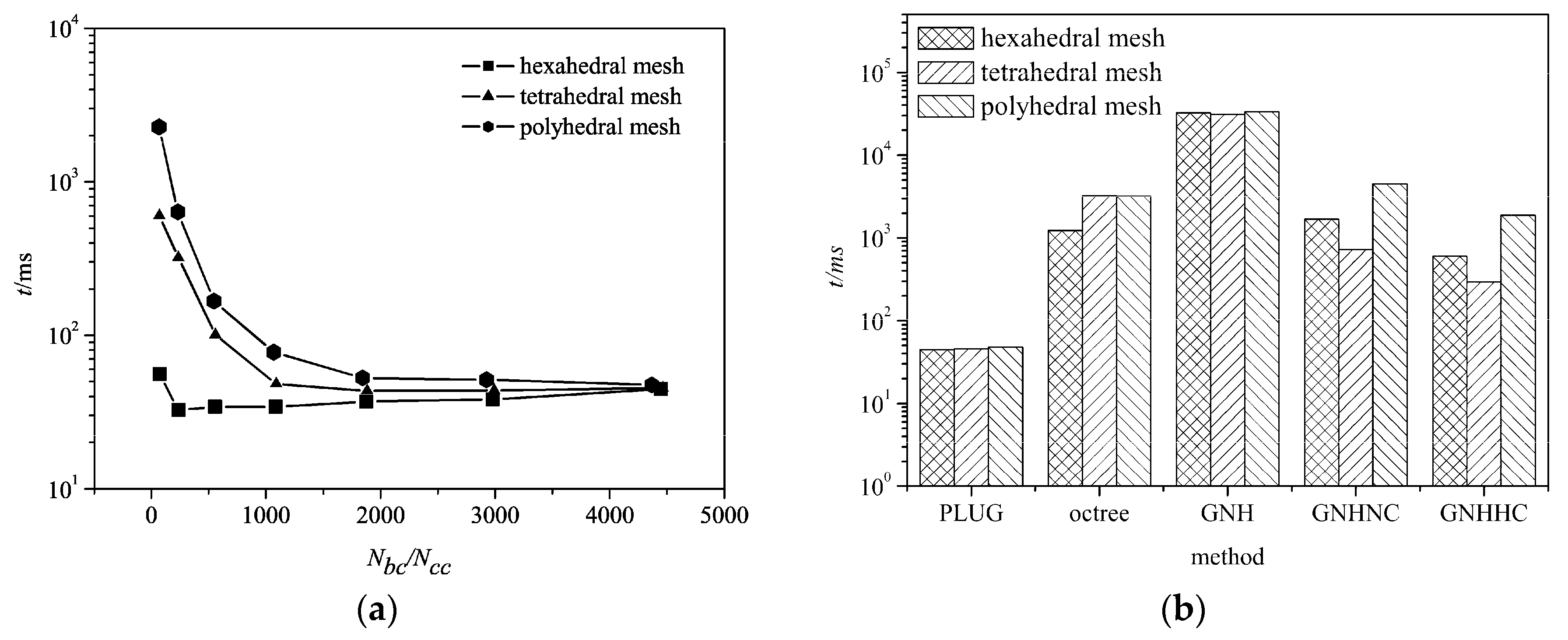
Figure 9 shows CPU times consumed by different methods on three different types of meshes, for locating 1 × 10⁶ particles at randomly selected locations in the computational domain. The computational efficiency of the proposed PLUG method depends on the resolution of the background grid on tetrahedral and polyhedral meshes. Figure 9a shows the change of the CPU times with the ratio of the total number of cubes on background grid (N_bc) and the computational cells (N_cc). When N_bc/N_cc < 1000, the computational efficiency was significantly improved by refining background grids. However, it was unworthy of further increasing the resolution of the background grid after that point, because the CPU time decreased little in the cases with the polyhedral mesh and tetrahedral mesh and increased in the case with hexahedral mesh. Moreover, more memory is required to store the cube2cell list. On the hexahedral grid, the CPU time was almost independent of the resolution of the background grid because of the same topological structure on the background grid and computational meshes. Comparing the CPU times consumed on the different meshes, particle locating was fastest on the hexahedral meshes, followed by the tetrahedral mesh, which was a little faster than the polyhedral mesh. With the refining background grid resolution, the CPU times finally arrived at the same values with a very fine background grid on different meshes.

The CPU times consumed by GNH, GNHNC, GNHHC, and octree methods on different meshes are shown in Figure 9b. GNH method was lowest. By choosing a much better initial guess of the host cell in GHNNC and GNHHC, the computational efficiency was obviously improved. Thus, the computational efficiency of face-to-face methods relies heavily on the starting host cell. With GNHHC method, only the point-in-cell test was conducted. The computational efficiency of the point-in-cell test depended on the types of the computational cell, i.e., fastest on tetrahedral mesh and slowest on the polyhedral mesh. The reason is that cells with more boundary faces require more CPU time to conduct the operation defined in (8). Octree method had similar computational overheads to the GNHNC methods. The PLUG algorithm (with 400³ background cubes) was the fastest one among all methods and its computational efficiency was independent of the types of the computational cells.

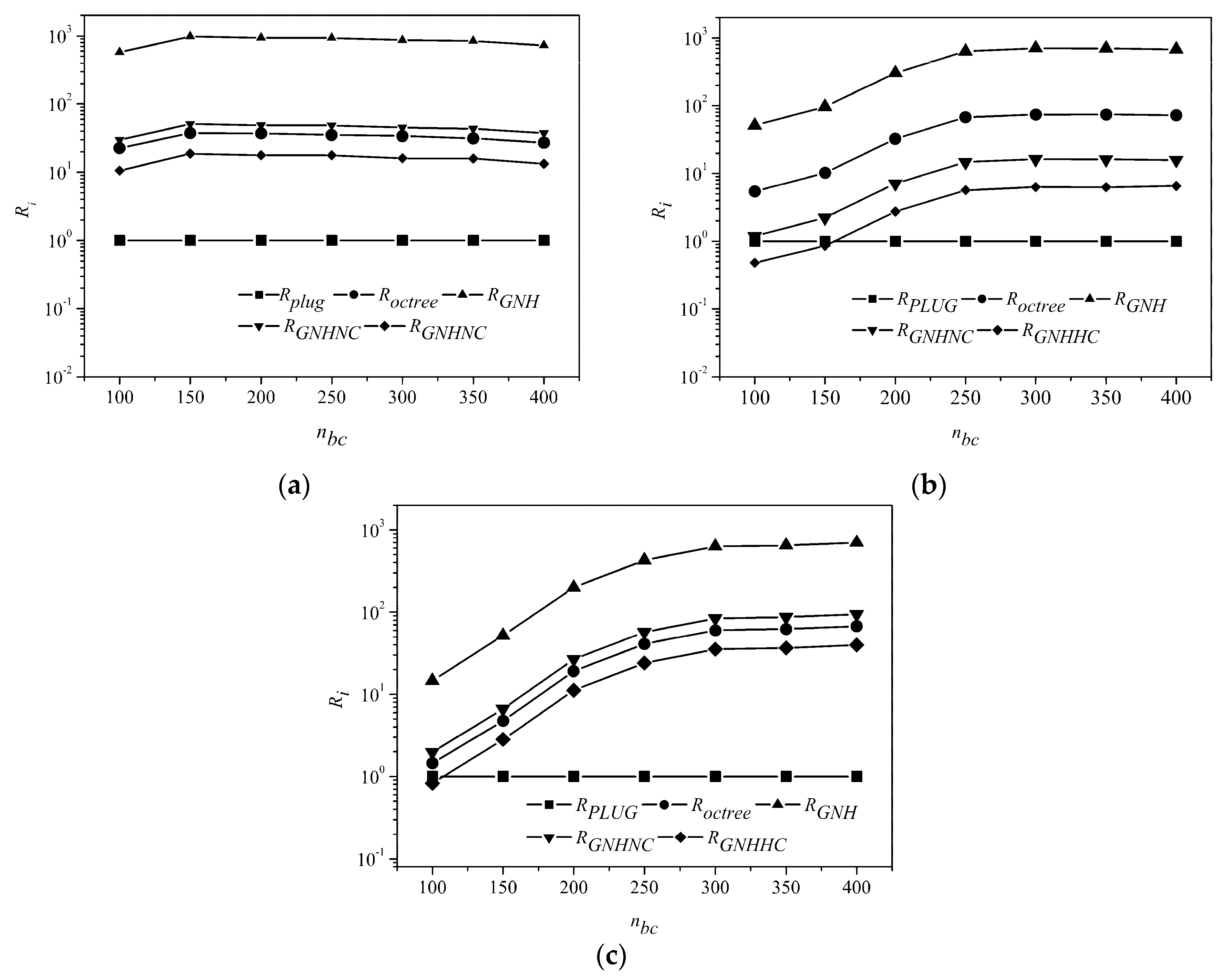
Shown in Figure 10 is the relative CPU times of octree, GNH, GNHNC, GNHHC methods normalized by those of the PLUG method, with background grid of different resolutions. The horizontal axis is the number of background cubes in one spatial direction. The total number of background cubes is $N_{bc}=n_{bc}^3$. The PLUG method was better than octree and GNH methods on all three meshes with any background grids. On the hexahedral mesh, the PLUG method was always the best one, which was about 17.8 times, 50.2 times, 984.9 times, 36.5 times faster than GNHHC, GNHNC, GNH, and octree methods. With a coarse 100³ background grid, CPU time consumed by PLUG method was about two times that of GNHHC and similar to that of GNHNC on the tetrahedral mesh. As the CPU times of PLUG method reduced very quickly with the increasing resolution of the background grid, the CPU time of the PLUG method was about 15% of that of the GNHRC method and 6.3% of that of the GNHNC, using a 400³ background grid on the tetrahedral mesh. Similar results were observed on the polyhedral mesh. The PLUG method had the similar computational overheads to the GNHHC method and a little larger expenses than that of the GNHHC method, when using 100³ background grid. Increasing the number of the background cubes to 400³, the PLUG method was about 38.7 times faster than the GNHHC method.

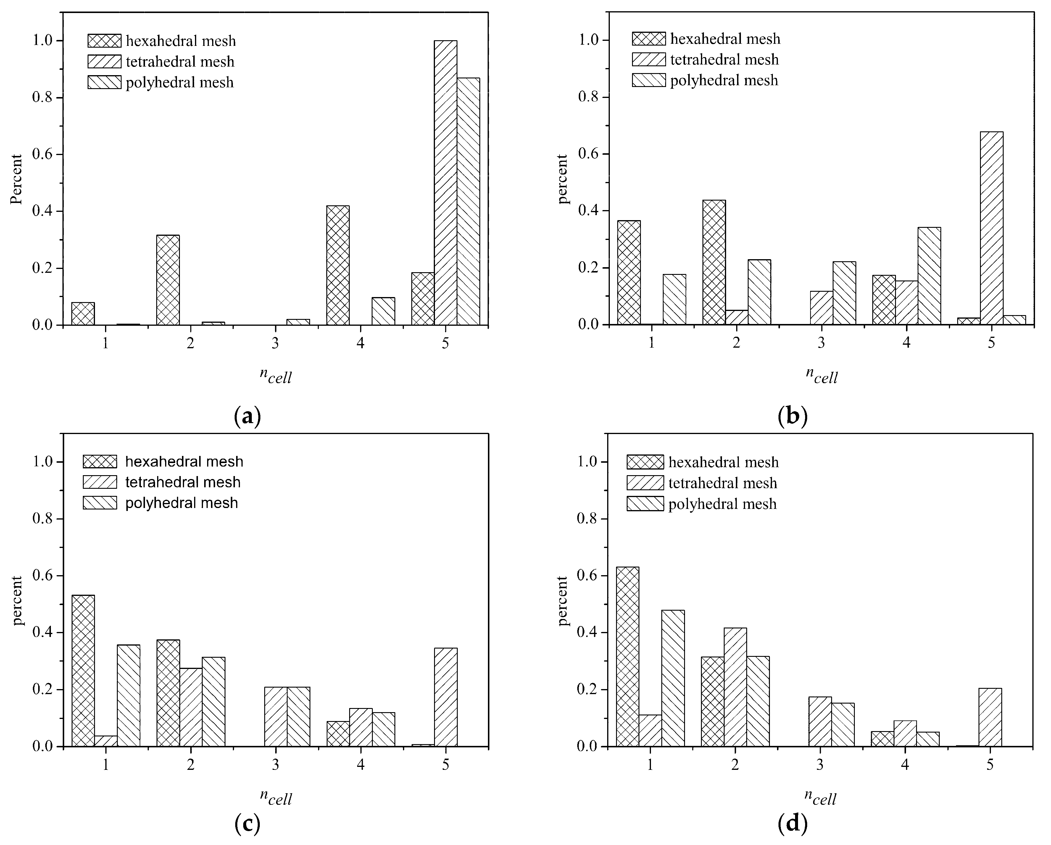
The proposed PLUG method is faster than GHNHC and independent of the types of meshes if a background grid with adequate cubes is adopted. As the method GNHHC has an optimal starting host cell and only one point-in-cell test is required, the reason for better computational efficiency of the PLUG method is that the point-in-cell test is not conducted for many particles during searching their host cells. In other words, there are many background cubes that are fully contained by a computational cell, since the background cubes are much smaller than computational cells on fine background grid. For clarifying this point of view, we conducted a count of the number of such background cubes during the numerical tests, and the results are shown in Figure 11. The horizontal axis is the given number of the computational cells. The vertical axis is the percentage of the cubes covered by a given number of cells. It should be pointed out that the percentage corresponding to number 5 means the percentage of the background cubes covered by more than four computational cells. The computational efficiency of the PLUG method can be explained by the percentages corresponding to the number 1 and 5 in Figure 11. It can be seen that, with a 100³ background grid, the percentage of the background cubes covered by more than four cells was about 18.5%, 99.99%, and 86.9% on the hexahedral mesh, tetrahedral mesh, and the polyhedral mesh, respectively. As a result, the CPU times consumed by the PLUG method on tetrahedral and polyhedral grid were much larger than that on the hexahedral mesh. With the increasing resolution of the background grid, the percentage of the cubes covered by more than four cells reduced on all meshes. With a 400³ background grid, the percentage reduced to 20.47% on the tetrahedral mesh and 0.00058% on the polyhedral mesh. The computational efficiency was then highly improved. The percentage of the cubes covered by one computational cell increased on all three meshes with refined background grids. However, it increased much faster on the tetrahedral meshes and the polyhedral meshes than on the hexahedral mesh. As a result, the PLUG method was much more sensitive to the background grid resolution on the tetrahedral and polyhedral meshes, as shown in Figure 9.

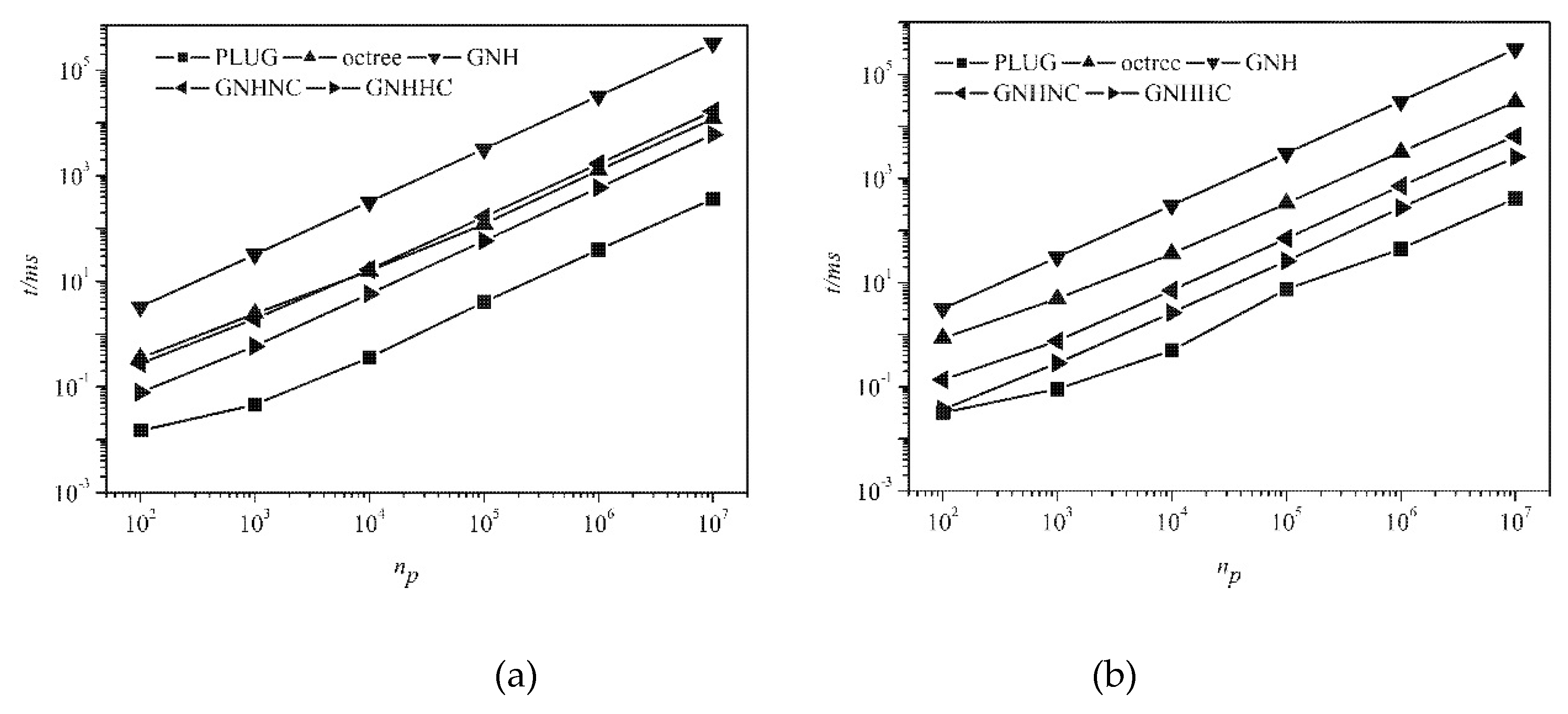
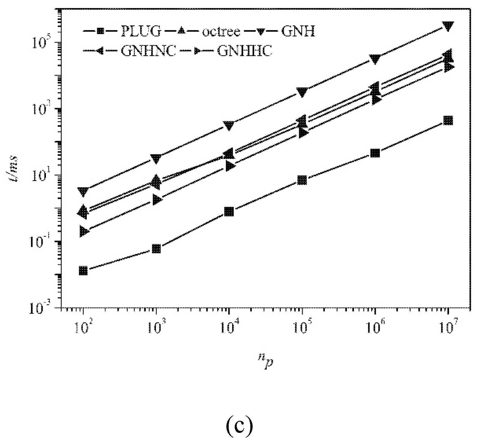
Scalability analysis was conducted by checking the CPU time consumed by different methods for locating the gradually increasing number of particles in the computational domain, which is of essential importance to judge whether a particle locating algorithm can be used in a practical application. The evolution of CPU time with the increasing number of particles is shown in Figure 12 for different meshes. The background grid used by the PLUG method adopted 400³ cubes. The PLUG method was the best one of all adopted locating methods in all tests. And all methods had the similar time complexity.

4. Summary

In this work, a new, efficient, and robust method, namely PLUG, for particle locating is proposed. Using the PLUG method, the auxiliary grid method is extended to three-dimensional arbitrary polyhedral mesh. A uniform Cartesian grid is adopted as the background grid. By choosing a much smaller grid spacing for the background grid compared with that of the computational mesh, the PLUG method is highly efficient compared with the existing methods (GNH, GNHNC, GNHHC, and octree). For the particles belonging to the background cubes which are covered by only one computational cell, it is not necessary to conduct the point-in-cell test. With the fine background grid, the percentage of such background cubes becomes high. This is the main reason for the high computational efficiency of the PLUG method relative to the existing methods. Numerical tests were carried out for particle locating of the random distributed particles on three different types of computational meshes, i.e., hexahedral mesh, tetrahedral mesh, and polyhedral mesh. The results revealed that

(1) PLUG is much more efficient than the face-to-face searching method (GNH, GNHNC, GNHHC) and the octree method on all three types of mesh with a relatively fine background grid. The computational expense of the Octree method is the largest. For face-to-face searching methods, the computational expense of GNH is the largest, GNHHC is the smallest, and GNHNC is between GNH and GNHHC, depending on the distance between the starting point and the host cell.

(2) The efficiency of PLUG is relevant to the configuration of the background grid on the tetrahedral and the polyhedral meshes. The background grid with finer resolution results in a higher computational efficiency. On hexahedral mesh, PLUG is not sensitive to the resolution of the background grid due to its same topological structure with the background grid.

References

- Su, J.; Gu, Z.; Xu, X.Y. Discrete element simulation of particle flow in arbitrarily complex geometries. Chem. Eng. Sci. 2011, 66, 6069–6088. [Google Scholar] [CrossRef]
- Su, J.; Gu, Z.; Zhang, M.; Xu, X.Y. An improved version of RIGID for discrete element simulation of particle flows with arbitrarily complex geometries. Powder. Techno. 2014, 253, 393–405. [Google Scholar] [CrossRef]
- Chen, X.Q.; Pereira, J.C.F. A new particle-locating method accounting for source distribution and particle-field interpolation for hybrid modeling of strongly coupled two-phase flows in arbitrary coordinates. Numer. Heart Transf. B 1991, 35, 41–63. [Google Scholar]
- Vaidya, A.M.; Subbarao, P.M.V.; Gaur, R.R. A Novel and Efficient Method for Particle Locating and Advancing over Deforming, NonOrthogonal Mesh. Numer. Hear. Tran. B. 2006, 49, 67–88. [Google Scholar] [CrossRef]
- Haselbacher, A.; Najjar, F.M.; Ferry, J.P. An efficient and robust particle- localization algorithm for unstructured grids. J. Comput. Phys. 2007, 225, 2198–2213. [Google Scholar] [CrossRef]
- Martin, G.D.; Loth, E.; Lankford, D. Particle host cell determination in un- structured grids. Comput. Fluids 2009, 38, 101–110. [Google Scholar] [CrossRef]
- Ke, P.; Zhang, S.; Wu, J.; Yang, C. An improved known vicinity algorithm based on geometry test for particle localization in arbitrary grid. J. Comput. Phys. 2009, 228, 9001–9019. [Google Scholar] [CrossRef]
- Capodaglio, G.; Aulisa, E. A particle tracking algorithm for parallel finite element applications. Comput. Fluids 2017, 159, 338–355. [Google Scholar] [CrossRef]
- Stuart, D.C.C.; Kleijn, C.R.; Kenjereš, S. An efficient and robust method for Lagrangian magnetic particle tracking in fluid flow simulations on unstructured grids. Comput. Fluid. 2011, 40, 188–194. [Google Scholar] [CrossRef]
- Seldner, D.; Westermann, T. Algorithms for interpolation and localization in irregular 2D meshes. J. Comput. Phys. 1988, 79, 1–11. [Google Scholar] [CrossRef]
- Muradoglu, M.; Kayaalp, A.D. An auxiliary grid method for computations of multiphase flows in complex geometries. J. Comput. Phys. 2006, 214, 858–877. [Google Scholar] [CrossRef]
- Macpherson, G.B.; Nordin, N.; Weller, H.G. Particle tracking in unstructured, arbitrary polyhedral meshes for use in CFD and molecular dynamics. Comm. Numer. Meth. Eng. 2010, 25, 263–273. [Google Scholar] [CrossRef]
- Jin, H.; He, C.; Chen, S.; Wang, C.; Fan, J. A method of tracing particles in irregular unstructured grid system. J. Comput. Multiph. Flows. 2013, 5, 231–238. [Google Scholar] [CrossRef]
- Sani, M.; Saidi, M.S. A set of particle locating algorithms not requiring face belonging to cell connectivity data. J. Comput. Phys. 2009, 228, 7357–7367. [Google Scholar] [CrossRef]
- Ferziger, J.H.; Peric, M. Computational Methods for Fluid Dynamics, 3rd ed.; Springer: Berlin, Germany, 2012. [Google Scholar]
Figure 1.
An illustration of different background grid configurations. (a) large-spacing grid; (b)small-spacing grid.
Figure 2.
An illustration of the cell2cube list.
Figure 3.
Overlap relation determination in existing auxiliary grid method.
Figure 4.
Characteristic points for a tetrahedrom. (a) Interior points; (b) Boundary points.
Figure 5.
The sub-division of a tetrahedron. (a) Original tetrahedron; (b) Initial subdivision; (c) Central octahedron; (d) Subdivision of central octahedron.
Figure 6.
An illustration of a cube2cell list.
Figure 7.
Different types of the background cubes.
Figure 8.
Three different types of meshes used in numerical tests. (a) Hexahedral mesh; (b) Tetrahedral mesh; (c) Polyhedral mesh.
Figure 9.
CPU times consumed by different particle-locating methods on different grids. (a) CPU times of PLUG method; (b) CPU times of other methods.
Figure 10.
Normalized CPU times. (a) Hexahedral mesh; (b) Tetrahedral mesh; (c) Polyhedral mesh.
Figure 11.
The percentage of background cubes covered by a given number of computational cells. (a) Background grid with 1003 cells; (b) Background grid with 2003 cells; (c) Background grid with 3003 cells; (d) Background grid with 4003 cells.
Figure 12.
Scalability of the different methods with regard to the increasing number of the particles on the different types of meshes. (a)Hexahedral mesh; (b) Tetrahedral mesh; (c) Polyhedral mesh.
© 2019 by the authors. Licensee MDPI, Basel, Switzerland. This article is an open access article distributed under the terms and conditions of the Creative Commons Attribution (CC BY) license (http://creativecommons.org/licenses/by/4.0/).
Share and Cite
MDPI and ACS Style
Li, Z.; Wang, Y.; Wang, L. A Fast Particle-Locating Method for the Arbitrary Polyhedral Mesh. Algorithms 2019, 12, 179. https://0-doi-org.brum.beds.ac.uk/10.3390/a12090179
AMA Style
Li Z, Wang Y, Wang L. A Fast Particle-Locating Method for the Arbitrary Polyhedral Mesh. Algorithms. 2019; 12(9):179. https://0-doi-org.brum.beds.ac.uk/10.3390/a12090179
Chicago/Turabian StyleLi, Zongyang, Yefei Wang, and Le Wang. 2019. "A Fast Particle-Locating Method for the Arbitrary Polyhedral Mesh" Algorithms 12, no. 9: 179. https://0-doi-org.brum.beds.ac.uk/10.3390/a12090179
Note that from the first issue of 2016, this journal uses article numbers instead of page numbers. See further details here.