A FEAST Algorithm for the Linear Response Eigenvalue Problem


1
College of Computer and Information Science, Fujian Agriculture and Forestry University, Fuzhou 350002, China
2
School of Mathematical Sciences, Guizhou Normal University, Guiyang 550001, China
*
Author to whom correspondence should be addressed.
Algorithms 2019, 12(9), 181; https://0-doi-org.brum.beds.ac.uk/10.3390/a12090181
Submission received: 22 July 2019
/
Revised: 25 August 2019
/
Accepted: 27 August 2019
/
Published: 29 August 2019
Abstract
:In the linear response eigenvalue problem arising from quantum chemistry and physics, one needs to compute several positive eigenvalues together with the corresponding eigenvectors. For such a task, in this paper, we present a FEAST algorithm based on complex contour integration for the linear response eigenvalue problem. By simply dividing the spectrum into a collection of disjoint regions, the algorithm is able to parallelize the process of solving the linear response eigenvalue problem. The associated convergence results are established to reveal the accuracy of the approximated eigenspace. Numerical examples are presented to demonstrate the effectiveness of our proposed algorithm.
1. Introduction
In computational quantum chemistry and physics, the random phase approximation (RPA) or the Bethe–Salpeter (BS) equation describe the excitation states and absorption spectra for molecules or the surfaces of solids [1,2]. One important question in the RPA or BS equation is how to compute a few eigenpairs associated with several of the smallest positive eigenvalues of the following eigenvalue problem:
where are both symmetric matrices and is positive definite [3,4,5]. Through a similarity transformation, the eigenvalue problem (1) can be equivalently transformed into:
where and . The eigenvalue problem (2) was still referred to as the linear response eigenvalue problem (LREP) [3,6] and will be so in this paper, as well. The condition imposed upon A and B in (1) implies that both K and M are real symmetric positive definite matrices. However, there are cases where one of them may be indefinite [7]. Therefore, to be consistence with [8,9,10], throughout the rest of the paper, we relax the condition on K and M to that they are symmetric and one of them is positive definite, while the other may be indefinite. There has been immense recent interest in developing new theories, efficient numerical algorithms of LREP, and the associated excitation response calculations of molecules for materials’ design in energy science [11,12,13,14,15].
From (2), we have and , and they together lead to:
Since has the same eigenvalues as , which is symmetric, all eigenvalues of are real. Denote these eigenvalues by () in ascending order, i.e.,
The eigenvalues of are (), as well. Let , the imaginary unit, and:
The eigenvalues of H are:
This practice of enumerating the eigenvalues of H will be used later for the much smaller projection of H, as well.
Since the dimension N is usually very large for systems of practical interest, solving LREP (2) is a very challenging problem. The iterative methods are recent efforts for computing the partial spectrum of (2), such as the locally-optimal block preconditioned 4D conjugate gradient method (LOBP4DCG) [6] and its space-extended variation [16], the block Chebyshev–Davidson method [10], as well as the generalized Lanczos-type methods [8,9]. These algorithms are all based on the so-called pair of deflating subspaces, which is a generalization of the concept of the invariant subspace in the standard eigenvalue problems. Thus, these methods can be regarded as extensions of the associated classical methods for the standard eigenvalue problem. Recently, in [17], a density-matrix-based algorithm, called FEAST, was proposed by Polizzi for the calculation of a segment of eigenvalues and their associated eigenvectors of a real symmetric or Hermitian matrix. The algorithm promises high potential for parallelism by dividing the spectrum of a matrix into an arbitrary number of nonintersecting intervals. The eigenvalues in each interval and the associated eigenvectors can be solved independently of those in the other intervals. As a result, one can compute a large number of eigenpairs at once on modern computing architectures, while typical Krylov- or Davidson-type solvers fail in this respect because they require orthogonalization of any new basis vector with respect to the previously-converged ones.
The basic idea of the FEAST algorithm is based on the contour integral function:
to construct bases of particular subspaces and obtain the corresponding approximate eigenpairs by the Rayleigh–Ritz procedure where is any contour enclosing the set of wanted eigenvalues. The corresponding theoretical analysis was established in [18]. In particular, it was shown that the FEAST algorithm can be understood as an accelerated subspace iteration algorithm. Due to the advantage of the FEAST algorithm in parallelism, it has been well received in the electronic structure calculations community. Additionally, the improvements and generalizations of FEAST algorithm have been active research subjects in eigenvalue problems for nearly a decade. For example, in [19], Kestyn, Polizzi, and Tang presented the FEAST eigensolver for non-Hermitian problems by using the dual subspaces for computing the left and right eigenvectors. In [20], the FEAST algorithm was developed to solve nonlinear eigenvalue problems for eigenvalues that lie in a user-defined region. Some other work for the FEAST method can be found in [21,22,23,24]. Motivated by these facts, in this paper, we will continue the effort by extending the FEAST algorithm to LREP.
The rest of the paper is organized as follows. In Section 2, some notations and preliminaries including the canonical angles of two subspaces and basic results for LREP are collected for use later. Section 3 contains our main algorithm, the implementation issue, and the corresponding convergence analysis. In Section 4, we present some numerical examples to show the numerical behavior of our algorithm. Finally, conclusions are drawn in Section 5.
2. Preliminaries
is the set of all real matrices. For , is the dimension of . For , is its transpose and the column space of X, and the submatrix of X consists of column i to column j. is the identity matrix or simply I if its dimension is clear from the context. For matrices or scalars , denotes the block diagonal matrix with diagonal block .
For any given symmetric and positive definite matrix , the W-inner product and its induced W-norm are defined by:
If , then we say or . The projector is said to the W-orthogonal projector onto if for any vector ,
For two subspaces with , let X and Y be the W-orthonormal basis matrices of subspaces and , respectively, i.e.,
Denote the singular values of by for in ascending order, i.e., . The diagonal matrix of W-canonical angles from (If , we may say that these angles are between and [25].) to in descending order is defined by:
where and:
In what follows, we sometimes place a vector or matrix in one or both arguments of with the understanding that it is about the subspace spanned by the vector or the columns of the matrix argument.
Several theoretical properties of the canonical angle and LREP have been established in [25] and [3], respectively. In particular, the following lemmas are necessary for our later developments.
Lemma 1
([9] Lemma 3.2). Let and be two subspaces in with equal dimension . Suppose . Then, for any set of the basis vectors in where , there is a set of linear independent vectors in such that for , where is the W-orthogonal projector onto .
Lemma 2
([3] Theorem 2.3). The following statements hold for any symmetric matrices with M being positive definite.
- (a)
- There exists a nonsingular such that:where , and .
- (b)
- If K is also definite, then all , and H is diagonalizable:
- (c)
- The eigen-decomposition of and is:respectively.
Lemma 3
([10] Lemma 2.2). Let be an invariant subspace of H and be the basis matrix of with both V and U having N rows, then .
Lemma 4
([25] Lemma 2.1). Let A and B be two symmetric matrices and and be the set of the eigenvalues of A and B, respectively. For the Sylvester equation , if , then the equation has a unique solution Y, and moreover:
where over all and .
3. The FEAST Algorithm for LREP
3.1. The Main Algorithm
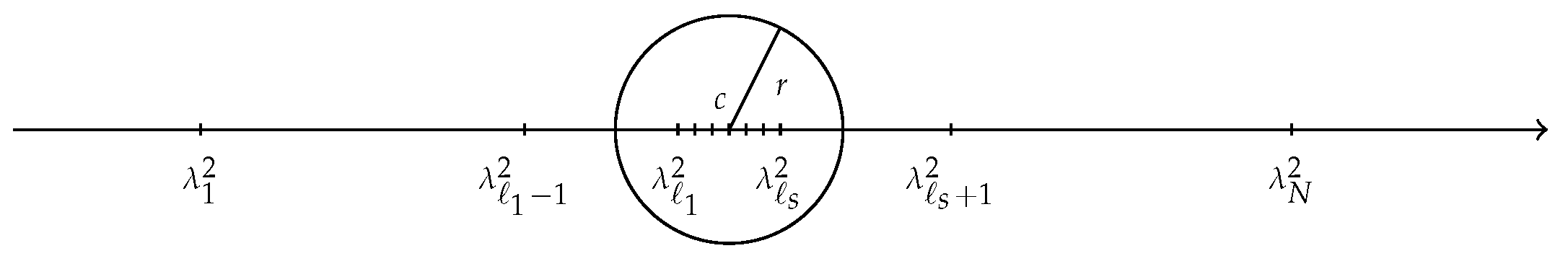
For LREP, suppose for are all the wanted eigenvalues whose square are inside the circle with center at c and radius r on the complex plane, as illustrated in the following Figure 1.
Given a random matrix , for any filter function that serves the purpose of filtering out the unwanted eigen-directions, we have, by Lemma 2,
As we known in [10], the ideal filter for computing for should map all s wanted eigenvalues to one and all unwanted ones to zero. For such a purpose, we also consider the filter function applied in [17], i.e.,
By Cauchy’s residue theorem [26] in complex analysis, we have:
As stated in [24] [Lemma 1], the matrix , with probability one, is nonsingular if the entries of Y are random numbers from a continuous distribution and they are independent and identically distributed. Therefore, naturally, the columns of span the invariant subspace of corresponding to for . However, it needs to calculate the contour integral. In practice, this is done by using numerical quadratures to compute this filter approximately. It is noted that for are all real. Let for . Then, we have:
where stands for the real part. A q-point interpolatory quadrature rule, such as the trapezoidal rule or Gauss–Legendre quadrature, leads to:
where and are the quadrature nodes and weights, respectively, and for . Let . Then, by (6), V is computed by solving shifted linear systems of the form:
Furthermore, for any interpolatory quadrature rule, we have by [18] that:
It follows by Lemma 3 that if the columns of V span the y-component of an approximate invariant subspace of H, then the columns of should span the x-component of the same approximate invariant subspace. Therefore, {, } is a pair of approximated deflating subspaces of H. By [3], the best approximations of for with the pair of approximate deflating subspaces {, } are eigenvalues of:
where and are two nonsingular factors of . In particular, we choose where is ’s Cholesky decomposition. This leads to:
Let the eigenvalues of G be in ascending order and the associated eigenvectors be , i.e., for . Then,
Approximating eigenpairs of H is then taken to be (, ) where:
We summarize the pseudo-code of the FEAST algorithm for LREP in Algorithm 1. A few remarks regarding Algorithm 1 are in order:
Remark 1.
(a) In practice, we do not need to save , and for every i in Algorithm 1. In fact, the subscript “” is just convenience for the convergence analysis in the next subsection.
(b) Since the trapezoidal rule yields much faster decay outside than the Gauss–Legendre quadrature [23], our numerical examples use the trapezoidal rule to evaluate , i.e., in (6),
(c) In Algorithm 1, it usually is required to know the eigenvalue counts s inside the contour in advance. In practice, s is unknown a priori, and an estimator has to be used instead. Some available methods have been proposed in [27,28] to estimate eigenvalue counts, based on stochastic evaluations of:
(d) In our numerical implementation of Algorithm 1, we monitor the convergence of a computed eigenpair by its normalized relative residual norm:
The approximate eigenpair is considered as converged when:
where , , and ε is a preset tolerance.
| Algorithm 1 The FEAST algorithm for LREP. |
| Input: Given an initial block . Output: Converged approximated eigenpairs . 1: for , until convergence do 2: Compute by (6), and . 3: Compute , , , and . 4: Compute the spectral decomposition and approximate eigenpairs where by (9) for . 5: If convergence is not reached then go to Step 2, with . 6: end for |
3.2. Convergence Analysis
Without loss of generality, we suppose in this subsection:
and use the following simplifying notation:
In Algorithm 1, for a given scalar k, naturally, we would use as approximations to and as approximations to . In this subsection, we will investigate how good such approximations may be. Notice that is invertible since for by (8).
Lemma 5.
Suppose is nonsingular. Then, is full column rank for all i in Algorithm 1.
Proof.
We prove this statement by induction. If is invertible for some j, then:
where is nonsingular. Thus, has full column rank. This leads to and both being invertible. By Step 5 of Algorithm 1, we have , which is also full column rank. Furthermore,
is nonsingular. We conclude by induction that is full column rank for □
Theorem 1.
Suppose the condition of Lemma 5 holds. For , there exist where and such that, for any k,
Proof.
As we know in [29], an important quantity for the convergence properties of projection methods is the distance of the exact eigenspace from the search subspace. Theorem 1 establishes bounds on M-canonical angles from to the search subspace and -canonical angles from to the search subspace , respectively, to illustrate the effectiveness of the FEAST algorithm for LREP. As stated in [18], if the spectrum of is distributed somewhat uniformly, then we would expect to be as small as . That means and at a rate of Based on Theorem 1, the following theorem is obtained to bound the M-canonical angles between and and the -canonical angles between and , respectively.
Theorem 2.
Suppose the condition of Lemma 5 holds. Using the notations of Theorem 1, we have:
where:
and is the M-orthogonal projector onto .
Proof.
Let , and such that is M-orthogonal matrix, i.e.,
Then, we can write , where and . Furthermore, we have:
Now, we turn to bound the term . Notice that It follows by Lemma 2 that:
Multiply (19) by from the left to get:
Furthermore, we have:
By Lemma 4, we conclude that:
The inequality (15) is now a consequence of (17), (18), (20), and Theorem 1. Similarly we can prove (16). □
4. Numerical Examples
In this section, we present some numerical examples to illustrate the effectiveness of Algorithm 1 and the upper bounds in Theorem 1.
Example 1.
We first examine the upper bounds of Theorem 1. For simplicity, we consider diagonal matrices for K and M. Take with where:
In such a case, there are two eigenvalue clusters: and , and .
We seek the approximations associated with the first cluster and vary the parameter to control the tightness among eigenvalues. To make the numerical example repeatable, the initial block is chosen to be:
In such a way, satisfies the condition that is nonsingular. We run Algorithm 1 and check the bound for given by (11) with and , respectively. In Algorithm 1, the trapezoidal rule is applied to calculate with the parameters and . We compute the following factors:
in Table 1. From Table 1, we can see that, as η goes to zero, the bounds for are sharp and insensitive to η.
Example 2.
To test the effectiveness of Algorithm 1, we chose three test problems, i.e.,test1 totest3 in Table 2, which come from the linear response analysis for Na, Na, and silane (SiH4) compounds, respectively [9]. The matrices K and M oftest1,test2, andtest3 are both symmetric positive definite with order , 2834, and 5660, respectively. We compute the eigenvalues whose square lies in the interval (,) for and the associated eigenvectors by using the MATLAB parallel pool. The interval (,) and their corresponding eigenvalue counts for are detailed in Table 2. All our experiments were performed on a Windows 10 (64 bit) PC-Intel(R) Core(TM) i7-6700 CPU 3.40 GHz, 16 GB of RAM using MATLAB Version 8.5 (R2015a) with machine epsilon in double precision floating point arithmetic. In demonstrating the quality of computed approximations, we calculated the normalized residual norms defined in (10) and relative eigenvalues errors:
for the approximation eigenvalue where were computed by MATLAB’s function eig on H, and considered to be the “exact” eigenvalues for testing purposes.
In this example, we first investigated how the maximal relative eigenvalue errors and normalized residual norms, i.e., and in Table 3, respectively, changed for an increase in the number of quadrature points q in (6). We used the direct methods, such as Gaussian elimination, to solve the shifted linear systems (7) in this example. The numerical results of Algorithm 1 by running four FEAST iterations with q varying from four to nine are presented in Table 3. It is shown by Table 3 that the trapezoidal rule with 6, 7, or 8 quadrature nodes already achieved satisfactory results.
Notice that the wanted eigenvalues are inside the intervals presented in Table 2. The shift and invert strategy is usually not available for LREP since the traditional algorithms to calculate the partial spectrum of LREP, such as the methods proposed in [6,8], combined with the shift and invert strategy will lose the structure of (2).
In addition, as stated in [17], the FEAST algorithm can be cast as a direct technique in comparison to iterative Krylov subspace-type methods, because it is based on an exact mathematical derivation (5). Therefore, by dividing the whole spectrum of LREP into a number of disjoint intervals, the FEAST algorithm is able to compute all eigenvalues simultaneously on the parallel architectures. From this aspect, as [24], we compared Algorithm 1 with the MATLAB built-in function eig, which was used to compute all eigenvalues of H, and then, the target eigenvalues were selected in this example. Let the number of quadrature nodes and the convergence tolerance . Table 4 reports the total required CPU time in seconds of Algorithm 1 and eig fortest 1,test 2, andtest3, respectively. It is clear from Table 4 that Algorithm 1 was much faster than the MATLAB built-in function eig in this example. A similar comparison between the FEAST-type algorithms and the MATLAB built-in function eig in terms of timing can be found in [30,31].
Example 3.
As stated in Section 3, the implementation of Algorithm 1 involves solving several shifted linear systems of the form:
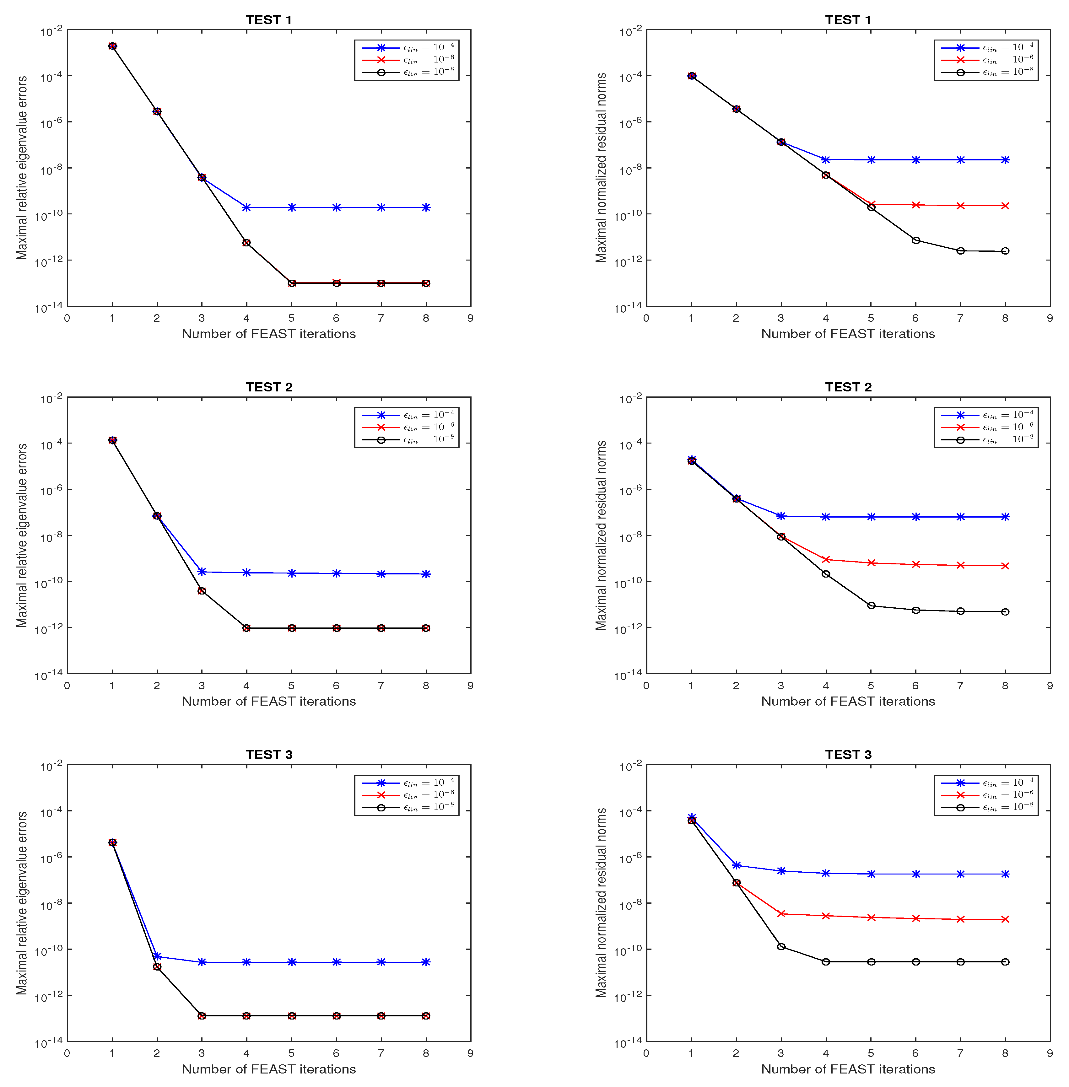
Direct solvers referring to operations are prohibitively expensive in solving large-scale sparse linear systems. Iterative methods, such as Krylov subspace-type methods [32], are usually preferred for large-scale sparse linear systems. However, Krylov subspace solvers may need a large number of iterations to converge. A way to speed up the FEAST method for LREP is to terminate the iterative solvers for linear systems before full convergence is reached. Therefore, in this example, we investigated the effect of the accuracy in the solution of linear systems on the relative eigenvalues errors and normalized residual norms. The linear systems were solved column-by-column by running GMRES [33] until:
Figure 2 plots the maximal relative eigenvalues errors and normalized residual norms of Algorithm 1 with in solvingtest 1,test 2, andtest 3with , , and . It is revealed by Figure 2 that the accuracy from the solution of the linear systems translated to the accuracy of the eigenpairs obtained by the FEAST algorithm for LREP; that is to say, higher accuracy in solving linear systems leads to better numerical performance in Algorithm 1. In particular, for a rather large , such as , it is hard to obtain satisfactory normalized residual norms in this example.
5. Conclusions
In this paper, we proposed a FEAST algorithm, i.e., Algorithm 1, for the linear response eigenvalue problem (LREP). The algorithm can effectively calculate the eigenvectors associated with eigenvalues that are located inside some preset intervals. Compared with other methods for LREP, the attractive computational advantage of Algorithm 1 is that it is easily parallelizable. We implemented numerical examples by using the MATLAB parallel pool to compute the eigenpairs in each interval independently of the eigenpairs in the other interval. The corresponding numerical results demonstrated that Algorithm 1 was fast and could achieve high accuracy. In addition, theoretical convergence results for eigenspace approximations of Algorithm 1 were established in Theorems 1 and 2. These theoretical bounds revealed the accuracy of the approximations of eigenspace. Numerical examples showed that the bounds provided by Theorem 1 were sharp.
Notice that the main computational tasks in Algorithm 1 consisted of solving q independent shifted linear systems with s right-hand sides. Meanwhile, as described above, the relative residual bounds in the solution of the inner shifted linear systems were translated almost one-to-one into the residuals of the approximate eigenpairs. Therefore, the subjects of further study include the acceleration of solving shifted linear systems on parallel architectures and theoretical analysis on how the accuracy of the inexact solvers in solving shifted linear systems interacts with the convergence behavior of the FEAST algorithm. In addition, while the algorithm in this paper is for real symmetric K and M, it is also available for the case of Hermitian K and M, simply by replacing all by (the set of complex numbers) and each matrix/vector transpose by the complex conjugate and transpose.
Author Contributions
Writing, original draft, Z.T.; writing, review and editing, Z.T. and L.L.
Funding
The work of the first author is supported in part by National Natural Science Foundation of China NSFC-11601081 and the research fund for distinguished young scholars of Fujian Agriculture and Forestry University No. xjq201727. The work of the second author is supported in part by the National Natural Science Foundation of China Grant NSFC-11671105.
Acknowledgments
The authors are grateful to the anonymous referees for their careful reading, useful comments, and suggestions for improving the presentation of this paper.
Conflicts of Interest
The authors declare no conflict of interest.
References
- Saad, Y.; Chelikowsky, J.R.; Shontz, S.M. Numerical methods for electronic structure calculations of materials. SIAM Rev. 2010, 52, 3–54. [Google Scholar] [CrossRef]
- Shao, M.; da Jornada, F.H.; Lin, L.; Yang, C.; Deslippe, J.; Louie, S.G. A structure preserving Lanczos algorithm for computing the optical absorption spectrum. SIAM J. Matrix Anal. Appl. 2018, 39, 683–711. [Google Scholar] [CrossRef]
- Bai, Z.; Li, R.C. Minimization principle for linear response eigenvalue problem, I: Theory. SIAM J. Matrix Anal. Appl. 2012, 33, 1075–1100. [Google Scholar] [CrossRef]
- Li, T.; Li, R.C.; Lin, W.W. A symmetric structure-preserving ΓQR algorithm for linear response eigenvalue problems. Linear Algebra Appl. 2017, 520, 191–214. [Google Scholar] [CrossRef]
- Wang, W.G.; Zhang, L.H.; Li, R.C. Error bounds for approximate deflating subspaces for linear response eigenvalue problems. Linear Algebra Appl. 2017, 528, 273–289. [Google Scholar] [CrossRef]
- Bai, Z.; Li, R.C. Minimization principle for linear response eigenvalue problem, II: Computation. SIAM J. Matrix Anal. Appl. 2013, 34, 392–416. [Google Scholar] [CrossRef]
- Papakonstantinou, P. Reduction of the RPA eigenvalue problem and a generalized Cholesky decomposition for real-symmetric matrices. Europhys. Lett. 2007, 78, 12001. [Google Scholar] [CrossRef]
- Teng, Z.; Li, R.C. Convergence analysis of Lanczos-type methods for the linear response eigenvalue problem. J. Comput. Appl. Math. 2013, 247, 17–33. [Google Scholar] [CrossRef]
- Teng, Z.; Zhang, L.H. A block Lanczos method for the linear response eigenvalue problem. Electron. Trans. Numer. Anal. 2017, 46, 505–523. [Google Scholar]
- Teng, Z.; Zhou, Y.; Li, R.C. A block Chebyshev-Davidson method for linear response eigenvalue problems. Adv. Comput. Math. 2016, 42, 1103–1128. [Google Scholar] [CrossRef]
- Rocca, D.; Lu, D.; Galli, G. Ab initio calculations of optical absorpation spectra: solution of the Bethe-Salpeter equation within density matrix perturbation theory. J. Chem. Phys. 2010, 133, 164109. [Google Scholar] [CrossRef] [PubMed]
- Shao, M.; Felipe, H.; Yang, C.; Deslippe, J.; Louie, S.G. Structure preserving parallel algorithms for solving the Bethe-Salpeter eigenvalue problem. Linear Algebra Appl. 2016, 488, 148–167. [Google Scholar] [CrossRef]
- Vecharynski, E.; Brabec, J.; Shao, M.; Govind, N.; Yang, C. Efficient block preconditioned eigensolvers for linear response time-dependent density functional theory. Comput. Phys. Commun. 2017, 221, 42–52. [Google Scholar] [CrossRef] [Green Version]
- Zhong, H.X.; Xu, H. Weighted Golub-Kahan-Lanczos bidiagonalization algorithms. Electron. Trans. Numer. Anal. 2017, 47, 153–178. [Google Scholar] [CrossRef]
- Zhong, H.X.; Teng, Z.; Chen, G. Weighted block Golub-Kahan-Lanczos algorithms for linear response eigenvalue problem. Mathematics 2019, 7. [Google Scholar] [CrossRef]
- Bai, Z.; Li, R.C.; Lin, W.W. Linear response eigenvalue problem solved by extended locally optimal preconditioned conjugate gradient methods. Sci. China Math. 2016, 59, 1–18. [Google Scholar] [CrossRef]
- Polizzi, E. Density-matrix-based algorithm for solving eigenvalue problems. Phys. Rev. B 2009, 79, 115112. [Google Scholar] [CrossRef] [Green Version]
- Tang, P.T.P.; Polizzi, E. FEAST as a subspace iteration eigensolver accelerated by approximate spectral projection. SIAM J. Matrix Anal. Appl. 2014, 35, 354–390. [Google Scholar] [CrossRef]
- Kestyn, J.; Polizzi, E.; Tang, P.T.P. FEAST eigensolver for non-Hermitian problems. SIAM J. Sci. Comput. 2016, 38, S772–S799. [Google Scholar] [CrossRef]
- Gavin, B.; Miedlar, A.; Polizzi, E. FEAST eigensolver for nonlinear eigenvalue problems. J. Comput. Sci. 2018, 27, 107–117. [Google Scholar] [CrossRef] [Green Version]
- Krämer, L.; Di Napoli, E.; Galgon, M.; Lang, B.; Bientinesi, P. Dissecting the FEAST algorithm for generalized eigenproblems. J. Comput. Appl. Math. 2013, 244, 1–9. [Google Scholar] [CrossRef]
- Guttel, S.; Polizzi, E.; Tang, P.T.P.; Viaud, G. Zolotarev quadrature rules and load balancing for the FEAST eigensolver. SIAM J. Matrix Anal. Appl. 2015, 37, A2100–A2122. [Google Scholar] [CrossRef]
- Ye, X.; Xia, J.; Chan, R.H.; Cauley, S.; Balakrishnan, V. A fast contour-integral eigensolver for non-Hermitian matrices. SIAM J. Matrix Anal. Appl. 2017, 38, 1268–1297. [Google Scholar] [CrossRef]
- Yin, G.; Chan, R.H.; Yeung, M.C. A FEAST algorithm with oblique projection for generalized eigenvalue problems. Numer. Linear Algebra Appl. 2017, 24, e2092. [Google Scholar] [CrossRef] [Green Version]
- Li, R.C.; Zhang, L.H. Convergence of the block Lanczos method for eigenvalue clusters. Numer. Math. 2015, 131, 83–113. [Google Scholar] [CrossRef]
- Stein, E.M.; Shakarchi, R. Complex Analysis; Princeton University Press: New Jersey, NJ, USA, 2010. [Google Scholar]
- Futamura, Y.; Tadano, H.; Sakurai, T. Parallel stochastic estimation method of eigenvalue distribution. J. SIAM Lett. 2010, 2, 127–130. [Google Scholar] [CrossRef] [Green Version]
- Napoli, E.D.; Polizzi, E.; Saad, Y. Efficient estimation of eigenvalue counts in an interval. Numer. Linear Algebra Appl. 2016, 23, 674–692. [Google Scholar] [CrossRef] [Green Version]
- Saad, Y. Numerical Methods for Large Eigenvalue Problems: Revised Version; SIAM: Philadelphia, PA, USA, 2011. [Google Scholar]
- Yin, G. A harmonic FEAST algorithm for non-Hermitian generalized eigenvalue problems. Linear Algebra Appl. 2019, 578, 75–94. [Google Scholar] [CrossRef]
- Yin, G. On the non-Hermitian FEAST algorithms with oblique projection for eigenvalue problems. J. Comput. Appl. Math. 2019, 355, 23–35. [Google Scholar] [CrossRef]
- Saad, Y. Iterative Methods for Sparse Linear Systems; SIAM: Philadelphia, PA, USA, 2003. [Google Scholar]
- Saad, Y.; Schultz, M.H. GMRES: A generalized minimal residual algorithm for solving nonsymmetric linear systems. SIAM J. Sci. Comput. 1986, 7, 856–869. [Google Scholar] [CrossRef]
Figure 1.
Schematic representation of the wanted eigenvalues.

Figure 2.
Convergence behavior of Algorithm 1 for test 1, test 2, and test 3 with , , and , respectively.
Figure 2.
Convergence behavior of Algorithm 1 for test 1, test 2, and test 3 with , , and , respectively.


Table 1.
together with their corresponding upper bounds of Example 1.
| (for ) | () | () | () | |
|---|---|---|---|---|
Table 2.
Test matrices.
| Problem | N | K | M | (, ) | (, ) | (, ) | |||
|---|---|---|---|---|---|---|---|---|---|
| test 1 | 1862 | Na | Na | (0.40,0.50) | 3 | (0.60,0.70) | 3 | (1.50,1.60) | 3 |
| test 2 | 2834 | Na | Na | (0.03,0.04) | 4 | (0.05,0.06) | 4 | (0.32,0.33) | 5 |
| test 3 | 5660 | SiH4 | SiH4 | (0.25,0.30) | 3 | (0.75,0.80) | 6 | (1.75,1.80) | 8 |
Table 3.
Changes of and with the number of quadrature nodes q varying from 4 to 9.
| q | TEST 1 | TEST 2 | TEST 3 | |||
|---|---|---|---|---|---|---|
| 4 | ||||||
| 5 | ||||||
| 6 | ||||||
| 7 | ||||||
| 8 | ||||||
| 9 | ||||||
Table 4.
Comparison of Algorithm 1 and eig for CPU time in seconds.
| Problem | eig | Algorithm 1 |
|---|---|---|
| test 1 | 45.82 | 15.88 |
| test 2 | 159.77 | 37.08 |
| test 3 | 1200.71 | 233.12 |
© 2019 by the authors. Licensee MDPI, Basel, Switzerland. This article is an open access article distributed under the terms and conditions of the Creative Commons Attribution (CC BY) license (http://creativecommons.org/licenses/by/4.0/).
Share and Cite
MDPI and ACS Style
Teng, Z.; Lu, L. A FEAST Algorithm for the Linear Response Eigenvalue Problem. Algorithms 2019, 12, 181. https://0-doi-org.brum.beds.ac.uk/10.3390/a12090181
AMA Style
Teng Z, Lu L. A FEAST Algorithm for the Linear Response Eigenvalue Problem. Algorithms. 2019; 12(9):181. https://0-doi-org.brum.beds.ac.uk/10.3390/a12090181
Chicago/Turabian StyleTeng, Zhongming, and Linzhang Lu. 2019. "A FEAST Algorithm for the Linear Response Eigenvalue Problem" Algorithms 12, no. 9: 181. https://0-doi-org.brum.beds.ac.uk/10.3390/a12090181
Note that from the first issue of 2016, this journal uses article numbers instead of page numbers. See further details here.