Multi-Fidelity Gradient-Based Strategy for Robust Optimization in Computational Fluid Dynamics

Abstract

Efficient Robust Design Optimization (RDO) strategies coupling a parsimonious uncertainty quantification (UQ) method with a surrogate-based multi-objective genetic algorithm (SMOGA) are investigated for a test problem in computational fluid dynamics (CFD), namely the inverse robust design of an expansion nozzle. The low-order statistics (mean and variance) of the stochastic cost function are computed through either a gradient-enhanced kriging (GEK) surrogate or through the less expensive, lower fidelity, first-order method of moments (MoM). Both the continuous (non-intrusive) and discrete (intrusive) adjoint methods are evaluated for computing the gradients required for GEK and MoM. In all cases, the results are assessed against a reference kriging UQ surrogate not using gradient information. Subsequently, the GEK and MoM UQ solvers are fused together to build a multi-fidelity surrogate with adaptive infill enrichment for the SMOGA optimizer. The resulting hybrid multi-fidelity SMOGA RDO strategy ensures a good tradeoff between cost and accuracy, thus representing an efficient approach for complex RDO problems.

1. Introduction

In recent years, robust design optimization (RDO) [1] has received increasing interest in engineering applications, due to its ability to provide efficient designs with a stable behavior under uncertainties of a diverse nature, such as randomly fluctuating operating conditions, geometric tolerances, and model uncertainties. Taguchi’s method [2], relying on the simultaneous optimization of the average and variance of the stochastic cost functions, is by far the most popular RDO method, although approaches allowing accounting for rare events, such as the low-quantile [3,4] or the “horsetail matching” [5] methods, have been paid significant interest recently.

The main ingredient for RDO is an uncertainty quantification (UQ) method, allowing characterizing the probability distribution functions (pdf) or, at least, the lower order statistics of the cost functionals for each proposed design, in order to select those that guarantee the best possible average performance while avoiding critical deviations when nominal design conditions are not matched. According to the RDO method in use, a single objective deterministic design problem is generally converted into a multi-objective (Pareto front) one, with the aim to optimize the average performance while avoiding critical performance loss at off-design conditions. For this reason, RDO often combines an UQ solver with evolutionary algorithms (typically, multi-objective genetic algorithms (MOGA) [6,7]), which are naturally suited for providing a full set of compromise solutions among the multiple objectives. On the other hand, evolutionary optimizers are generally very demanding in terms of cost function evaluations, which may require in the end a prohibitive computational effort for problems described by costly computer models, such as those encountered in computational fluid dynamics (CFD), despite the use of massive parallelization [8,9,10]. In order to reduce the number of costly function calls, it is crucial to select parsimonious UQ methods and optimizers, the overall cost of RDO being typically the product of the cost of the two approaches [11]. Past examples of RDO in CFD include various forms of UQ solvers based on non-intrusive polynomial chaos expansion [11,12] or surrogate models such as simplex stochastic collocation [13] or kriging [9]. All of them require a number of CFD solves quickly increasing with the number of uncertain parameters, and their direct coupling with MOGA optimizers is not computationally affordable for industrial applications, especially if massively parallel computers are not available.

An interesting option for reducing the cost of UQ solves is to use gradient information. A simple method for approximating statistical moments of the cost function by Taylor series expansions is the so-called first-order method of moments (MoM) [14]. Such a method can be remarkably fast if the derivatives of the cost function with respect to the uncertain variables are readily available by means of a discrete or continuous adjoint solver [15,16,17,18,19,20]. Nevertheless, its accuracy is limited to Gaussian or weakly non-Gaussian processes with small uncertainties, since higher-order terms become increasingly important for strongly non-Gaussian input distributions. Some improvement can be achieved by using higher-order expansions, but these require information about higher-order sensitivity derivatives, which may represent a delicate and highly intrusive task. A more complete discussion can be found in [21]. An alternative to MoM, better suited for high uncertainty ranges and generic pdf, consists of leveraging gradient information to construct a high-quality surrogate from a reduced number of samples. Such an approach is used for instance in gradient-enhanced kriging (GEK) surrogates [22,23,24]. Once the surrogate is available, inexpensive Monte Carlo sampling on the response surface can be used to estimate the required statistics.

Massive parallelization is of great help for speeding up the RDO process [10,11,25], but it is not promptly applicable for routine industrial use. A way of drastically reducing the required number of function calls consists of replacing the costly CFD or UQ solvers with surrogate models, such as radial basis functions [26], artificial neural networks [27], and kriging [9,10], approximating variations of the cost functions through the design space. Such an approach is called a surrogate-based multi-objective genetic algorithm (SMOGA).

Further reductions of computational time can be achieved by combining models with various levels of fidelity during the optimization. Such so-called multi-fidelity (MF) models [28,29] leverage the use of inexpensive, but low-fidelity (LF) models for efficiently exploring the design or stochastic spaces, while using parsimonious high-fidelity (HF) samples to improve model accuracy. Examples of LF models are given by coarse-grid approximations [30,31,32,33], data-fit interpolation and regression models [34], projection-based reduced models [35,36], machine-learning-based models [37], or simplified models relying on approximations of the underlying physics [38,39,40]. In addition to an LF and an HF model, a correlation model is also required for combining data with various fidelity levels. A simple approach consists of linking the HF and the LF models by means of an additive correlation [41]: given an LF model $f_{LF}\left(\xi \right)$ and an HF model $f_{HF}\left(\xi \right)$, it is assumed that $f_{HF}\left(\xi \right)=f_{LF}\left(\xi \right)+\delta \left(\xi \right)$ where $\delta \left(\xi \right)$ is an error function to be estimated. This approach is accurate enough when HF and LF models have similar scales and a good correlation, as is the case for coarse-grid approximations [42]. As an alternative, a multiplicative correlation can be used [43,44,45]: $f_{HF}\left(\xi \right)=\rho \left(\xi \right)f_{LF}\left(\xi \right)$, with $\rho \left(\xi \right)$ a constant scalar multiplier. A more comprehensive formulation combining the preceding ones was proposed in [32]: $f_{HF}\left(\xi \right)=\rho f_{LF}\left(\xi \right)+\delta \left(\xi \right)$. This approach is considerably more robust, and it has been extensively used in conjunction with Gaussian process approximation (including kriging) and Bayesian inference [46,47,48,49]). More sophisticated correlations exist [50,51,52], but they may be difficult to implement for complex problems.

In the present paper, we build on a SMOGA-based RDO technique introduced in [10], relying on the coupling of two nested Bayesian kriging (BK) surrogates: the first one is used to compute the required statistics of the objective functions in the uncertain parameter space, while the second one is used to model the response of these statistics to the design variables. Such an approach is called “combined kriging” [53]. An expected improvement criterion is used to update the second kriging surrogate during convergence towards the optimum. This technique has been successfully applied to the design of turbine blades for organic Rankine cycles [9] and to the RDO of the thermodynamic cycle [54]. Assuming that each kriging surrogate requires a number of samples approximately equal to 10 times the cardinality of the parameter space to build a reasonably accurate approximation [55], the nested BK RDO strategy needs $\mathcal{O}(100\times n_{unc}\times n_{des})$ function evaluations (with $n_{unc}$ the number of uncertain parameters and $n_{des}$ the number of design variables) in the first generation of the GA to generate the initial kriging surrogates for the statistical moments. Additional $\mathcal{O}(10\times n_{unc})$ evaluations are required for each update of the external kriging surrogate. Such a number of function calls is still too expensive for industrial CFD problems, even for uncertain or design spaces of low to moderate dimensionality (up to about eight uncertain or design parameters). GEK surrogates can be used to reduce the number of samples for the UQ step, but GEK-based MOGA is not straightforward in the context of RDO problems, since it requires also the gradient of the statistical moments of the QoI’s pdf with respect to the design variables. Obtaining such a piece of information by using efficient adjoint methods is not a trivial task; on the other hand, finite difference approximations are easily applicable, but at the price of a considerable computational expense for high-dimensional design spaces.

This is why we propose in this work a new multi-fidelity strategy for RDO that drastically reduces the required number of function calls by leveraging an inexpensive (but low-accuracy) first-order method of moments (MoM) and a Bayesian GEK [56]. Using gradient-based solvers allows reducing per se the number of function solves in the UQ step and to mitigate the curse of dimensionality. Here, the two models are fused together by using a methodology similar to [57] to generate a surrogate model for the MOGA optimization that combines the efficiency of MoM and the accuracy of GEK. The surrogate is enriched based on the expected improvement criterion during MOGA convergence, as in [9]. The required gradient information is obtained by using either continuous or discrete adjoint formulations. The new MF-RDO strategy is applied to an inexpensive test problem, i.e., the stochastic inverse design of a supersonic quasi-1D nozzle. The results show that a few GEK UQ solves are sufficient to correct the MoM solution, thus reducing the computational cost of the RDO by approximately one order of magnitude with respect to the nested BK strategy. Computational gains are expected to be even more substantial for costly industrial CFD problems.

The paper is organized as follows. In Section 2, we present the RDO problem and the test problem. The UQ methods considered in the study are described in Section 3. Section 4 presents the surrogate-based and multi-fidelity RDO strategies. In Section 5, we first apply various UQ methods to the test configuration and compare their accuracy and computational costs; afterwards, such methods are combined with a SMOGA or MF-SMOGA, and their efficiency in solving the RDO problem is assessed. Conclusions and final remarks are reported in Section 6.

2. Problem Definition

Following Taguchi’s RDO method, we look for a methodology allowing optimizing a set of QoIs, $\mathit{J}=\mathit{J}(\mathit{x},\xi )$, $\mathit{J}\in {\mathbb{R}}^m$ depending on a vector of deterministic design parameters $\mathit{x}\in {\mathbb{R}}^{n_{des}}$ and on a vector of uncertain parameters $\xi \in {\mathbb{R}}^{n_{unc}}$. Note that some of the design parameters may also be uncertain. We formulate the RDO problem by using the expectancy and the variance of J as measures of robustness, which leads to the solution of the two objective deterministic optimization problem in Equation (1).

$${\min }_{\mathit{x}}E\left[\mathit{J}\right],{\min }_{\mathit{x}}var\left[\mathit{J}\right]$$

(1)

The preceding optimization problem is solved by means of an MOGA. More precisely, following our previous studies [10,12], we adopt the non-dominated sorting genetic algorithm (NSGA-II) of Deb et al. [58], which provides an approximated Pareto front of optimal solutions corresponding to different trade-offs between average performance and robustness for the various QoIs at hand. For simplicity, in the following, we consider only the case of a single QoI, $m=1$, but the approach can be extended to multiple QoIs. The required statistics of the QoIs are calculated by means of a non-intrusive UQ method, which, for CFD models, is coupled with a suitable (costly) flow solver. Thus, the first ingredient of the RDO process is an efficient UQ approach, which provides accurate approximations of $E\left[\mathit{J}\right]$ and $var\left[\mathit{J}\right]$ based on a set of N deterministic samples of the solution. The UQ methods investigated in this work are described in Section 3.

Direct coupling of the MOGA with the UQ solver is overly costly for CFD, due to the high number of function evaluations. For instance, running the MOGA with a population of $n_{pop}$ individuals over $n_{gen}$ generations and using N samples for UQ lead to an overall number of CFD evaluations of the QoI of about $N\times n_{pop}\times n_{gen}$. The computational cost can be greatly alleviated by running $N\times n_{pop}$ deterministic runs in parallel at each NSGA generation [8,25], but: (i) the required number of computational cores may exceed the computational resources available, and (ii) even with a perfect parallel scaling at each generation, the turn-around time of the RDO equals at least the average cost of a CFD run multiplied by $n_{gen}$. To reduce the computational cost, a second (external) surrogate model is introduced to predict the response of the cost functions to the design parameters, as described in Section 4.

2.1. Test Problem: Quasi-1D Supersonic Nozzle

Various RDO strategies are assessed against an inexpensive test problem (also studied in [10,17]), namely the inverse design of a supersonic quasi-1D diverging nozzle. This allows validating UQ methods against MC sampling.

The nozzle geometry is assigned through the area distribution $S\left(x\right)$ along the longitudinal axis x. This is chosen to be of the form:

$$S\left(x\right)=a+btanh(cx-d)$$

(2)

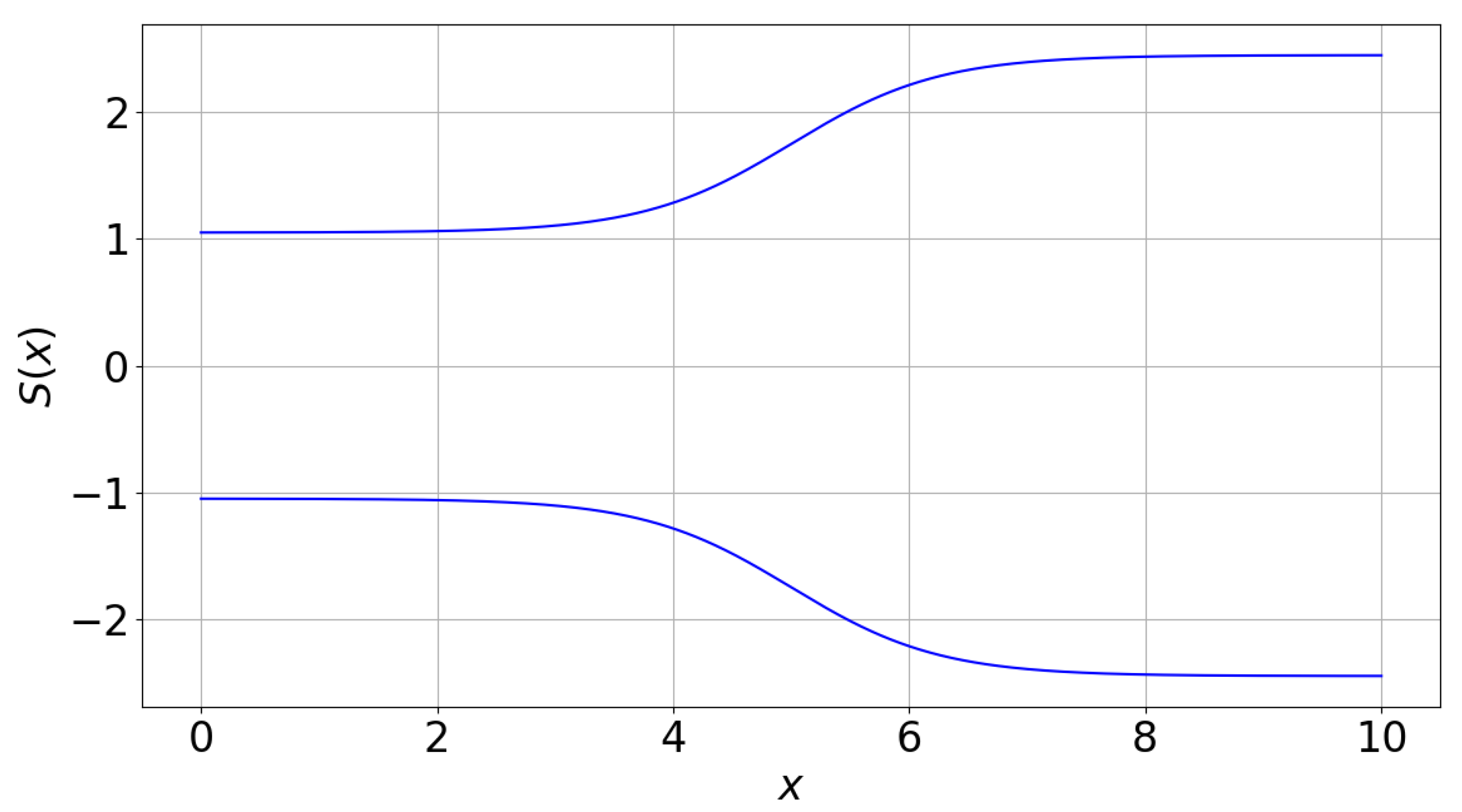
with a, b, c, and d coefficients defining the geometry. The nozzle length is set to $L=10$. A typical nozzle geometry is depicted in Figure 1.

For this test case, the QoI J (Equation (3)) is a scalar, namely the mean quadratic error of the actual pressure distribution in the nozzle $P\left(x\right)$ with respect to the target design pressure distribution $P_{des}\left(x\right)$. The latter corresponds to the pressure distribution for a nozzle geometry with $a=1.75$, $b=0.699$, $c=1.00$, and $d=3.80$, a reservoir pressure $P_{T,in}=1$ bar, an outlet static pressure $P_{out}=0.6$ bar, and a gas specific heat capacity ratio $\gamma =1.4$.

$$J=\frac{1}{2}{\int }_0^L{(P-P_{des})}^{2}dx$$

(3)

The optimization goal is to determine the design parameters $a,b,c,d$ in Equation (2) providing the best fit to the target pressure distribution under multiple uncertainties, in the sense of Equation (1).

The flow is assumed to be governed by the steady Euler equations for quasi-1D flows (Equation (4)):

$$R(w,x)=\frac{\partial \left(fS\right)}{\partial x}+K\frac{dS}{dx}=0$$

(4)

where $w={[\rho ,\rho v,\rho e_t]}^T$ and $f\left(w\right)={[\rho v,\rho v^2+P,\rho v{h}_t]}^T$ are, respectively, the conservative variable and the physical flux vectors [59]. In the preceding equations, $\rho$ is the fluid density, v is the velocity along the nozzle axis, $e_t$ and $h_t$ are the total specific energy and enthalpy, and $K={[0,-P,0]}^T$. The system of equations is supplemented by the equation of state for thermally and calorically perfect gases, $P=(\gamma -1)\rho (e_T-v^2/2)$. The governing equations are discretized by a cell-centered finite volume formulation, using Rusanov’s first-order upwind scheme for space integration. The steady state solution is computed iteratively by solving a false transient with four-stage explicit Runge–Kutta time-stepping [59]. Characteristic boundary conditions based on Riemann invariants are imposed at the nozzle inlet and outlet. Sonic flow conditions are prescribed at the inlet, so that all Riemann invariants enter the domain. The range of variation of the total pressure is such that a shock is always created in the divergent nozzle. As a consequence, outlet flow conditions are always subsonic. In this case, we impose the outlet static pressure, which is treated as deterministic, and fixed to $P_{out}=0.6$ bar. Based on a preliminary mesh study, a computational grid of 300 uniformly spaced cells is used in all of the following calculations.

The system is assumed to be subject to uncertainties of various nature, specifically:

• geometric tolerances on the nozzle shape, modeled by treating the shape parameters $a,b,c,d$ as normally distributed random variables, with mean $\mu$ and coefficient of variation $CoV=\sigma /\mu$, with $\sigma$ the standard deviation;
• uncertainties in inlet total pressure $P_{T,in}$ described as a uniformly-distributed random variable with imposed lower and upper bounds;
• uncertainties in the gas properties, here represented by the specific heat ratio $\gamma$, which is also assumed as uniformly distributed.

The characteristics of the random parameters are listed in

Table 1. Characteristics of the pdfs used to model the uncertain parameters.

Quantity	pdf Distribution	Distribution Parameters
a	Gaussian	$\mu \in$ [1.5–2.0],   $CoV=0.01$
b	Gaussian	$\mu \in$ [0.6–0.8],   $CoV=0.01$
c	Gaussian	$\mu \in$[0.7–0.9],   $CoV=0.01$
d	Gaussian	$\mu \in$ [3.9–4.1],   $CoV=0.01$
$P_{T,in}$	Uniform	[0.90–1.10]
$\gamma$	Uniform	[1.39–1.41]

. In the inverse design process, the uncertain geometric parameters are also (uncertain) design variables: for this reason, their mean is not fixed, but varies within the ranges corresponding to the bounds of the design space. This means that, even for designs corresponding to the upper/lower bounds, a realization of the nozzle geometry may lie outside the prescribed limits, due to geometric tolerances.

3. Uncertainty Quantification Methods

The goal of UQ methods is to estimate variability in the output of a model, corresponding to a set of QoIs, given variations in the model inputs. We present in the following two gradient-based UQ methods. The first one is a so-called probabilistic and non-intrusive approach, which predicts the approximate pdfs of the output QoIs, given the probability distributions assigned to the inputs and a set of samples of the QoI obtained by running the model as a black-box function. It relies on MC sampling on a gradient-enhanced kriging surrogate. The second one is a deterministic, more intrusive, approach based on Taylor-series expansion of the QoI with respect to the uncertain parameters, and it corresponds to a first-order adjoint method of moments (MoM). In addition to those UQ methods, we also consider a UQ solver based on the BK surrogate of [9], which does not use gradient information. BK is also used as the external surrogate model for SMOGA in the next section.

3.1. Bayesian Kriging and Gradient-Enhanced Kriging

Surface-response methods based on Bayesian kriging (BK) are implemented to achieve a non-intrusive estimate of the cost function statistics. In the following, we first introduce a BK formulation using only the observed values of the QoI $\mathit{J}$. Afterwards, we extend the formulation to account for gradient information, leading to Bayesian GEK.

3.1.1. Bayesian Kriging

A surface-response method based on BK was implemented to achieve a non-intrusive estimate of the cost function statistics. The QoI $\mathit{J}$ is modeled as a regression function of the form:

$$\mathit{J}\left(\xi \right)=\sum _i{f}_i\left(\xi \right){\beta }_i+Z\left(\xi \right)=m\left(\xi \right)+Z\left(\xi \right)$$

(5)

where we dropped the dependency on the deterministic quantities for simplicity, so that $\xi$ defines a generic point in the $n_{unc}$-dimensional uncertain space, $f_i$ are basis functions of the regression model, ${\beta }_i$ are regression coefficients to be determined, and $Z\left(\xi \right)$ is a zero mean Gaussian process (GP) [60], modeling the deviation between the regression function and the data. Choosing a zeroth-order polynomial as the regression model leads to the so-called ordinary kriging. The deviation Z is represented as a multi-variate normal distribution $Z\sim N(0,\mathit{R})$, with zero mean and covariance matrix $\mathit{R}$.

The kriging approximation can be formulated in a Bayesian statistical framework. In this case, the BK surrogate predicts a set of M values of the QoI $\mathit{J}\left(\xi \right)$, conditional on N observed data ${\mathit{J}}^{*}$, where ${\mathit{J}}^{*}$ is selected from the full set of J through the observation matrix $\mathit{H}$ of size $N\times M$: ${\mathit{J}}^{*}=\mathit{H}\mathit{J}$ with:

$$H_{ij}=\left\{\begin{array}{c}1,\mathrm{if}i=j\\ 0,\mathrm{otherwise}\end{array}\right.$$

(6)

for $i=1,...,M$ and $j=1,...,N$. The vector of the unknown QoI $\mathit{J}\left(\xi \right)$ is supposed to follow a normal prior distribution $p\left(\mathit{J}\right)$, $\mathit{J}$∼$N(0,\mathit{P})$, where the covariance matrix P has to be estimated. Besides, the conditional probability to observe the N data ${\mathit{J}}^{*}$ given the unknowns $\mathit{J}$ (known as the likelihood function) is also supposed to be a normal distribution of the form:

$${\mathit{J}}^{*}|\mathit{J}\sim N(\mathit{H}\mathit{J},\mathit{R})$$

(7)

The observation error is modeled as uniform and uncorrelated, resulting in a covariance matrix of the form $\mathit{R}={ϵ}^2\mathit{I}$, where I is the unit matrix and $ϵ$ a pre-specified error of the observed variable values. The posterior distribution of the unknowns, conditional to the observed data, can be inferred by means of the Bayes theorem, such that:

$$p\left(\mathit{J}\right|{\mathit{J}}^{*})\sim p\left({\mathit{J}}^{*}\right|\mathit{J})p\left(\mathit{J}\right)$$

(8)

The posterior being the product of two normal distributions results in being a normal distribution as well, whose parameters depend on the expression of the prior covariance $\mathit{P}$:

$$p\left(\mathit{J}\right|{\mathit{J}}^{*})\sim N(E\left[\mathit{J}|{\mathit{J}}^{*}\right],var\left[\mathit{J}|{\mathit{J}}^{*}\right])$$

(9)

Assuming that $\mathit{J}$ and ${\mathit{J}}^{*}$ are normalized such that ${\mathit{J}}^{*}$ has zero mean and unit variance, the covariance matrix $\mathit{P}$ of the prior distribution $p\left(\mathit{J}\right)$ is defined such that its elements are generated by the squared exponential kernel (reported below in the 1D case, for simplicity):

$$\mathbf{P}=cov(h_{ij},\theta )=\left[exp\left(-\frac{h_{ij}^2}{2{\theta }^2}\right)\right]$$

(10)

where $h_{ij}={\xi }_i-{\xi }_j$ is the correlation range, ${\xi }_i$ the generic coordinate of the observation point ${\mathit{J}}^{*}$, and $\theta$ a hyperparameter that has to be estimated (for multi-dimensional problems, it is a vector whose dimension is the cardinality of the parameter space). Following [61], the kriging predictor mean and variance are:

$$E\left(\mathit{J}\right|{\mathit{J}}^{*})=\mathit{P}{\mathit{H}}^T{(\mathit{R}+\mathit{H}\mathit{P}{\mathit{H}}^T)}^{-1}{\mathit{J}}^{*}$$

(11)

$$var\left(\mathit{J}\right|{\mathit{J}}^{*})=[\mathit{I}-\mathit{P}{\mathit{H}}^T{(\mathit{R}+\mathit{H}\mathit{P}{\mathit{H}}^T)}^{-1}]\mathit{P}$$

(12)

The advantage of this methodology is that the kriging variance provides a natural measure of the accuracy of the surrogate model. Because we deal with an ordinary kriging model where the hyperparameters need to be estimated, the maximum likelihood estimation (MLE) approach is implemented in order to evaluate the hyperparameter vector $\theta$ as the solution of the optimization problem:

$$ma{x}_{\theta }\left\{-\left(ln\left|\mathit{A}\right|+{\mathit{J}}^{*}T{\mathit{A}}^{-1}{\mathit{J}}^{*}\right)\right\}$$

(13)

where $\mathit{A}=(\mathit{R}+\mathit{H}\mathit{P}{\mathit{H}}^T)$. Since the optimization problem in (13) is defined over a multidimensional space of cardinality $n_{unc}$, whose cost grows as $\mathit{O}\left({\mathit{n}}_{\mathit{s}}{\mathit{N}}^{\mathit{3}}\right)$, where ${\mathit{n}}_{\mathit{s}}$ is the number of optimization steps and $\mathit{N}$ is the number of observed samples, it represents a bottleneck for the above methodology. The MLE problem is classically solved by means of the Nelder–Mead downhill simplex method [62]. Here, a global search algorithm based on a differential genetic evolution approach was implemented, providing an improvement in terms of computation time. Besides, efficient inversion of matrix $\mathit{A}$ is achieved through Cholesky decomposition.

Once the kriging surrogate has been trained from the data and the hyperparameters are estimated, the statistics of the QoI are calculated through Monte Carlo sampling of the kriging surface, according to some prescribed joint probability function distribution of the parameters $\xi$.

3.1.2. Gradient Enhanced Kriging

Bayesian kriging can be accelerated by adding gradient information. The formulation described hereafter is the form of so-called gradient-enhanced co-kriging, denoted GEK for simplicity, where the gradient data are added as covariables. This approach has been shown to be simpler and more robust for indirect gradient-enhanced kriging, where the gradient information is included in the surrogate by adding finite difference-based values at small distances from the sample locations, and then, a standard kriging is performed on the resulting augmented sample [22,23,24].

For the sake of clarity, we first describe GEK in the one-dimensional case: $J=J\left(\xi \right)$. Assuming that the derivatives of $dJ/d\xi$ are known at the M sampling points, the observation vector is redefined by concatenating the gradient information to the function values:

$${\mathit{J}}^{*}={\left({J_1}^{*},{J_2}^{*},\cdots ,{J_M}^{*},{{\displaystyle \frac{dJ}{d{\xi }^{*}}}{|}_1}^{*},{{\displaystyle \frac{dJ}{d{\xi }^{*}}}{|}_2}^{*},\cdots ,{{\displaystyle \frac{dJ}{d{\xi }^{*}}}{|}_M}^{*}\right)}^T$$

(14)

The covariance matrix is subsequently modified to account for the observational errors on the derivatives, also assumed to be uniform and uncorrelated. This results in a diagonal matrix of dimension $2M\times 2M$:

$$\mathbf{R}=diag(\underset{M\mathrm{times}}{\underbrace{{ϵ}^2,\cdots ,{ϵ}^2}},\underset{M\mathrm{times}}{\underbrace{{\varsigma }^2,\cdots ,{\varsigma }^2}})$$

(15)

where ${\varsigma }^2$ is the variance of the (identically distributed) observation errors on the gradients. Finally, the prior covariance is reformulated as in [63]:

$$\mathbf{P}=\left[\begin{array}{cc}{P}_{00}& P_{01}\\ P_{10}& P_{11}\end{array}\right]$$

(16)

with $P_{00}=cov(h_{ij},\theta )$,${\displaystyle P_{01}=\frac{\partial cov(h_{ij},\theta )}{\partial h_{ij}}}$,${\displaystyle P_{10}=-\frac{\partial cov(h_{ij},\theta )}{\partial h_{ij}}}$, and ${\displaystyle P_{11}=\frac{{\partial }^{2}cov(h_{ij},\theta )}{\partial h_{ij}^2}}$.

In the above, $P_{00}$ is the covariance of the function values, $P_{11}$ is the covariance of the derivatives, and $P_{01}$ and $P_{10}$ are the cross-covariances.

The GEK formulation is extended to M-dimensional problems in a straightforward manner: the observation vector is expanded by adding N M-dimensional gradients, which results in the $N\times (M+1)$ compiled observations [64]. The prior covariance $\mathbf{P}$ becomes:

$$\mathbf{P}=\left[\begin{array}{cccc}{P}_{00}& P_{01}& \cdots & P_{0M}\\ P_{10}& P_{11}& \cdots & P_{1M}\\ ⋮& ⋮& \ddots & ⋮\\ P_{M0}& P_{M1}& \cdots & P_{MM}\end{array}\right]$$

(17)

where:

$${\displaystyle P_{ij}^{kl}=\frac{{\partial }^{2}cov({\xi }_{k,j},{\xi }_{l,i})}{\partial {\xi }_k\partial {\xi }_l}}$$

(18)

Due to the use of additional gradient information, GEK achieves a given level of accuracy with a number of samples that is consistently lower than BK. However, the solution quality may be highly dependent on the accuracy of the computed gradients [24], which must be properly accounted for when building the surrogate.

3.2. Method of Moments

Among deterministic UQ methodologies, an interesting approach is the MoM, which approximates the statistical moments of the fitness function by Taylor series expansions. This method may provide fast and sufficiently accurate estimates of the QoI statistics, as long as the fitness sensitivity derivatives with respect to uncertain parameters are provided by an efficient method and complete output statistics are not required [17]. Both first- and second-order MoM formulations have been considered in the literature (see for instance [17]). Here, we restrict our attention to the first-order MoM, as a candidate low-fidelity UQ method to be combined with a higher-fidelity approach, as discussed later. Following [65], the first-order approximation for the expected value (mean) of J is simply given by:

$$E_{FO}\left[J\left(\xi \right)\right]=J\left(\overline{\xi }\right)$$

(19)

which is nothing but the deterministic evaluation of function J at the mean value of the input $\overline{\xi }$. The first-order variance is:

$$Va{r}_{FO}\left[J\left(\xi \right)\right]=\sum _{i=1}^N\sum _{j=1}^N\frac{\partial J}{\partial {\xi }_i}{|}_{\overline{\xi }}\frac{\partial J}{\partial {\xi }_j}{|}_{\overline{\xi }}cov({\xi }_i,{\xi }_j)$$

(20)

with $cov({\xi }_i,{\xi }_j)$ the covariance matrix. If the variables $\xi =\left\{{\xi }_1,{\xi }_2,....{\xi }_N\right\}$ are uncorrelated, the covariance is a diagonal matrix and Equation (20) takes the simplified form:

$$\begin{array}{cc}\hfill Va{r}_{FO}\left[J\left(\xi \right)\right]& =\sum _{i=1}^N\sum _{j=1}^N\frac{\partial J}{\partial {\xi }_i}{|}_{\overline{\xi }}\frac{\partial J}{\partial {\xi }_j}{|}_{\overline{\xi }}{\sigma }_i^2\hfill \end{array}$$

(21)

where ${\sigma }_i^2$ stands for the variance of the i-th uncertain parameter.

3.3. Gradient Calculation

The gradient information required for the GEK and MoM approaches is calculated by means of the adjoint method. Both the continuous and the discrete adjoint formulations are used in the following. Their derivation for the present quasi-1D nozzle problem is described in Appendix A.

4. Robust Design Optimization Strategy

As the RDO problem defined in Equation (1) is an intrinsically multi-objective problem, the well-known non-dominated sorting genetic algorithm NSGA-II [58] has been used as the optimizer. The MOGA requires evaluations of the RDO cost functions through the UQ method for each individual and for each generation. To reduce the computational cost of the RDO, one possibility is to construct a BK or GEK surrogate over a parameter space extended to the design variables, i.e., of dimensionality $n_{unc}+n_{des}$. Due to the curse of dimensionality, constructing a reliable surrogate over such a large parameter space may result in an unacceptable cost of the kriging approximation. To avoid this issue and to facilitate the use of gradient-based UQ, including MoM, we chose to construct instead a separate surrogate model mapping a variable in the design space to the cost function space.

4.1. BK-Based Robust Design Optimization

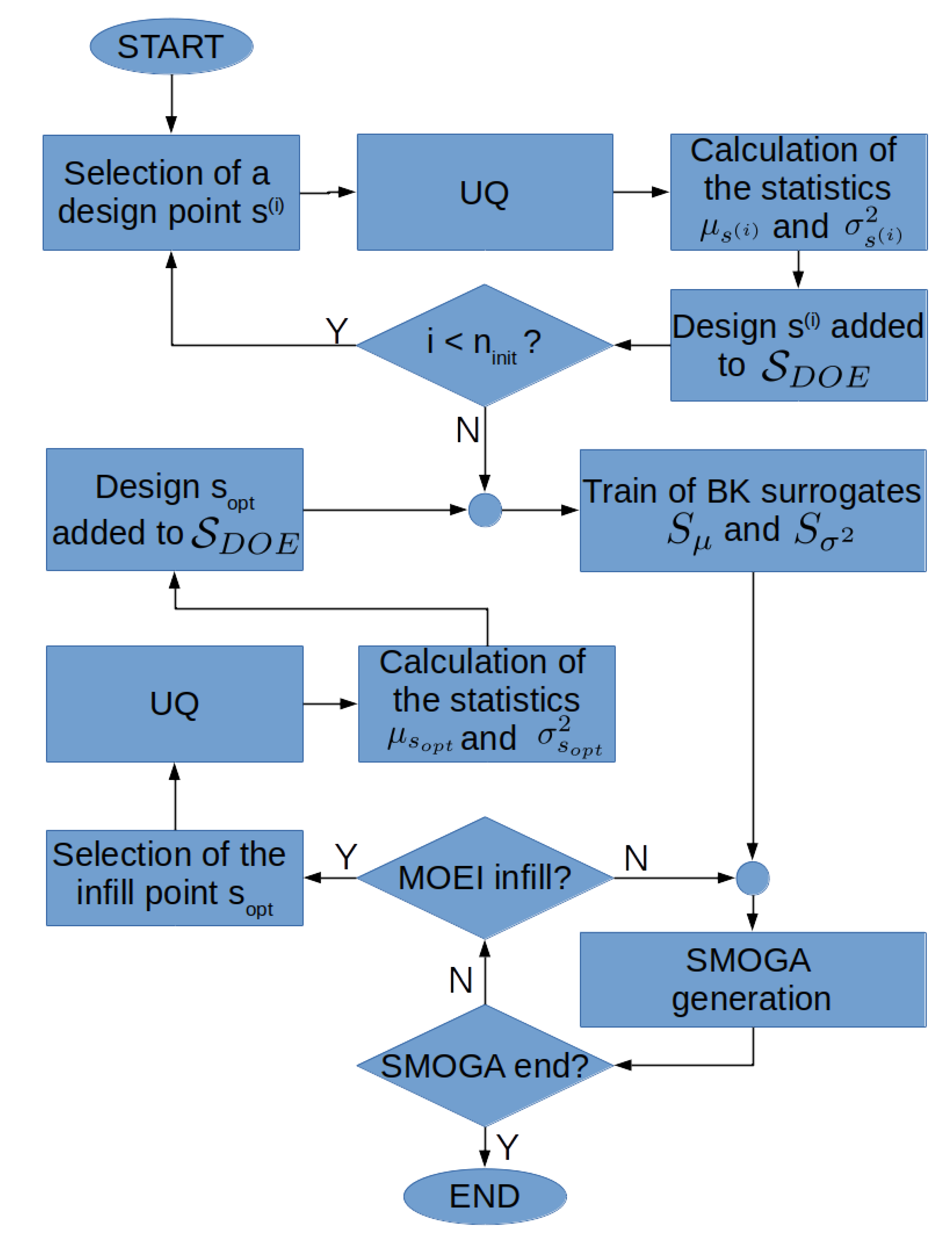
In [9,10,54], an external BK surrogate was constructed to describe variations of the mean and variance of the QoIs in the design space, by using $n_{init}$ samples chosen according to a preliminary design of experiments (DOE). In those references, a first-level UQ BK using N samples was used to evaluate the cost functions. In the present work, a similar approach is used, whereby a GEK surrogate or the MoM may replace first-level BK for the UQ step; a flowchart of the RDO process is provided in Figure 2.

The construction of the second-level surrogate requires $N\times n_{init}$ deterministic runs of the direct CFD solver in the case of BK and of the direct and adjoint solvers for GEK, which can be parallelized in a straightforward manner. The moderate extra-cost of adjoint solves for GEK is in general counter-balanced by a smaller N required for achieving a given accuracy. If the MoM is used as the UQ solver, the cost of the initial surrogate is reduced to $n_{init}$ deterministic runs of the direct (nonlinear) and adjoint CFD solvers. Numerical tests show that a sufficiently accurate BK surrogate can be obtained by setting $n_{init}=10n_{des}$. Once $n_{init}$ estimates of the QoI mean and variance have been obtained, a second-level BK is constructed and coupled with the MOGA. In order to control the accuracy of the approximated cost functions, an adaptive infill strategy is adopted to enrich the external BK surrogate during the evolution. For this purpose, we add to the initial new DOE samples selected during the MOGA iteration and retrain the BK model. Several infill criteria are available. For an overview about all these techniques the reader is addressed to [66,67]. Among them, the expected improvement (EI) criterion [68] has been shown to provide a good trade-off between exploitation and exploration, and it was therefore selected for the RDO carried out in the present work.

The new samples are drawn in such a way that the EI of the global minimum is maximized [69,70]. The EI quantifies the probability to improve the surrogate on the design space parameters. A global optimization of the EI function is then carried out to find the most suitable location for the new sample (see [70] for details).

Since RDO is intrinsically a multi-objective optimization process, the EI function is a surface of a hyper-dimensional parameter space, and a more complex formulation is developed, referred-to as the multi objective expected improvement (MOEI) approach (see [70]). The accuracy of the surrogate is rapidly improved with a few MOEI infills, so that ${\mathit{n}}_{\mathit{MOEI}}<<{\mathit{n}}_{\mathit{gen}}$. An MOEI update implies running the UQ algorithm for the additional sample to be integrated to the second-level BK. The N deterministic CFD and adjoint runs required for the BK and GEK UQ solvers can be carried out in parallel. Finally, the cost of the RDO based on the adaptive infill strategy in terms of cost-function evaluation is given by $N\times (n_{init}+n_{MOEI})$ direct CFD calculations for BK, $N\times (n_{init}+n_{MOEI})$ direct and adjoint CFD calculations for GEK, and $(n_{init}+n_{MOEI})$ direct and adjoint calculations for MoM. The turn-around time, in the case of a perfectly-scaling parallel implementation, is approximately equal to $n_{MOEI}+1$ runs. Based on numerical experiments, an MOEI adaptation every three to five MOGA generations is generally sufficient to achieve an accurate approximation of the optimum, as shown in the Results Section.

The full BK-based RDO loop is described in the pseudo-code provided hereafter in Algorithm 1.

Algorithm 1: BK RDO loop with the MOEI adaptation.

1. Initialization: LHS DOE with $n_{init}$ samples ${\mathcal{S}}_{DOE}=\left\{{\mathit{s}}^{\left(1\right)},{\mathit{s}}^{\left(2\right)},...,{\mathit{s}}^{\left(n_{init}\right)}\right\}$    While $i<n_{init}$    Select design ${\mathit{s}}^{\left(i\right)}$ in ${\mathcal{S}}_{DOE}$    Run UQ solver to compute the statistics ${\mu }_{s^{\left(i\right)}}$,${\sigma }_{s^{\left(i\right)}}^2$   Train surrogates ${\mathit{S}}_{\mu }\left({\mathcal{S}}_{DOE}\right)$, ${\mathit{S}}_{{\sigma }^2}\left({\mathcal{S}}_{DOE}\right)$   2. BK-SMOGA loop    While $n<n_{gen}$    If MOEI infill prescribed:      Solve MOEI pbto choose a new sample $s_{opt}$      Run UQ solver to compute ${\mu }_{s_{opt}}$, ${\sigma }_{s_{opt}}^2$      Re-train $S_{\mu }$, $S_{{\sigma }^2}$ by adding $s_{opt}$

4.2. Multi-Fidelity Methods for RDO

Although the BK-based SMOGA allows a considerable reduction of function calls during the RDO loop, the overall computational cost remains significant for high-dimensional design and uncertain spaces. While the computational cost is higher for BK or GEK solvers than for MoM, the former may provide an accurate estimate of the QoI statistics, which is not the case for the first-order MoM. With the aim of achieving a compromise between the accuracy of kriging-surrogate UQ solvers and the computational efficiency of the MoM, in this section, we introduce an advanced SMOGA, based on a multi-fidelity surrogate model of the design space replacing the preceding external BK surrogate (MF-SMOGA).

In the MF surrogate, the MoM UQ solver is used as the low-fidelity (LF) model, and the GEK UQ solver is the high-fidelity (HF) one. In the present implementation, an initial DoE is run at the first iteration of the SMOGA, where the HF and LF sampling points are generated independently. The auto-regressive correlation:

$$f_{HF}\left(\xi \right)=\rho f_{LF}\left(\xi \right)+\delta \left(\xi \right)$$

(22)

is used for correcting the discrepancy between the LF and HF models. More specifically, we follow the implementation proposed in [57], and we use the LF model as a basis function for the regression term expression of a universal kriging model; therefore, the term $m\left(\xi \right)$ in Equation (5) becomes:

$$m\left(\xi \right)=\sum _i{f}_i\left(\xi \right){\beta }_i+f_{LF}{\beta }_{\rho }$$

(23)

where ${\beta }_{\rho }$ is an estimate of the coefficient $\rho$ of Equation (22) by means of a GP regression. Assuming that the LF and HF models are independent, the mean ${\mu }_{HF}$ and variance ${\sigma }_{HF}^2$ of the high-fidelity model are given by:

$$\left\{\begin{array}{c}{\mu }_{HF}=\rho {\mu }_{LF}+{\mu }_{\delta }\hfill \\ {\sigma }_{HF}^2={\rho }^2{\sigma }_{LF}^2+{\sigma }_{\delta }^2\hfill \end{array}\right.$$

(24)

with ${\mu }_{LF}$, ${\sigma }_{LF}^2$, ${\mu }_{\delta }$, and ${\sigma }_{\delta }^2$ the means and variances of the LF model and of the discrepancy function $\delta$, respectively. In order to improve the MF surrogate accuracy during SMOGA convergence, adaptive infill based on the MOEI criterion is used. In this case, however, either the LF or the HF model can be used for the infill. In the following calculations, we adopt the strategy of [42]: for the infill, priority is given to the less expensive LF model, and the HF one is used only when improvement achieved with the lower level of fidelity is below a given tolerance, $tol={10}^{-4}$ in the present calculations. Either way, re-sampling at the same location is avoided.

Pseudo-code for the MF model is provided below in Algorithm 2; for more information about it, the reader is addressed to [57].

Algorithm 2: MF RDO loop with the MOEI adaptation.

1. Initialization:    LHS LF DOE with $n_{LF,init}$ samples ${\mathcal{S}}_{DOE,LF}=\left\{{\mathit{s}}_{LF}^{\left(1\right)},{\mathit{s}}_{LF}^{\left(2\right)},...,{\mathit{s}}_{LF}^{\left(n_{LF,init}\right)}\right\}$   LHS HF DOE with $n_{HF,init}<<n_{LF,init}$ samples ${\mathcal{S}}_{DOE,HF}=\left\{{\mathit{s}}_{HF}^{\left(1\right)},{\mathit{s}}_{HF}^{\left(2\right)},...,{\mathit{s}}_{HF}^{\left(n_{HF,init}\right)}\right\}$   While $i<n_{LF,init}$    Select design ${\mathit{s}}_{LF}^{\left(i\right)}$ in ${\mathcal{S}}_{DOE,LF}$    Run MoM solver to compute the statistics $\mu \left(s_{LF}^{\left(i\right)}\right)$, ${\sigma }^2\left(s_{LF}^{\left(i\right)}\right)$   Train LF surrogates ${\mathit{S}}_{LF,\mu }\left({\mathcal{S}}_{DOE,LF}\right)$, ${\mathit{S}}_{LF,{\sigma }^2}\left({\mathcal{S}}_{DOE,LF}\right)$    While $i<n_{HF,init}$    Select design ${\mathit{s}}_{HF}^{\left(i\right)}$ in ${\mathcal{S}}_{DOE,HF}$    Run GEK solver to compute the statistics $\mu \left(s_{HF}^{\left(i\right)}\right)$, ${\sigma }^2\left(s_{HF}^{\left(i\right)}\right)$   Use Equation (22) to construct MF surrogates: ${\mathit{S}}_{MF,\mu }\left({\mathcal{S}}_{DOE,HF}\right)$, ${\mathit{S}}_{MF,{\sigma }^2}\left({\mathcal{S}}_{DOE,HF}\right)$  2. MF-SMOGA loop    While $n<n_{gen}$    If MOEI infill prescribed:     Solve MOEI pb on MF surrogate to choose a new sample $s_{opt}$      If EI>tol:       Run MoM solver to compute ${\mu }_{s_{opt}}$,${\sigma }_{s_{opt}}^2$       Re-train $S_{MF,\mu }$,$S_{MF,{\sigma }^2}$ by adding $s_{opt}$      Else:       Run GEK solver to compute ${\mu }_{s_{opt}}$,${\sigma }_{s_{opt}}^2$       Re-train $S_{MF,\mu }$,$S_{MF,{\sigma }^2}$ by adding $s_{opt}$

5. Results

The quasi-1D supersonic nozzle test problem presented in Section 2.1 is first used to assess the BK, GEK, and MoM UQ methods against reference MC sampling. Afterwards, the methods are applied to a sample of nozzle geometries and used to build single or multi-fidelity surrogates used in the SMOGA RDO loop.

5.1. Preliminary Assessment of the UQ Methods

We select one of the nozzle geometries in the design space by assigning the geometric coefficients’ fixed normal pdfs with the standard deviation equal to 1% of the mean. The pdf parameters for the geometric variables are provided in

Table 2. Design parameters for the quasi-1D nozzle used for the assessment of the UQ techniques.

Design Parameter	pdf
a	∼$N(1.75,0.0175)$
b	∼$N(0.699,0.00699)$
c	∼$N(0.8,0.008)$
d	∼$N(4.00,0.004)$

. The operation and thermodynamic parameters are assigned the same pdf as in Table 1. The pdfs are sampled in order to build BK and GEK surrogates, while the MoM is applied by computing the QoI and its gradient at the expected value of the input parameters.

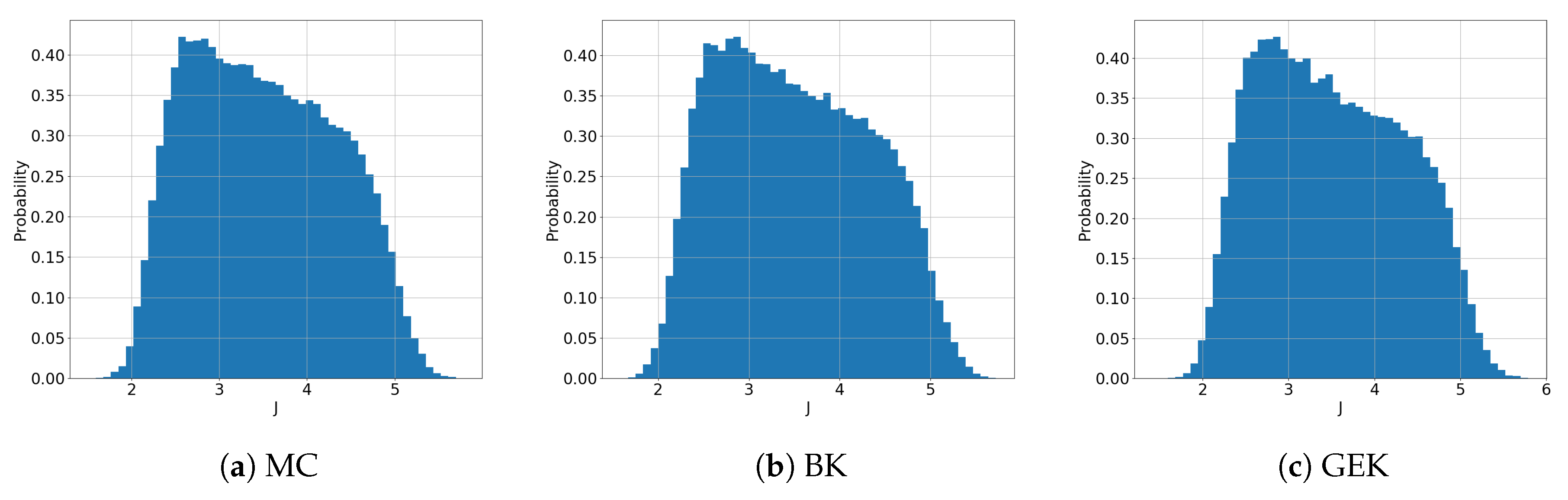
A summary of the UQ results is given in

Table 3. Accuracy and computational efficiency of the UQ solvers.

UQ Method	CFD Solves	Adjoint Solves	$\mathit{E}\left[\mathit{J}\right]$	$\mathit{var}\left[\mathit{J}\right]$	err% $\mathit{E}\left[\mathit{J}\right]$	err % $\mathit{var}\left[\mathit{J}\right]$	Time (s)
MC	1.0 × 10${}^5$	0	3.508	0.6724	-	0.0%	3.0 × 10${}^6$
BK	60	0	3.507	0.6724	−0.03%	0.0%	1.8 × 10${}^3$
GEK (discrete adjoint)	15	15	3.506	0.6724	−0.05%	0.0%	9.0 × 10${}^2$
GEK (continuous adjoint)	15	15	3.467	0.6972	−1.16%	3.69%	6.8 × 10${}^2$
MoM (discrete adjoint)	1	1	3.451	0.6464	−1.63%	−3.87%	6.0 × 10
MoM (continuous adjoint)	1	1	3.451	0.6757	−1.63%	0.49%	4.5 × 10

, where we report the approximated mean and variance of the QoI J according to the various UQ methods. A reference calculation based on MC integration over ${10}^5$ samples is carried out to provide a reference solution. For the present inexpensive test problem, the CPU time required for MC sampling is approximately $3\times {10}^6$ seconds on a personal computer having an Intel(R) Xeon(R) CPU E5-1620 v3 at 3.50 GHz. Results are also reported for MC sampling on the BK surrogate. The latter uses 60 function evaluations at points selected according to a Latin hypercube sampling (LHS) of the six-dimensional uncertain space. The sample size corresponds to the empirical rule $N=10n_{unc}$. This is already sufficient to achieve extremely low errors with respect to the MC mean and variance, while reducing the overall computational cost of the UQ by three orders of magnitude. The GEK UQ based on the discrete adjoint solver provides an accuracy similar to BK by using only 15 samples. Despite the additional adjoint solves for gradient computations, the computational cost is reduced by more than 1/3 with respect to BK. The accuracy of GEK is confirmed by inspection of Figure 3, showing the full empirical pdfs of J computed with PC, BK, and GEK. A very good agreement between MC, BK, and GEK is observed.

The accuracy is less satisfactory for the continuous adjoint approach, due to the less accurate computation of gradients. This reflects numerical errors introduced by the discretization of the adjoint equations and the treatment of boundary conditions, which are not completely consistent with the discretization errors introduced by the direct CFD solver. On the other hand, the continuous adjoint solver is developed independently on the direct solver, and in this sense, it is non-intrusive. The computational cost of GEK samples using the direct or continuous adjoint is approximately the same. The MoM method is obviously less accurate than the other UQ solvers. Nevertheless, the errors on both the computed mean and variance remain very reasonable, despite the presence of a shock in the divergent nozzle(where the Taylor-series expansion is not defined) and the relatively large uncertainty range on the reservoir pressure (approximately 20%). The shock is in practice regularized by numerical diffusion both in the direct and the adjoint solvers, while the uncertainty ranges of all other parameters are reasonably small. While the discrete and continuous-adjoint MoM calculations provide strictly the same results for $E\left[J\right]$ (which does not use gradient information), they predict different results for the standard deviation. The slightly lower errors obtained for the continuous adjoint method is the effect of the compensation of errors for the case at hand. Since the MoM requires only one direct and one adjoint CFD calculation, its computational cost is essentially 1/15 of the GEK sampling. Overall, the first-order MoM provides a reasonably accurate estimate of the lower order statistics of the QoI and a very good tradeoff between cost and accuracy for the present problem. Its accuracy is however expected to decrease for more severe uncertainty ranges. For this reason, the MoM is categorized as a lower fidelity model than BK or GEK.

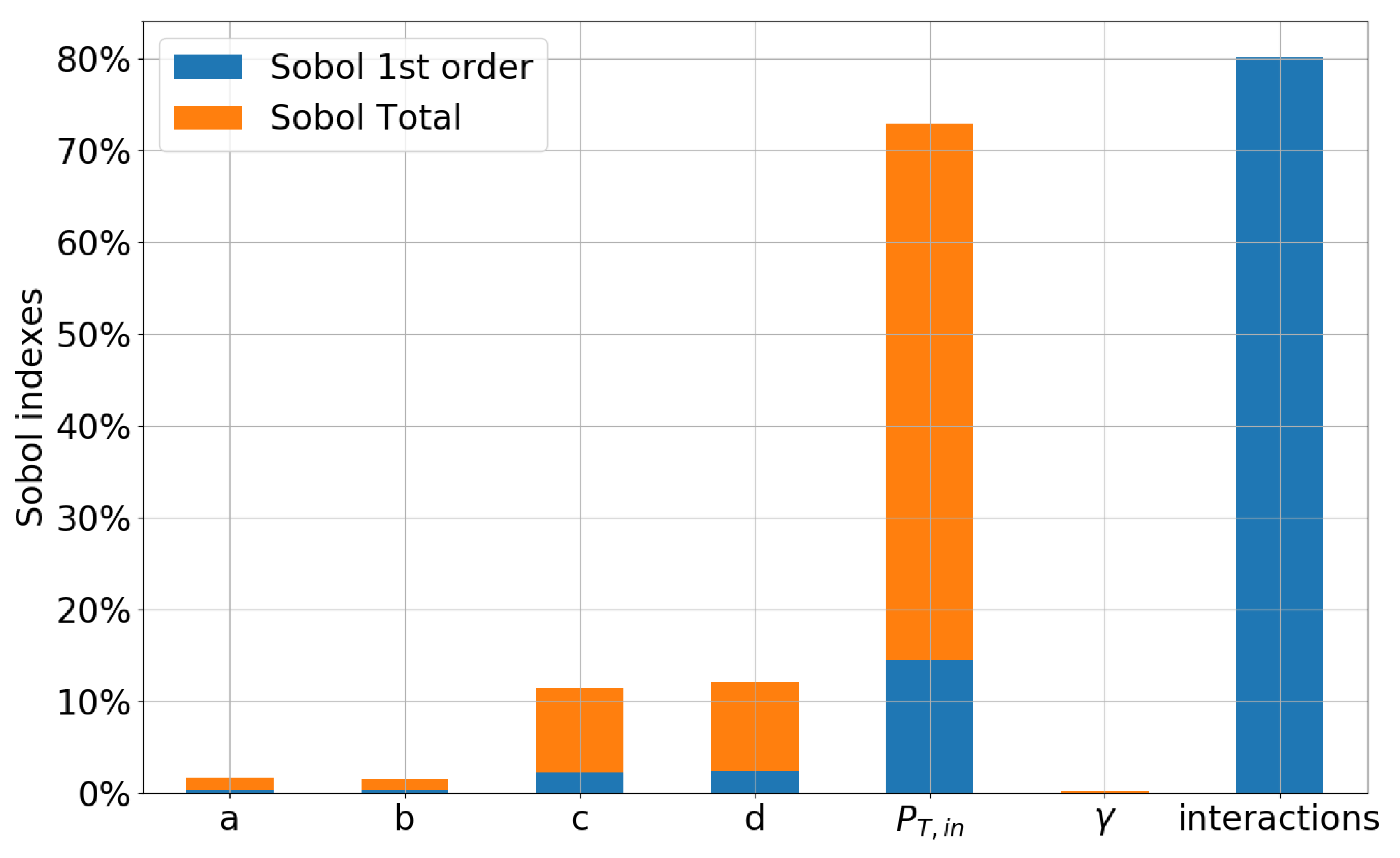
The UQ results for MC, BK, and GEK can be used to carry out a global sensitivity analysis and to identify the random parameters contributing the most to the variance of the QoI by means of an analysis of variance (ANOVA) decomposition. Specifically, exact or surrogate-based MC samples are employed to calculate the Sobol indexes [71] in the parameter space defined by all uncertain inputs. For this purpose, we used the SALib Python library [72]. Only the discrete GEK results (reported in Figure 4) are considered here, the MC, BK, and continuous GEK methods leading to similar conclusions. The figure reports the first-order Sobol indexes with respect to each uncertain parameter, as well as the sum of the higher order indexes, corresponding to the interaction between parameters when these are changed simultaneously. Sobol total indexes are also included in order to further evaluate the relative importance of the various input parameters. The inlet total pressure $P_{T,in}$ appears to be by far the most influential parameter, consistent with the much larger range of its pdf. Nevertheless, the interactions terms are very significant, due to the highly nonlinear nature of the compressible CFD problem, with geometric parameters c and d contributing by more than 10% to the total variance and parameters a and b by more than $2\%$. For this reason, in the RDO calculations of the following section, we treat all six input parameters as random variables.

5.2. RDO Results

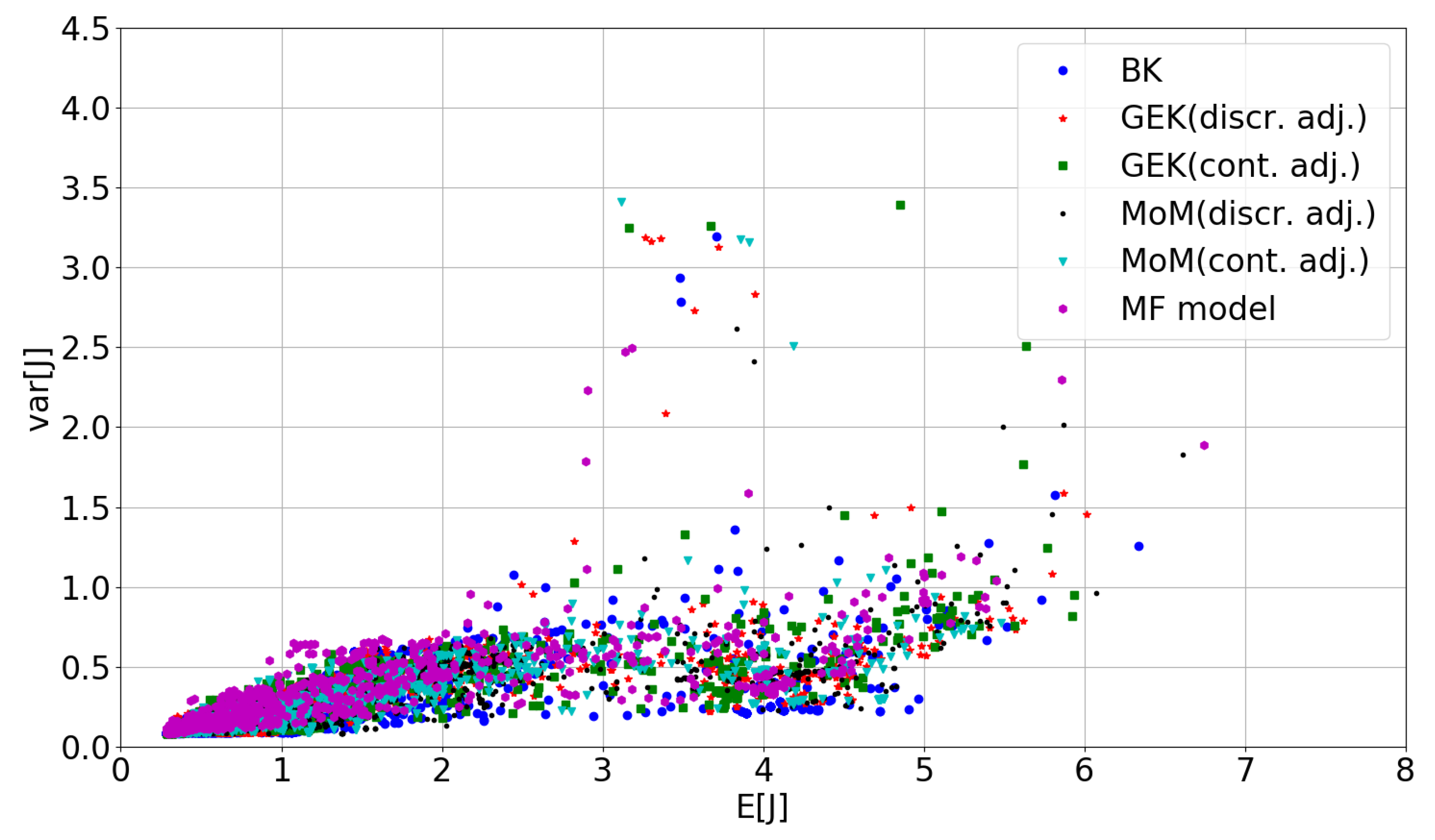
In this section, the UQ methods are coupled with a SMOGA RDO optimizer. The objective is to investigate how different approximations of the statistical models of J, i.e., of the RDO cost functions, may affect the RDO process. The BK and GEK UQ solvers were used in the same setting as Section 5.1, i.e., they are trained for each new design by using 60 and 15 samples in the uncertain space, respectively. This choice provides a good tradeoff between accuracy and computational cost. More sophisticated approaches involving an adaptive refinement of the UQ surrogates are possible and will be the object of future work. Secondly, an MF SMOGA RDO is carried out, and the results are compared with single fidelity RDO. For the single fidelity surrogates, an initial LHS DOE of $10\times n_{des}=40$ UQ runs was carried out prior to the first generation. Then, the first population was randomly initialized in the design space, and the GA was allowed to evolve over 80 generations. MOEI infills were conducted every five generations. For the MF surrogate, the initial DOE contained 40 LF continuous MoM and 10 HF discrete GEK UQ runs. Low-fidelity MOEI infills were added every five generations except for the last infills, for which the tolerance criterion suggested an HF infill. The evolution of the SMOGA search in the objective space $E\left[J\right]\mathrm{vs}.var\left[J\right]$ is depicted in Figure 5 for various RDO optimizers: for each strategy, designs belonging to the first generation, the generations after the first and the second MOEI infill, and the last one are highlighted in red, while all other designs are depicted in grey. For the present inverse design problem, the Pareto front collapses onto a single point corresponding to simultaneous minimization of both objectives $E\left[J\right]$ and $var\left[J\right]$. The progression toward the optimal point is similar for all UQ techniques and optimization surrogates.

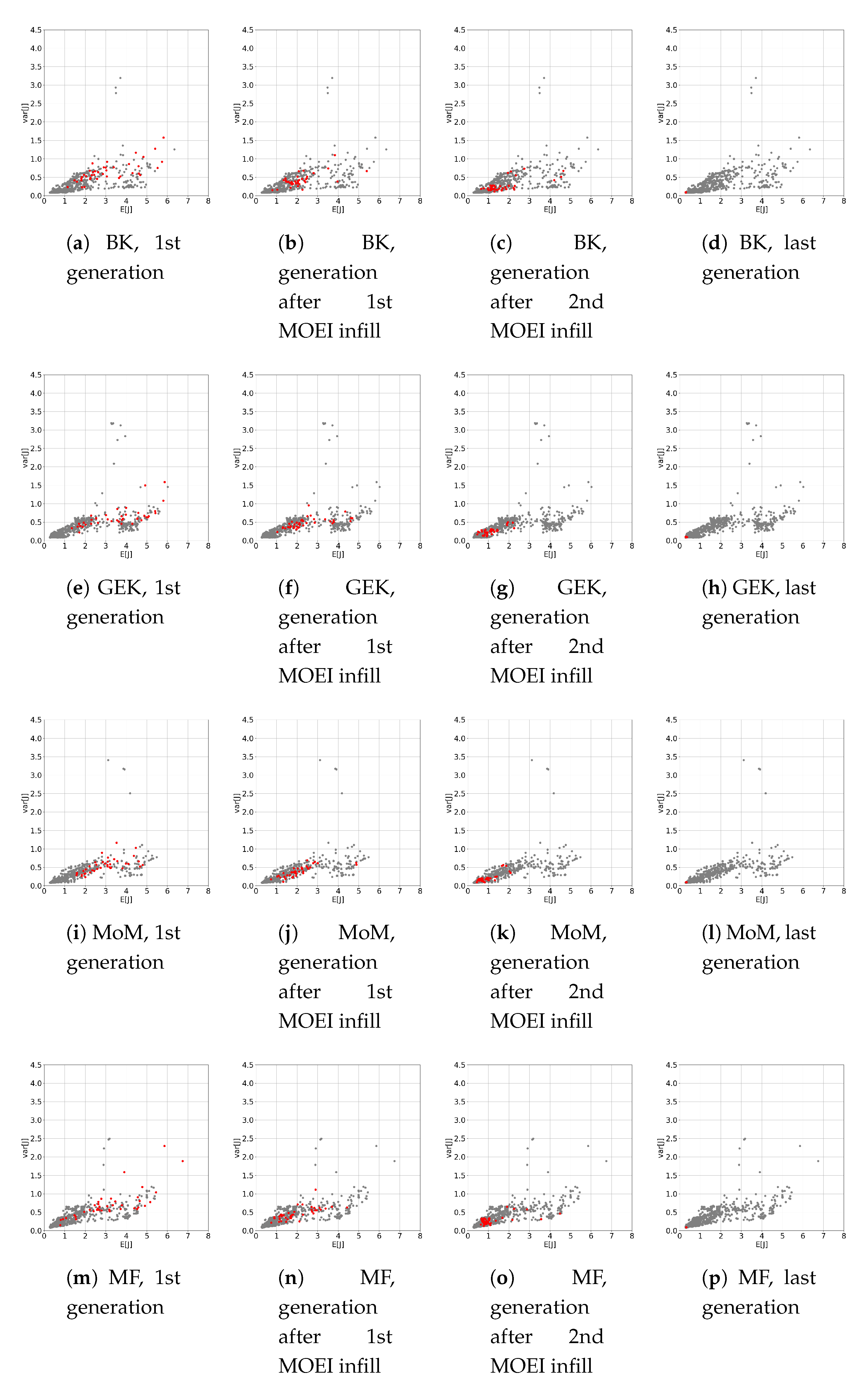
For more clarity, Figure 6 shows the locations of selected GA populations in the objective space. For each technique, four subplots are provided showing in red all points calculated respectively at the SMOGA first generation, at the generation after the first MOEI infill, at the generation after the second MOEI infill, and at the last generation. Moreover, in grey, as a background for each subplot, the reader can find all points calculated with each technique during the SMOGA optimization. It appears that kriging, GEK, the MoM, and MF evolve similarly, as they quickly reach the area near the optimum after only two MOEI infills.

The optimal solutions calculated with each technique are reported in

Table 4. Optimal solutions of RDO according to the various strategies.

UQ Method	E[a]	E[b]	E[c]	E[d]	E[J]	var[J]	Optimization Time (h)
BK	1.500000	0.800000	0.900000	3.900000	0.28509	0.08545	∼20
GEK (discrete adjoint)	1.500002	0.799998	0.900000	3.900000	0.28771	0.08368	∼10
GEK (continuous adjoint)	1.500000	0.799999	0.900000	3.900000	0.28743	0.08416	∼8
MoM (discrete adjoint)	1.500042	0.799961	0.898917	3.940293	0.28514	0.08465	∼0.7
MoM (continuous adjoint)	1.500012	0.799993	0.899999	3.900004	0.28815	0.08502	∼0.5
MF model	1.500000	0.799205	0.899942	3.900006	0.28501	0.08471	∼2.5

. Despite the different accuracy of the UQ techniques in use, all RDO loops converge to very similar solutions identified through the expected values of the four design parameters $[a,b,c,d]$, which differ only on the sixth decimal digit or less for BK, GEK, and MF and on the fifth decimal digit for the MoM. The table also displays the values of the objective functions computed on the surrogate models. BK-BK, GEK-BK, and MF surrogates lead to close estimates of the objective functions, with discrepancies of less than 1% on the mean and less than 2% for the variance. The CPU cost of the different RDO algorithms on a single processor personal computer are reported in the same table. Due to the reduced number of samples used in the UQ runs, the GEK algorithm allows gaining a factor of two to 2.5 over the BK. A further reduction of a factor of 15 or larger is obtained using the MoM, but caution must be taken in systematically preferring such a method for RDO problems, because of its lower accuracy. Finally, the MF SMOGA RDO has a computational time eight times smaller than BK and four times smaller than GEK while ensuring similar accuracy to BK SMOGA.

As a further verification of the RDO results, the optimal design is recomputed using MC sampling, resulting in $E\left[J\right]=0.32325$ and $var\left[J\right]=0.09487$, which is in rather good agreement with the SMOGA estimates, appearing to be slightly over-optimistic in predicting the objective functions. Indeed, the full pdf of the QoI computed by propagating the uncertain parameters through the CFD solution for the optimal nozzle geometry by using the BK and GEK methods (shown in Figure 7 alongside the MC distribution) exhibits moderate deviations from the MC one. Globally, the optimal distributions are much closer to zero on average, and they exhibit a smaller variance than the baseline geometry investigated in the preceding section, showing that the RDO effectively improves both criteria.

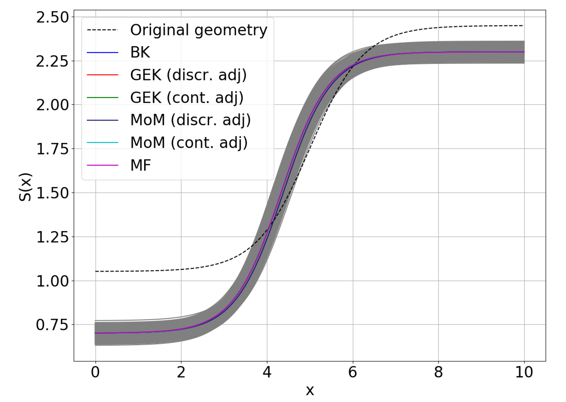
Finally, the optimized geometry is depicted for all of the employed methodologies in Figure 8, and it is compared with the baseline one. The plot is obtained by propagating the pdf of the geometric coefficients through Equation (2), with the mean equal to the optimal RDO values and $CoV=0.01$ as prescribed in Table 4, by using MC sampling. Afterwards, the average geometries and the $3\sigma$ confidence intervals are computed. In the figure, average geometries for all methods are essentially superposed to within plotting accuracy, and the differences are largely smaller than the geometric uncertainty.

6. Conclusions

In the present work, we first assessed various gradient-based methods for uncertainty quantifications, in view of their use for the robust design optimization (RDO) of CFD problems. Specifically, the capability of a Bayesian gradient-enhanced kriging surrogate model and a first-order method of moments to accurately and efficiently compute the lower order statistical moments of a quantity of interest was evaluated for an inexpensive test problem, representative of a supersonic divergent nozzle, for which the results can be compared with well-converged Monte Carlo sampling. The results show that GEK allows computational gains of a factor of two or more with respect to a Bayesian kriging surrogate not using gradient information, when the gradients are efficiently computed using an adjoint method. In the present work, both a discrete and a continuous adjoint method were used for building GEK surrogates. The first one provides more accurate results, but it is somewhat more costly and requires intrusive automatic derivation of the CFD code, which is not possible if, for instance, a commercially available CFD solver is to be employed. The continuous adjoint method allows developing a non-intrusive adjoint solver, but it is less accurate due to inconsistencies in the numerical treatment of the direct and adjoint equations. In the present implementation, the continuous adjoint solver benefits from a direct solution of the linear system of adjoint equations, and it is therefore quicker than the discrete adjoint solver, which converges by means of a pseudo-transient technique. The first-order moment method, based on either discrete or continuous adjoint gradients, is less accurate than GEK, but it still provides satisfactory estimates of the QoI for the present shocked flow problem, due to the relatively small variation ranges of the uncertain parameters.

The UQ methods are then combined with a genetic algorithm for solving the RDO problem. The computations are sped up by constructing a Bayesian kriging surrogate model of the design space. The surrogate is enriched during GA iterations by means of a multi-objective expected improvement (MOEI) infill criterion. For the test problem at hand, the RDO results are found to be similar for the BK, GEK, and MoM methods, the latter being much less expensive in terms of CPU time, but slightly less accurate than the former ones. In order to benefit from the computational efficiency of the MoM and the accuracy of the GEK UQ solvers at the same time, a multi-fidelity surrogate model is built by fusing together the low-fidelity MoM and the high-fidelity GEK. An MOEI infill is used again to enrich the surrogate during convergence, with preference for low-fidelity infills. The multi-fidelity approach successfully identifies the RDO optimum, while dividing by a factor of $3÷4$ the computational cost with respect to GEK. Such an approach is then identified as a promising candidate for more complex RDO problems using CFD models. Further work is however required to assess its effectiveness for more realistic and complex CFD problems. For this aim, its application to the RDO of the stator row of an organic Rankine cycle turbine is underway and will be reported in the near future. In such a context, the introduction of multi-fidelity UQ solvers combining BK and/or GEK based on different numbers of samples could be an interesting future development for further speed up of the RDO procedure.

References

- Beyer, H.G.; Sendhoff, B. Robust optimization—A comprehensive survey. Comput. Methods Appl. Mech. Eng. 2007, 196, 3190–3218. [Google Scholar] [CrossRef]
- Taguchi, G. System of Experimental Design: Engineering Methods to Optimize Quality and Minimize Costs; UNIPUB/Kraus International Publications: Millwood, NY, USA, 1987. [Google Scholar]
- Maliki, M.; Sudret, B.; Bourinet, J.; Guillaume, B. Quantile-based optimization under uncertainties using adaptive Kriging surrogate models. Struct. Multidiscip. Optim. 2016, 54, 1403–1421. [Google Scholar] [CrossRef] [Green Version]
- Razaaly, N.; Persico, G.; Gori, G.; Congedo, P.M. Quantile-based robust optimization of a supersonic nozzle for organic rankine cycle turbines. Appl. Math. Model. 2020, 82, 802–824. [Google Scholar] [CrossRef] [Green Version]
- Cook, L.; Jarrett, J. Horsetail matching: A flexible approach to optimization under uncertainty. Eng. Optim. 2018, 50, 549–567. [Google Scholar] [CrossRef] [Green Version]
- Deb, K. Optimization for Engineering Design—Algorithms and Examples, 2nd ed.; PHI Learning Private Limited: New Delhi, India, 2012; pp. 1–421. [Google Scholar]
- Kochenderfer, M.J.; Wheeler, T.A. Algorithms for Optimization; The MIT Press: Cambridge, MA, USA, 2019. [Google Scholar]
- Congedo, P.; Hercus, S.J.; Cinnella, P.; Corre, C. Efficient robust optimization techniques for uncertain dense gas flows. In Proceedings of the An ECCOMAS Thematic Conference, Antalya, Turkey, 23–25 May 2011. [Google Scholar]
- Bufi, E.A.; Cinnella, P. Robust optimization of supersonic ORC nozzle guide vanes. J. Phys. Conf. Ser. 2017, 821, 012014. [Google Scholar] [CrossRef]
- Cinnella, P.; Bufi, E. Robust optimization using nested Kriging surrogates: Application to supersonic ORC nozzle guide vanes. Ercoftac Bull. 2017, 110, 89. [Google Scholar]
- Congedo, P.M.; Corre, C.; Martinez, J.M. Shape optimization of an airfoil in a BZT flow with multiple-source uncertainties. Comput. Methods Appl. Mech. Eng. 2011, 200, 216–232. [Google Scholar] [CrossRef]
- Cinnella, P.; Hercus, S.J. Robust optimization of dense gas flows under uncertain operating conditions. Comput. Fluids 2010, 39, 1893–1908. [Google Scholar] [CrossRef]
- Congedo, P.; Corre, C.; Martinez, J.M. A simplex-based numerical framework for simple and efficient robust design optimization. Comput. Optim. Appl. 2013, 56, 231–251. [Google Scholar] [CrossRef]
- Hazelton, M.L. Methods of Moments Estimation. In International Encyclopedia of Statistical Science; Lovric, M., Ed.; Springer: Berlin/Heidelberg, Germany, 2011; pp. 816–817. [Google Scholar] [CrossRef]
- Jameson, A.; Martinelli, L.; Pierce, N. Optimum Aerodynamic Design Using the Navier–Stokes Equations. Theor. Comput. Fluid Dyn. 1998, 10, 213–237. [Google Scholar] [CrossRef] [Green Version]
- Giles, M.B.; Pierce, N.A. An Introduction to the Adjoint Approach to Design. Flow Turbul. Combust. 2000, 65, 393–415. [Google Scholar] [CrossRef]
- Cinnella, P.; Pini, M. Hybrid Adjoint-based Robust Optimization Approach for Fluid-Dynamics Problems. In Proceedings of the 54th AIAA/ASME/ASCE/AHS/ASC Structures, Structural Dynamics, and Materials Conference, Boston, MA, USA, 8–11 April 2013. [Google Scholar] [CrossRef]
- Papoutsis-Kiachagias, E.M.; Papadimitriou, D.I.; Giannakoglou, K.C. Robust design in aerodynamics using third-order sensitivity analysis based on discrete adjoint. Application to quasi-1D flows. Int. J. Numer. Methods Fluids 2012, 69, 691–709. [Google Scholar] [CrossRef]
- Papadimitriou, D.I.; Giannakoglou, K.C. Third-order sensitivity analysis for robust aerodynamic design using continuous adjoint. Int. J. Numer. Methods Fluids 2013, 71, 652–670. [Google Scholar] [CrossRef]
- Papadimitriou, D.I.; Papadimitriou, C. Aerodynamic shape optimization for minimum robust drag and lift reliability constraint. Aerosp. Sci. Technol. 2016, 55, 24–33. [Google Scholar] [CrossRef]
- Padulo, M.; Campobasso, S.; Guenov, M.D. Comparative Analysis of Uncertainty Propagation Methods for Robust Engineering Design. In Proceedings of the DS 42: Proceedings of ICED 2007, the 16th International Conference on Engineering Design, Paris, France, 28–31 July 2007; p. DS42_P_158. [Google Scholar]
- Chung, H.S.; Alonso, J.J. Using Gradients to Construct Cokriging Approximation Models for High-Dimensional Design Optimization Problems. In Proceedings of the 40th AIAA Aerospace Sciences Meeting Exhibit, Reno, NV, USA, 14–17 January 2002. [Google Scholar]
- Laurenceau, J.; Sagaut, P. Building Efficient Response Surfaces of Aerodynamic Functions with Kriging and Cokriging. AIAA J. 2008, 46, 498–507. [Google Scholar] [CrossRef] [Green Version]
- Dwight, R.P.; Han, Z.H. Efficient Uncertainty Quantification Using Gradient-Enhanced Kriging. In Proceedings of the 50th AIAA/ASME/ASCE/AHS/ASC Structures, Structural Dynamics, and Materials Conference. American Institute of Aeronautics and Astronautics, Structures, Structural Dynamics, and Materials and Co-located Conferences, Palm Springs, CA, USA, 4–7 May 2009. [Google Scholar] [CrossRef] [Green Version]
- Hercus, S.J.; Cinnella, P. Robust shape optimization of uncertain dense gas flows through a plane turbine cascade. In Proceedings of the ASME-JSME-KSME 2011 Joint Fluids Engineering Conference, American Society of Mechanical Engineers, Hamamatsu, Japan, 24–29 July 2011; pp. 1739–1749. [Google Scholar]
- Cinnella, P.; Congedo, P. Optimal airfoil shapes for viscous transonic flows of Bethe–Zel’dovich–Thompson fluids. Comput. Fluids 2008, 37, 250–264. [Google Scholar] [CrossRef]
- Wang, X.; Hirsch, C.; Liu, Z.; Kang, S.; Lacor, C. Uncertainty-based robust aerodynamic optimization of rotor blades. Int. J. Numer. Methods Eng. 2013, 94, 111–127. [Google Scholar] [CrossRef]
- Peherstorfer, B.; Willcox, K.; Gunzburger, M. Survey of Multifidelity Methods in Uncertainty Propagation, Inference, and Optimization. SIAM Rev. 2018, 60, 550–591. [Google Scholar] [CrossRef]
- Giselle Fernández-Godino, M.; Park, C.; Kim, N.H.; Haftka, R.T. Issues in Deciding Whether to Use Multifidelity Surrogates. AIAA J. 2019, 57, 2039–2054. [Google Scholar] [CrossRef]
- Choi, S.; Alonso, J.; Kroo, I. Multi-Fidelity Design Optimization Studies for Supersonic Jets Using Surrogate Management Frame Method. In Proceedings of the 23rd AIAA Applied Aerodynamics Conference, Toronto, ON, Canada, 6–9 June 2005. [Google Scholar] [CrossRef] [Green Version]
- Parussini, L.; Venturi, D.; Perdikaris, P.; Karniadakis, G. Multi-fidelity Gaussian process regression for prediction of random fields. J. Comput. Phys. 2017, 336, 36–50. [Google Scholar] [CrossRef] [Green Version]
- Kennedy, M.C.; O’Hagan, A. Bayesian calibration of computer models. J. R. Stat. Soc. Ser. Stat. Methodol. 2001, 63, 425–464. [Google Scholar] [CrossRef]
- Shah, H.; Hosder, S.; Koziel, S.; Tesfahunegn, Y.; Leifsson, L. Multi-fidelity robust aerodynamic design optimization under mixed uncertainty. Aerosp. Sci. Technol. 2015, 45, 17–19. [Google Scholar] [CrossRef]
- Forrester, A.I.; Keane, A.J. Recent advances in surrogate-based optimization. Prog. Aerosp. Sci. 2009, 45, 50–79. [Google Scholar] [CrossRef]
- Rozza, G.; Huynh, D.B.P.; Patera, A.T. Reduced Basis Approximation and a Posteriori Error Estimation for Affinely Parametrized Elliptic Coercive Partial Differential Equations. Arch. Comput. Methods Eng. 2008, 15, 229–275. [Google Scholar] [CrossRef] [Green Version]
- Antoulas, A.C.; Beattie, C.A.; Gugercin, S. Interpolatory Model Reduction of Large-Scale Dynamical Systems. In Efficient Modeling and Control of Large-Scale Systems; Mohammadpour, J., Grigoriadis, K.M., Eds.; Springer: Boston, MA, USA, 2010; pp. 3–58. [Google Scholar] [CrossRef]
- Vapnik, V.N. Statistical Learning Theory; Wiley: Hoboken, NJ, USA, 1998. [Google Scholar]
- Ng, L.W.T.; Willcox, K.E. Multifidelity approaches for optimization under uncertainty. Int. J. Numer. Methods Eng. 2014, 100, 746–772. [Google Scholar] [CrossRef] [Green Version]
- Leusink, D.; Alfano, D.; Cinnella, P. Multi-Fidelity Optimization Strategy for the Industrial Aerodynamic Design of Helicopter Rotor Blades. Aerosp. Sci. Technol. 2015, 42, 136–147. [Google Scholar] [CrossRef] [Green Version]
- Fusi, F.; Guardone, A.; Quaranta, G.; Congedo, P. Multifidelity Physics-Based Method for Robust Optimization Applied to a Hovering Rotor Airfoil. AIAA J. 2015, 53, 3448–3465. [Google Scholar] [CrossRef] [Green Version]
- Lewis, R.; Nash, S. A multigrid approach to the optimization of systems governed by differential equations. In Proceedings of the 8th Symposium on Multidisciplinary Analysis and Optimization, Long Beach, CA, USA, 6–8 September 2000. [Google Scholar] [CrossRef]
- Meliani, M.; Bartoli, N.; Lefebvre, T.; Bouhlel, M.A.; Martins, J.; Morlier, J. Multi-fidelity efficient global optimization: Methodology and application to airfoil shape design. In Proceedings of the AIAA Aviation 2019 Forum, Dallas, TX, USA, 17–21 June 2019. [Google Scholar] [CrossRef] [Green Version]
- Forrester, A.I.; Bressloff, N.W.; Keane, A.J. Optimization using surrogate models and partially converged computational fluid dynamics simulations. Proc. R. Soc. Math. Phys. Eng. Sci. 2006, 462, 2177–2204. [Google Scholar] [CrossRef]
- Han, Z.H.; Görtz, S.; Zimmermann, R. Improving variable-fidelity surrogate modeling via gradient-enhanced kriging and a generalized hybrid bridge function. Aerosp. Sci. Technol. 2013, 25, 177–189. [Google Scholar] [CrossRef]
- Zhang, Y.; Kim, N.H.; Park, C.; Haftka, R.T. Multifidelity Surrogate Based on Single Linear Regression. AIAA J. 2018, 56, 4944–4952. [Google Scholar] [CrossRef]
- Forrester, A.I.; Sóbester, A.; Keane, A.J. Multi-fidelity optimization via surrogate modeling. Proc. R. Soc. Math. Phys. Eng. Sci. 2007, 463, 3251–3269. [Google Scholar] [CrossRef]
- March, A.; Willcox, K.; Wang, Q. Gradient-based multifidelity optimisation for aircraft design using Bayesian model calibration. Aeronaut. J. 2011, 115, 729–738. [Google Scholar] [CrossRef] [Green Version]
- Gratiet, L.L.; Cannamela, C. Cokriging-Based Sequential Design Strategies Using Fast Cross-Validation Techniques for Multi-Fidelity Computer Codes. Technometrics 2015, 57, 418–427. [Google Scholar] [CrossRef]
- Park, C.; Haftka, R.T.; Kim, N.H. Remarks on multi-fidelity surrogates. Struct. Multidiscip. Optim. 2017, 55, 1029–1050. [Google Scholar] [CrossRef]
- Gano, S.E.; Renaud, J.E.; Sanders, B. Hybrid Variable Fidelity Optimization by Using a Kriging-Based Scaling Function. AIAA J. 2005, 43, 2422–2433. [Google Scholar] [CrossRef]
- Zheng, J.; Shao, X.; Gao, L.; Jiang, P.; Li, Z. A hybrid variable-fidelity global approximation modeling method combining tuned radial basis function base and kriging correction. J. Eng. Des. 2013, 24, 604–622. [Google Scholar] [CrossRef]
- Fischer, C.C.; Grandhi, R.V.; Beran, P.S. Bayesian Low-Fidelity Correction Approach to Multi-Fidelity Aerospace Design. In Proceedings of the 58th AIAA/ASCE/AHS/ASC Structures, Structural Dynamics, and Materials Conference, Grapevine, TX, USA, 9–13 January 2017. [Google Scholar] [CrossRef]
- Keane, A.J.; Voutchkov, I. Robust design optimization using surrogate models. J. Comput. Des. Eng. 2020, 7, 44–55. [Google Scholar] [CrossRef]
- Serafino, A.; Obert, B.; Hagi, H.; Cinnella, P. Assessment of an Innovative Technique for the Robust Optimization of Organic Rankine Cycles. In Proceedings of the ASME Turbo Expo 2019: Turbomachinery Technical Conference and Exposition, Phoenix, AZ, USA, 17–21 June 2019. [Google Scholar] [CrossRef]
- Loeppky, J.; Socks, J.; Welch, N. Choosing the sample size of a computer experiment. a practical guide. Technometrics 2009, 137, 366–378. [Google Scholar] [CrossRef] [Green Version]
- De Baar, J.H.S.; Dwight, R.P.; Bijl, H. Improvements to Gradient-Enhanced Kriging Using a Bayesian Interpretation. IJUQ 2014, 4, 205–223. [Google Scholar] [CrossRef] [Green Version]
- Le Gratiet, L. Multi-Fidelity Gaussian Process Regression for Computer Experiments. Ph.D. Thesis, Université Paris-Diderot—Paris VII, Paris, France, 2013. [Google Scholar]
- Deb, K.; Pratap, A.; Agarwal, S.; Meyarivan, T. A fast and elitist multiobjective genetic algorithm: NSGA-II. IEEE Trans. Evol. Comput. 2002, 6, 182–197. [Google Scholar] [CrossRef] [Green Version]
- Hirsch, C. Numerical Computation of Internal and External Flows, 2nd ed.; Butterworth-Heinemann: Oxford, UK, 2007. [Google Scholar] [CrossRef]
- Rasmussen, C.E.; Williams, C.K.I. Gaussian Processes for Machine Learning; The MIT Press: Cambridge, UK, 2006. [Google Scholar]
- Wikle, C.K.; Berliner, L.M. A Bayesian tutorial for data assimilation. Phys. Nonlinear Phenom. 2007, 230, 1–16. [Google Scholar] [CrossRef]
- Nelder, J.A.; Mead, R. A Simplex Method for Function Minimization. Comput. J. 1965, 7, 308–313. [Google Scholar] [CrossRef]
- Constantinescu, E.M.; Anitescu, M. Physics-Based Covariance Models for Gaussian Processes with Multiple Outputs. Int. J. Uncertain. Quantif. 2013, 3, 47–71. [Google Scholar] [CrossRef] [Green Version]
- De Baar, J.H.S. Stochastic Surrogates for Measurements and Computer Models of Fluids. Ph.D. Thesis, Delft University of Technology, Delft, The Netherlands, 2014. [Google Scholar]
- Walters, R.; Huyse, L. Uncertainty Analysis for Fluid Mechanics with Applications; NASA Langley Research Center: Hampton, VA, USA, 2002. [Google Scholar]
- Archetti, F.; Candelieri, A. Bayesian Optimization and Data Science; Springer: Berlin, Germany, 2019. [Google Scholar]
- Rojas-Gonzalez, S.; Van Nieuwenhuyse, I. A survey on kriging-based infill algorithms for multiobjective simulation optimization. Comput. Oper. Res. 2020, 116, 104869. [Google Scholar] [CrossRef] [Green Version]
- Močkus, J. On bayesian methods for seeking the extremum. In Optimization Techniques IFIP Technical Conference Novosibirsk, 1–7 July 1974; Marchuk, G.I., Ed.; Springer: Berlin/Heidelberg, Germany, 1975; pp. 400–404. [Google Scholar]
- Dwight, R.; De Baar, J.; Azijli, I. A tutorial on adaptive surrogate modeling. In Introduction to Optimization and Multidisciplinary Design in Aeronautics and Turbomachinery, 7–11 May 2012; Marchuk, G.I., Ed.; Von Karman Institute: Rhode-St-Genèse, Belgium, 2012. [Google Scholar]
- Keane, A.J. Statistical Improvement Criteria for Use in Multiobjective Design Optimization. AIAA J. 2006, 44, 879–891. [Google Scholar] [CrossRef]
- Sobol, I. Global sensitivity indices for nonlinear mathematical models and their Monte Carlo estimates. Math. Comput. Simul. 2001, 55, 271–280. [Google Scholar] [CrossRef]
- Herman, J.; Usher, W. SALib: An open-source Python library for Sensitivity Analysis. J. Open Source Softw. 2017, 2, 97. [Google Scholar] [CrossRef]
- Thévenin, D.; Janiga, G. Optimization and Computational Fluid Dynamics; Springer: Berlin/Heidelberg, Germnay, 2008. [Google Scholar]
- Hascoët, L.; Pascual, V. The Tapenade Automatic Differentiation tool: Principles, Model, and Specification. ACM Trans. Math. Softw. 2013, 39, 1–43. [Google Scholar] [CrossRef] [Green Version]
Figure 1.
Baseline quasi-1D nozzle.
Figure 2.
Flowchart of the BK-based SMOGA RDO process.
Figure 3.
Assessment of UQ methods: approximate pdf of QoI J for MC, BK, and GEK.
Figure 4.
Global sensitivity analysis with Sobol indexes.
Figure 5.
Objective space.
Figure 6.
Evolution of the convergence for BK, GEK, MoM, and MF. Red color highlights designs belonging to the first generation, generations after the first and the second MOEI infill, and the last one. Other designs are in grey color.
Figure 7.
pdf of the QoI J for the optimal solutions in Table 4.
Figure 8.
Baseline geometry and optimized geometries (with uncertainty intervals) for various RDO strategies.