Exploring the Dynamic Organization of Random and Evolved Boolean Networks


1
Department of Physics, Informatics and Mathematics, University of Modena and Reggio Emilia, via Campi 213a, 41125 Modena, Italy
2
Institute for Advanced Study, University of Amsterdam, 1012 WX Amsterdam, The Netherlands
3
European Centre for Living Technology, 30123 Venezia VE, Italy
*
Author to whom correspondence should be addressed.
Algorithms 2020, 13(11), 272; https://0-doi-org.brum.beds.ac.uk/10.3390/a13110272
Submission received: 27 August 2020
/
Revised: 19 October 2020
/
Accepted: 26 October 2020
/
Published: 28 October 2020
(This article belongs to the Special Issue Artificial Cognitive and Evolutionary Systems)
Abstract
:The properties of most systems composed of many interacting elements are neither determined by the topology of the interaction network alone, nor by the dynamical laws in isolation. Rather, they are the outcome of the interplay between topology and dynamics. In this paper, we consider four different types of systems with critical dynamic regime and with increasingly complex dynamical organization (loosely defined as the emergent property of the interactions between topology and dynamics) and analyze them from a structural and dynamic point of view. A first noteworthy result, previously hypothesized but never quantified so far, is that the topology per se induces a notable increase in dynamic organization. A second observation is that evolution does not change dramatically the size distribution of the present dynamic groups, so it seems that it keeps track of the already present organization induced by the topology. Finally, and similarly to what happens in other applications of evolutionary algorithms, the types of dynamic changes strongly depend upon the used fitness function.
1. Introduction
Many natural, social or artificial systems can be described as networks of interacting elements, where the dynamical variables are associated to the nodes of the network, and directed links represent the influence of a variable upon another one. While networks can represent different kinds of systems and relationships, let us consider here for the sake of definiteness a dynamical system. A variable xi(t) (i = 1…N), which can take either continuous or discrete values, is associated to every node i of the network at time t, and a deterministic law (e.g., a differential or finite difference equation) determines the time behavior of xi. If this equation contains at least one term which depends upon xj then there is a link from node j to node i.
The study of the properties of networks has become one of the major threads in complexity science. The discovery of the widespread presence of some types of topological relationships, associated to important generic properties (like e.g., the presence of hubs), prompted several studies on topology [1,2,3]. It soon became clear that the properties of these complex systems are neither determined by the topology of the interaction network alone, nor by the dynamical laws in isolation, but they are the outcome of the interplay between topology and dynamics [4,5,6,7,8,9]. This implies that it is difficult to tell in advance what the properties of a complex system are, unless of course it belongs to a class of already well-studied cases.
We will loosely use the term “dynamical organization” to refer to the emergent properties of the interactions between topology and dynamics. It goes without saying that there may be different organizational levels, and that in general a simple hierarchical scheme may not be adequate. Different methods to explore the dynamical organization of complex systems can be proposed. In this paper, we make use of one such method, which was introduced by us some years ago [10,11] and which has later been improved [12] and applied to different classes of systems [13,14,15,16]. The method identifies integrated groups of variables, by means of measures based upon information theory (the Relevance Index methodology—RI in the following), which is briefly recalled in Section 2.1 (referring the interested reader to the literature [12] for further details).
In this paper, we concentrate on an important class of models, i.e., the so-called random Boolean networks (RBNs) which were initially conceived by Kauffman as a simplified model of genetic regulatory networks, and which turned out to be one of the most general and most widely used models in the field of Complex Systems Science. The definition and properties of RBNs are briefly reviewed in Section 2.2.
Due to their randomness, the study of single RBNs makes little sense, and it is necessary to study the behavior of families of networks, built at random while keeping some parameters fixed—in a way which closely parallels the ensemble approach of statistical mechanics [17,18,19]. A very important feature of families of RBNs is that their “typical” behaviors can be ordered or disordered, depending upon the value of some parameter. This makes them well-suited to study the transitions between order and chaos and, for this reason, they have been analyzed in-depth by several groups [20].
It can indeed be shown that a single parameter, the so-called Derrida parameter λ (which is sometimes called the dynamical sensitivity) distinguishes between ordered (λ < 1) and disordered (λ > 1) systems. In ordered systems, a slight perturbation of the initial conditions tends to die out, while in chaotic networks it initially increases. In so-called critical systems, i.e., those which are neither ordered nor chaotic (λ ≅ 1), a small perturbation tends on average to keep the same size unaltered.
Particular attention has been devoted to these critical RBNs, since it has been suggested that they might achieve an optimal tradeoff between the need to be robust with respect to some external changes and the capacity to react to other external changes—a key property for living systems and for autonomous robots. Moreover, critical networks might be better evolvable than ordered and chaotic ones. Note also that the importance of criticality may well go beyond the boundaries of RBNs: indeed, the criticality hypothesis, i.e., the idea that dynamically critical states possess some peculiar advantages, so that they tend to be selected under evolutionary dynamics [21,22,23,24,25,26,27,28,29,30,31], can hold for a much wider class of dynamical models, including the dynamics of the biological neural networks [32] or the behavior of artificial systems [33]. These very important aspects are major research topics and they cannot be discussed here in detail, so we refer the interested reader to some recent papers [27,33]. For the sake of definiteness, this paper concentrates indeed on the features of the dynamical organization of critical RBNs.
As will be briefly recalled in Section 2.2, RBNs are indeed really random: the connections between the nodes are drawn at random, and so are the Boolean functions which determine the new state (at time t + 1) of a node, from the values of its input nodes at time t. Very little “organization” can be expected here. Yet, we show below that the existence of dynamically integrated groups of nodes in a network can be inferred from an analysis of the perturbations of gene expression levels (“avalanches”), induced by a permanent clamping of a node to a fixed value. As anticipated above, the identification of such integrated groups of nodes can be performed by means of the RI methodology described in Section 2.2. The fact that dynamical integration actually takes place is demonstrated by comparing the dynamically relevant groups, which are detected by simulating actual RBNs with those that are found in “fully random” avalanches, generated at random with the same size distribution (avalanches are also described in Section 2.2). The comparison of the size distribution of integrated groups of nodes in avalanches in RBNs with the size distribution of integrated groups of nodes in fully random avalanches is described in Section 3.1. As it will be stressed in the conclusions (Section 4), the two distributions are markedly different, thus showing that the sharing of a common topology induces significant correlations among the nodes—which cannot of course be observed in purely random avalanches. To the best of our knowledge, this is the first case where this kind of (dynamical) organization in truly random BNs has actually been detected.
Given the importance of critical RBNs, we have also introduced an evolutionary algorithm which ensures that a population of critical Boolean networks remains critical during its evolution. Starting from purely random Boolean networks, the population evolves according to a Genetic Algorithm (GA) in order to maximize a given fitness function; for example, the achievement of attractors with a predefined fraction of active genes. A standard GA easily performs this task by changing the bias of the set of Boolean functions (see Section 2.2 for a definition of the bias) but, in doing so, it leads the networks in the ordered region. Thus, if criticality can provide some other advantages, these are lost in evolution. We have therefore introduced a modified GA which tends to keep the evolved networks critical. It has been presented elsewhere [34], where we have also shown that it is successful in maintaining criticality while achieving its goal, in the case where the goal is a fixed fraction of active nodes (as in the example just discussed), as well as in the case where the target is that of giving rise to avalanches with a predefined fraction of “up” nodes, i.e., nodes whose activation is higher in the perturbed network than in the wild type. The modified GA is briefly recalled in Section 2.3.
Since the RI methodology has been successful in showing some organization of fully random Boolean networks, we have decided to apply it to also study the differences between RBNs and the populations of evolved networks in the two cases above. Note that the evolved networks are no longer fully random, although they are dynamically critical. As will be shown in Section 3.2, the method proves able to identify measurable differences between the RBNs and the evolved networks, thus showing its capacity to react to this form of organization. Similarly to what happens in other applications of evolutionary algorithms to RBNs, the types of changes strongly depend upon the fitness function, as briefly discussed in the final Section 4.
2. Materials and Methods
2.1. The Relevance Index
The Relevance Index (RI) methodology, which draws its inspiration from methods used in neuroscience [35,36], makes use of indexes based on information theory and is suitable for exploring the organization of complex systems. In particular, we utilize the index called zI (see below), which makes it possible to identify, as components of a system, sets of variables that show a high degree of internal coordination. The RI methodology has been applied with interesting results to several systems: some of them had been artificially designed in order to test the effectiveness of the technique, while others referred to interesting physical, chemical, biological, or socio-economic systems [13,14,15,16].
Let U be the set of discrete variables {x1, x2… xn} describing a system whose status changes along a collections of m observations, and a subset S of U composed of k elements. Its integration I(S), semidefinite positive, is defined as:
where H represents the Shannon entropy (respectively, of the involved variables and of the subset as a whole). The integration of a (sub)set of variables could be interpreted as their distance from the independence condition [35]—the greater the distance, the greater the probability that the variables of interest are exchanging information. We can note that the number of variables that can be correlated is arbitrary (obviously, there are limits to this “arbitrariness”: for further details, see [35]): in particular, the use of integration allows to (a) overcome the pairwise analysis (a group of four elements is not always the simple merge of six binary interactions) and (b) to highlight some kinds of nonlinear relationships otherwise not visible [11,35].
The integration depends on the size of the group under observation and the size of the alphabet of the elements that compose it (elements that determine the number of degrees of freedom of the system) and on the number m of observations: in order to rank the examined groups, therefore, we need to normalize the integration according to these terms. A useful formula could be found in [12]:
where we insert within a z-score form the information that the integration multiplied twice by the number of observations follows a Chi-square distribution with d freedom degree:
the Lj terms denoting the cardinality of the alphabet of the j-th variable belonging to the subset S to be analyzed.
Ideally all possible groups have to be tested and sorted in descending order with respect to the zI index: the independent non overlapping groups that survive a sieve action are the potentially Relevant Sets (RSs in the following) [12]. All the first RSs in the list are then selected to be collectively represented by single variables, which are introduced in place of the original ones to form a new data series: the cycle of analysis, sieving, and compacting repeats several times until the last computed zI index reaches a minimum threshold (the number of all possible subsets of a set grows indeed very rapidly: it is, however, possible to sample the subsets to be tested in various ways (including the use of optimization strategies) [37,38], while the combination of the compaction and iteration procedures helps in allowing the identification of large groups [12]). The z-score typically has the purpose of verifying whether the mean value of a distribution deviates significantly from a certain reference value: in this paper, we will assume as reference thresholds θ3 = 3.0 and θ5 = 5.0, which in the case of Gaussian statistics correspond, respectively, to p-values close to 1.3⋅10−3 and 2.7⋅10−7.
At the end of the analysis, groups of variables of different sizes (and possibly single not aggregated variables) are obtained. This grouping is based on the observation of the behavior of the (single and collective) variables along the observations: its characteristics, therefore, depend on the system’s dynamics.
2.2. Random Boolean Networks
Random Boolean Networks are a well-known model of gene regulatory dynamics [17,18,19,20,24,30,39,40,41] able to perform computation [42]. In this section, we present a synthetic description of the RBN model, referring the reader to [17,18,20,23,24] for more details. Several variants of the model have been presented and discussed [43,44,45,46], but we will restrict our attention here to the “classical” model.
A RBN, as introduced by Kauffman [23,24,39], is a dynamic system whose components (nodes in an oriented graph, each one representing a gene of a genetic regulatory network) can assume only two levels (0 and 1). If the state of a single node can be represented by xi(t), the state of the whole network can be represented by the vector X(t) = [x1(t), x2(t), … xN(t)]. In “classic” RBNs, each node has the same incoming connectivity, while multiple connections and auto-connections are prohibited. Each node is associated with a Boolean function, which represents the response to the signals (proteins—not represented in the model) coming from the upstream nodes. In this paper, in case of random generation of the Boolean functions, for each entry, we extract a 1 with probability p (a quantity called “bias”)—and consequently the frequency of the values equal to 0 is (p − 1).
The topology and Boolean function associated to each node do not change in time, and the network dynamics is discrete and synchronous, so fixed points and cycles are the only possible asymptotic states in finite networks.
The RBN’s average degree of connectivity and the type of Boolean functions influence the behavior of the system, which can show ordered or disordered dynamic regimes. In ordered regimes, there are few attractors, whose period scales as a power law with the number of nodes N of the system, while in disordered regimes, the period of the very numerous attractors scales as a more than polynomial function [23,24]. The disordered regime also shows a strong sensitivity to initial conditions, which is not present for the ordered regime.
As mentioned in Section 1, these different behaviors can be related to the value of a single index, often called the Derrida parameter λ: on average, a small perturbation tends to vanish in “ordered” networks (λ < 1), while in chaotic networks (λ > 1) it increases in time, and in critical networks (λ = 1) it tends to maintain its size. The Derrida parameter can be determined by studying the average behavior in time of the distance between two close initial states of a network and taking its limiting value when the initial distance approaches its minimum value (dynamical sensitivity) [20,47,48]. However, direct measurement of the dynamical Derrida parameter in physical biological systems may be prohibitive, due to their transient nature, but it is sometimes possible, under plausible assumptions, to circumvent this problem and to infer the value of λ from other data. This is the case of the effects of gene perturbations, induced by permanently inhibiting the expression of a single gene (knock-out) and by observing the changes of the expression levels of the other genes.
In synthetic networks (by means of simulations), it is possible to evaluate these effects by comparing the behavior of a non-perturbed system (“wild type”, briefly WT) with the behavior of a perturbed system, which differs from the previous one in that one of the genes, which are active in the WT system, is silenced (its Boolean function is fixed at False—“knock-out” event). It is possible to observe the two systems over time, and to mark nodes having different values in the different systems as “perturbed” nodes: the number of such nodes (different from the silenced node) provides the size of the “avalanche of changes” (or more briefly “avalanche”) to which these nodes belong. In order to avoid the idiosyncrasies of single networks, each perturbation is carried out on a different RBN belonging to the same statistical “ensemble” (same number of nodes N and same bias p). Avalanches are important in this study because they constitute the experimental observations from which some aspects of the dynamic organization of systems subject to perturbation can be deduced [40].
2.3. Genetic Algorithm
In this paper, we are interested in highlighting the presence of significant dynamic structures in dynamic systems, and in observing the changes in their characteristics passing from random systems, to systems with organization, up to evolved systems—in our case, evolved by means of Genetic Algorithms (GA in the following) [49].
It should be noted that in this article, we make use of genetic algorithms in a twofold way, since we are interested in their ability (a) to solve problems, and (b) to emulate evolution.
Indeed, evolutionary and in general bio-inspired algorithms—based on the principles of the biological evolution [49,50], or on the self-organized behavior of some groups of animals such as colonies of ants, flocks of birds, and schools of fish [51,52,53,54]—play a fundamental role in complex optimization problems, allowing the development of new and robust techniques. These techniques show characteristics such as adaptation, scalability, speed, autonomy, parallelism, and fault tolerance. As consequence, several algorithms inspired by evolution [55,56] or biological behaviors of groups of animals [52,57,58,59] have been used to find near-optimal solution to complex optimization problems in several areas. Alongside these by now “classic” themes, in recent years, there has been an interesting increase in the variety of bio-inspired algorithms, inspired by the success of plant lifestyles [60,61], by some flight behaviours [62] or hunting behaviours in mammals [63,64,65,66], or by the presence of hierarchies [67] and opportunistic behaviours [68] in birds. Very often, this type of algorithms turns out to be the best option when an exact optimizer would not be able to give results in admissible times [55]. Bio-inspired meta-heuristic optimization algorithms are turning out to be increasingly used in different applications since they are: (i) based on simple ideas, easily implemented; (ii) typically not strongly dependent on the structure of the optimization problem; (iii) able to find a near-optimal solution; and (iv) easily applicable in different areas [52]. In this context, the GA framework plays a significant role [50].
On the other hand, for our aims, the GA’s ability to mimic the natural evolutive processes [49,69] is also very interesting.
Because of the evolution, the final populations are no longer random as in the beginning—although they still preserve some randomness—so in the following, we will indicate them with the term “BN”, where the character “R” for “random” has been removed.
The initial populations on which the GA acts are composed by RBNs sharing the same topology, the genotype of each individual being composed of the sequence of the truth tables of the Boolean functions that guide the dynamic response of each individual’s node. Due to the arbitrariness of the numbering of nodes, the fixed topology does not limit the set of networks that can be generated. We run a series of experiments with networks whose nodes have two inputs each, the first generation being composed of random systems having the Boolean function bias equal to 0.5—and therefore typically showing a critical dynamic regime (see the previous section).
Given that criticality is supposed to be an important property, it is particularly interesting to consider a modified version of the GA, presented in [34], which preserves the bias of the Boolean functions during inheritance from parents to children. This GA maintains the usual selection procedure (a roulette wheel) and has a slightly modified mutation and crossover. In particular, we use the single-point crossover (where the cut-off point is randomly chosen among those that keep the parental bias as much as possible), while the mutation hits randomly, but in a way to again get closer to the bias of the parents. It has been verified that this modified GA preserves the bias of the initial individuals: additionally, in case of populations composed of dynamically critical individuals, the property of criticality is maintained over the generations [34]. (In this article, we follow the classic criticality measure for RBNs, represented by the Derrida procedure carried out on a high number of random initial conditions [20,47].)
By following this approach presented in [12], we aim to obtain two populations of BNs, evolved with two different purposes: in one case, we search for the highest possible number of active nodes on attractors (a non-trivial task, wanting to keep the BNs in critical regime—Fit1 in the following), while in the other, we want avalanches following knock-out events to be composed of nodes whose response to stress is more of an increase than a decrease in activity (Fit2 in the following), a feature present in knock-out events in living systems [70]. (In particular: Fit1 identifies the system attractors, computes the average value of each node among each attractor, and computes the fitness function as the fraction of average values greater than 0.5; Fit2 reaches a random chosen attractor, computes the average value of each node among the attractor, and performs knock-out events on nodes having positive averages, recording the fraction of nodes (downstream from the silenced ones) that present an increase in activity with respect their state in the unperturbed situation: the fraction is the fitness value. See [12] for more details.)
As already commented, in each GA run, the population of BN is made up of networks sharing the same topology, the genotype being composed by the sequence of Boolean functions that determine the dynamic response of each node. (Due to the arbitrariness of the position of nodes, the fixed topology does not limit the set of networks that can be generated.) For each fitness, we made 50 GA runs; Table 1 presents the parameter values used during simulations. (In the cases we analyzed, 100 generations were enough to reach a maximum fitness that could not be further improved, while the increase in average fitness also stopped. We made some sample of runs even considerably longer, without observing substantial changes.)
3. Results
3.1. Random Avalanches and Avalanches in Random Boolean Networks
A well-known technique in the study of gene regulation is that of inducing a permanent clamping of the activation value of a gene to a fixed value, e.g., by silencing it (knock-out events) [70]. The genes involved in each avalanche can react to the perturbation by increasing or decreasing their activity, situations identified later in the article by the terms UP and DOWN.
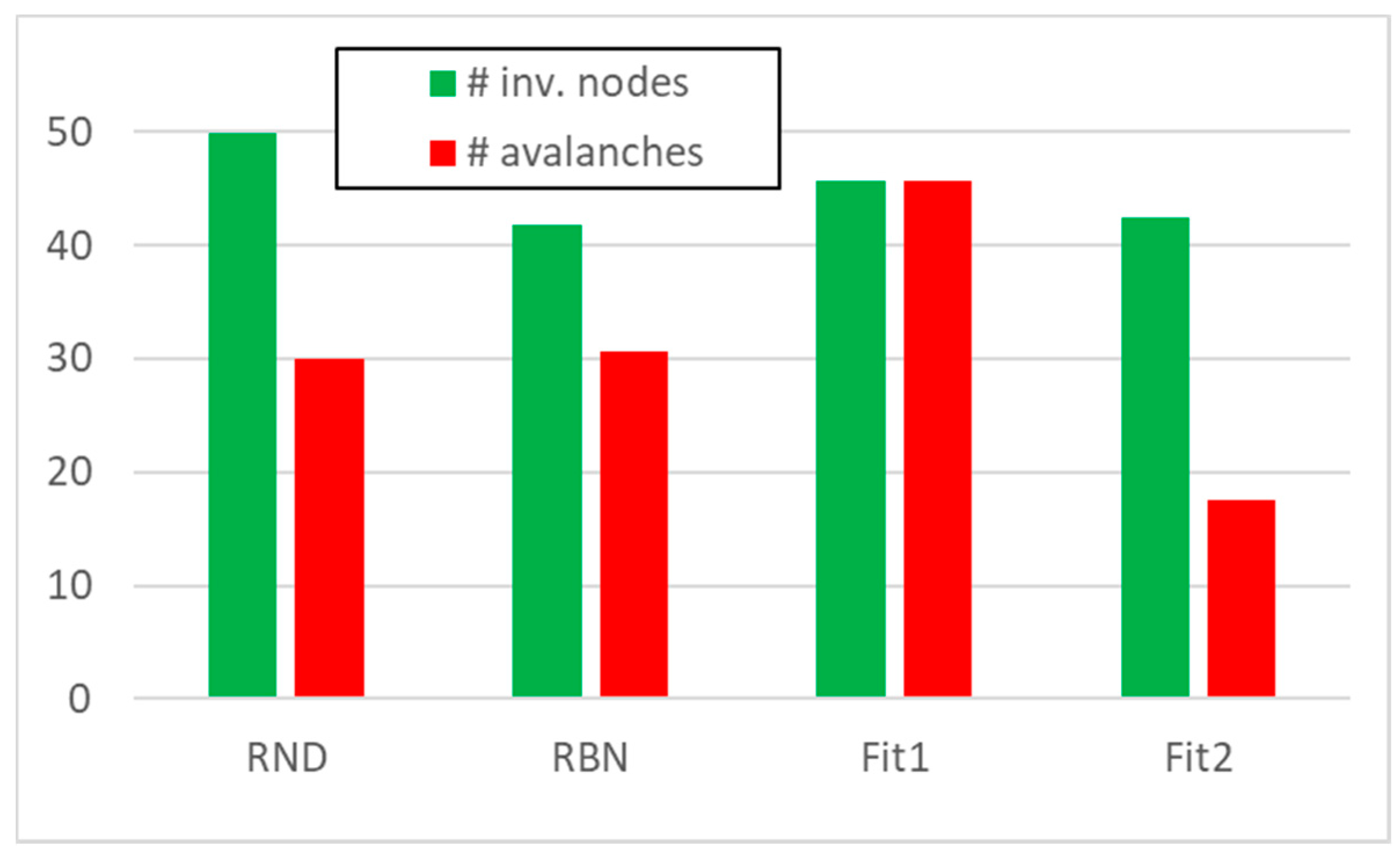
We then performed knock-out experiments in 50 RBNs each composed by 50 nodes—following an approach already developed in [12]—blocking to zero, one at a time, each node whose average activity on the attractor was greater than 0.5. In each of the analyzed systems, we obtained from 18 to a maximum of 45 avalanches, with an average on the total of 50 RBNs very close to 30 avalanches; in doing this in each system on average, about 40 nodes were affected by at least one avalanche (Figure 1, “RBN” system class). (For presentation convenience, in the following, we will use the term “RBN” to indicate in general the framework of the Random Boolean Networks, to indicate a system “class” (the particular collection of RBNs we use in this paper), and to indicate a single exponent belonging to the aforementioned class. In the rare case of ambiguity, we will explicitly manage the different situations.)
We then created 50 groups of avalanches, each group being composed by 30 avalanches with a size distribution like the one found in the 50 RBNs; each node belonging to an avalanche can have UP or DOWN value with equal probability (the typical situation for RBNs). In these random avalanche groups, typically all nodes were affected by at least one avalanche (Figure 1, “RND” system class). (Let us discuss first the results regarding these first classes of systems, by leaving to next sessions the introduction and discussion of the two classes of evolved systems (indicated as Fit1 and Fit2 in Figure 1.))
In each RBN (and in each group of the RND class) the nodes constitute the variables to be grouped, depending on their behavior in the m observations, each observation being a complete measure of response to the initial perturbation, that is, an avalanche. The final distribution of the groups identified by the RI analysis based on the index zI (i.e., the final RSs) provides us with clues about the dynamic organization of each system—that is, how the nodes form dynamically integrated groups, influencing in such a way the progress of the perturbations.
We can perform the RI analysis by using in succession the two previously introduced threshold levels: in the case of the θ5 threshold, we are focusing our attention on the most dynamically active elements, while the θ3 threshold has so far been used as a level below which it is no longer correct to carry out mergers (create larger collective variables) [12].
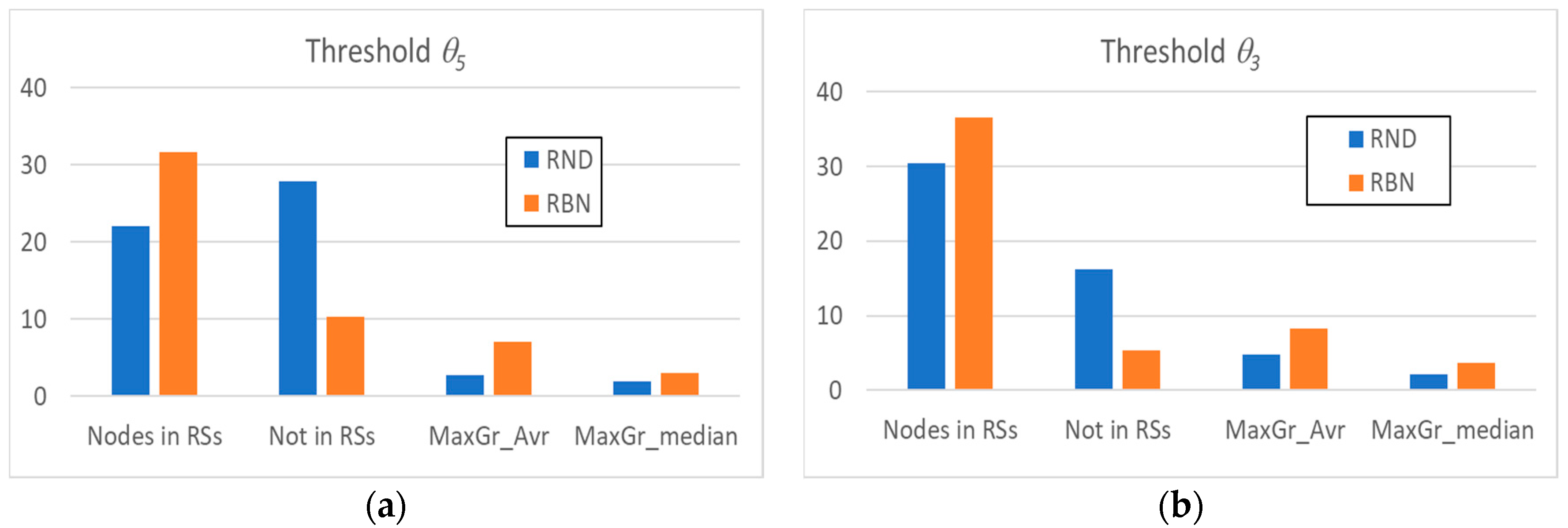
Figure 2a shows some of the main average characteristics of the obtained RSs’ distributions by using the θ5 threshold. We can note that, despite the fact that the avalanches in RND systems involve a very high number of nodes, the nodes present within a RS are significantly less than the nodes present within a RS in RBN systems.
In other words, in RND systems, most of the nodes show absence of correlation with other nodes (a clue indicating absence of dynamic organization). Furthermore, it is possible that some group of nodes is present by chance, but their sizes compared to those of the groups in RBN systems are extremely limited, as evidenced by the comparison between the average size of the maximum and median RS of the two system classes.
The same observations can be made by analyzing the systems with the θ3 threshold (Figure 2b), with the obvious remark that the total number of nodes belonging to at least one RS increases; the average and median RSs’ sizes also increase, but the ordering between the classes remains unchanged. The same holds in all our experiments: therefore, for the sake of simplicity, in the following, we will always use the θ5 threshold.
As a final comment of this section, we can note that the propagation of perturbations in random systems is considerably different from having perturbations themselves random: the introduction of a topology—even if it is itself random—introduces an strong element of dynamic organization.
3.2. Static and Dynamic Characteristics in Evolved Systems
The evolved systems present a dynamic organization that is certainly different from that present in random systems. Interestingly, this difference is not always evident using structural analyses alone.
A first difference with respect to random system with structure (the RBN class) can be seen in Figure 1 (Section 3): the increased number of genes active on attractors in systems evolved with Fit1 fitness allows a higher number of knock-out events; nevertheless, the increase in the number of nodes involved in avalanches does not increase in proportion. On the contrary, systems evolved with Fit2 fitness present very few nodes susceptible of knock-out events. These differences in external behavior, however, do not provide clues to identify the internal dynamic organization of these systems.
Remember that all individuals of each GA run share the same initial random topology: thus, the action of the GA involves frequency distribution of the Boolean functions, and/or the adjacency map of all the possible pairs of Boolean functions.
Each of the 16 Boolean functions has 50 chances of appearing in an RBN, and in each group, there are 50 RBNs: indeed, out of the 2500 potentially possible presences, each Boolean function appears less than 250 times. To verify the distance from a uniform distribution situation (156 presences for each Boolean function), it is therefore possible to apply the Chi-square test [71].
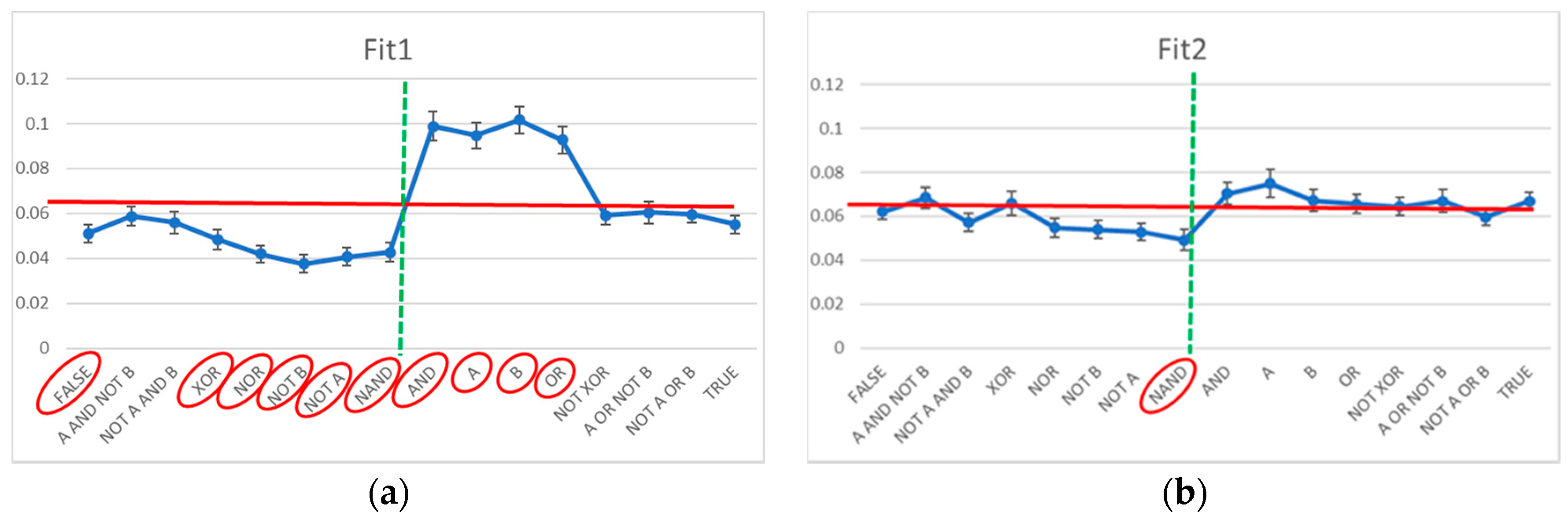
The Chi-square test indicates that the distribution of the Boolean functions in the case of Fit1 systems is significantly anomalous (a values of 286 vs. a significance threshold of 25): by analyzing the observed frequency of each Boolean function vs. the expected ones (in case of uniform random distribution), 10 out of 16 functions show a significant deviation at the level of 1% (Figure 3a). The Chi-square test conducted on the Boolean function adjacency matrix (given the observed frequencies of each Boolean function) highlights a further deviation (a value of 513 vs. a significance threshold of 291). The frequencies of the pairs of Boolean functions deviate strongly from the expected ones: that is, the dynamical organization of the system derives from an adjustment of both the frequencies of the Boolean functions and their linking. In Figure 3a, the Boolean functions of Fit1 systems are in order by final bit, so as to highlight the decrease in frequency of the functions having a “0” output in correspondence with an input “1,1”, and an increase in the functions having a “1” output in the same case. This observation is compatible with the fact that the asymptotic states of these systems must have a high number of active genes. (This observation is compatible with a remark present in [34], albeit this latter remark provides a lower evidence because of the smaller number of analyzed systems.)
The results are markedly different in the case of Fit2 systems. The Chi-square test indicates that the distribution of the Boolean functions is only slightly anomalous (a values of 31 vs. a significance threshold of 25): by analyzing the observed frequency of each Boolean function vs. those predicted in case of random uniform distribution, only 1 out of 16 functions show a significant deviation at the level of 1% (Figure 3b). The Chi-square test conducted on the Boolean function adjacency matrix (given the observed frequencies of each Boolean function) does not evidence deviations (a value of 269 vs. a significance threshold of 291). That is, the static analysis does not evidence almost any significant modification with respect to a random organization.
Interestingly, a more direct observation of the dynamic organization highlights some characteristics of the systems under investigation.
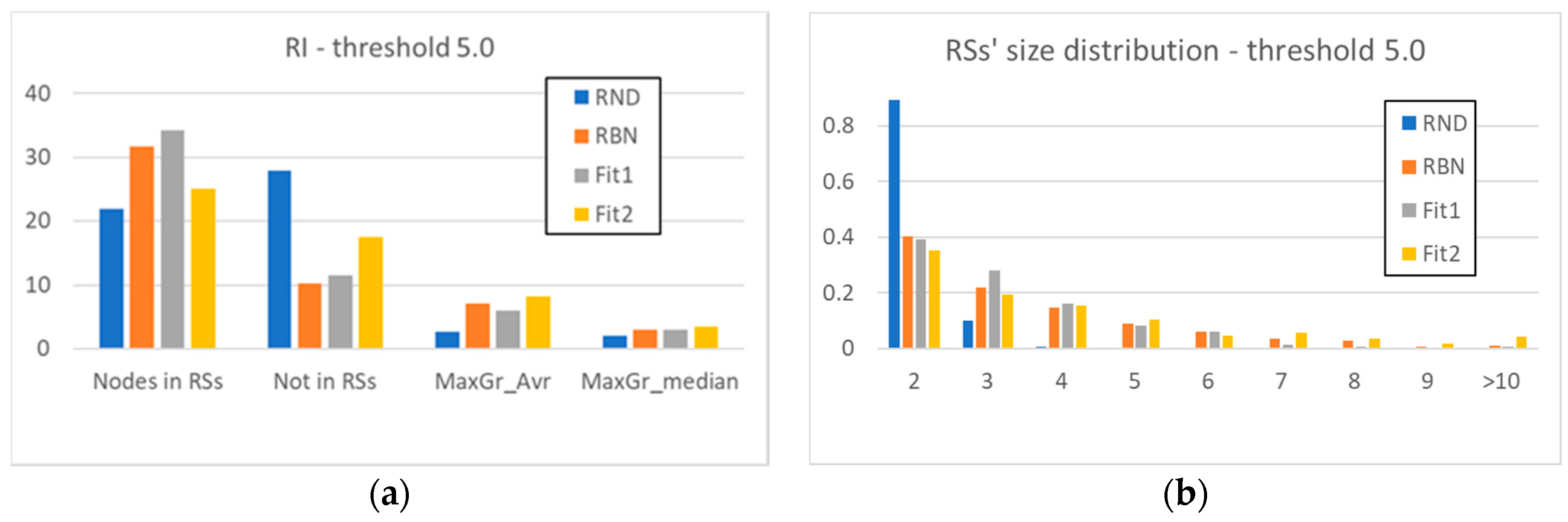
Figure 4a has a structure like that of Figure 2a: however, here we have also inserted the values of the Fit1 and Fit2 systems. We can note that the evolved systems maintain some characteristics of the RBN class: the nodes present within a RS are more than the nodes present within a RS in RND systems, as well as the mean and median size of the RSs. This situation confirms and better defines our earlier statement, that even the mere introduction of a topology—even if it is itself random—introduces a strong element of dynamic organization.
Another important remark is that the action of the GA can significantly change the static structure of the system (Fit1 case), or achieve the dynamic result without producing significant changes at the “architectural” level of the static components of the system (Fit2 case). The used indicators do not show large deviations: thus, it seems that evolution keeps track of the already present organization induced by the topology.
To observe the evolutionary changes, the indicators of Figure 4a are not sufficient, and it is necessary to examine in more detail the final distribution of the sizes of the RSs of the systems Fit1 and Fit2.
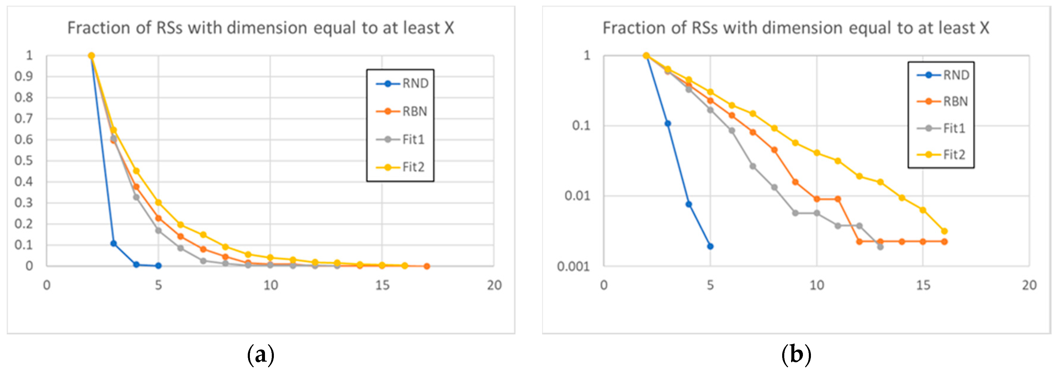
Figure 4b shows with the increase of the size of the groups a rapid disappearance of the RSs in the RND systems, and a persistence of the RSs of the other classes of systems. However, the distributions of the evolved systems seem to have different trends from those of the random systems: the size of the RSs of the Fit1 systems shows a small peak, and then decreases faster than the RND systems, while the Fit2 systems show a persistent presence of large groups.
These observations are confirmed by the data present in Figure 5, where the fraction of the groups that exceeds a certain size is shown: the distribution of the sizes of the RSs of the evolved systems deviates from the distribution of the RBN class. An interesting observation is that these deviations can have different directions: towards small groups (systems of the Fit1 class) or larger groups (systems belonging to Fit2 class).
4. Conclusions
The properties of many systems composed of many interacting elements are neither determined by the topology of the interaction network alone, nor by the dynamical laws in isolation, but they are the outcome of the interplay between topology and dynamics. (An interesting exception could be that of some systems exhibiting the so-called “swarm intelligence” [54,72], in which the topology of the interactions is variable and depends on the moves of the individual agents—in these cases, the topology can be seen as dependent on both the interaction rules and the history of the system. These systems are, however, outside the present discussion.) In this work we study this relationship by carrying out a systematic comparison on a particularly interesting and understood class of systems, a well-known model of gene regulatory dynamics.
We considered four different groups of structures with increasingly complex dynamical organization (loosely defined as the emergent property of the interactions between topology and dynamics, and identified by us through the distribution of the dynamic groups acting in the system), starting from a completely random situation to a situation with structure, up to organizations with structure and subject to evolution. All the involved systems are in (or very close to) critical dynamic regimes. Whenever possible, we have used analytic methods based on the static structure of the systems under investigation, while it has always been possible to use the dynamic analytic method.
A first significant observation is that the topology per se induces a notable increase in dynamic organization: to the best of our knowledge, this is the first case where this kind of dynamical organization in truly random BNs has actually been detected. It is also interesting that this organization cannot be deduced from observations of static nature, since the RND system has no static structure.
A second noteworthy observation is the fact that the dynamic organization of the classes of systems subjected to evolution does not consist of a large change in the distribution of the RSs: the evolutionary action supplied by the GA keeps track of the already present organization induced by the topology. A suggestive hypothesis on which it is worth working is that this situation may also be valid in other systems, or more in general for the same natural evolution.
Finally, and similarly to what happens in other applications of evolutionary algorithms to RBNs, the types of dynamic changes strongly depend upon the fitness function. Fit1 systems have fewer big RSs than random systems (the RBNs), while Fit2 systems, although involving fewer nodes in the RSs with respect to the other systems, have a greater number of big RSs. It should be noted that the static measurements are able to identify structural changes with respect to random systems (RBN) in Fit1 systems, while they are unable to detect anything significantly different from random systems in the case of Fit2 systems.
Alongside these three noteworthy observations, we could actually note that the fundamental contribution of this work is that of addressing the problem of quantitative identification of the dynamic organization of a system, and that of suggesting for this aim a method (the RI methodology) capable of identifying some interesting observables (the Relevant Sets). The identification of these structures allows a better observation and understanding of the phenomena under investigation, and often as consequence allows asking interesting new questions.
There are many interesting directions for future works: the two most stimulating seem to be the deepening of the possible mechanism of the re-use by evolution of the already existing dynamic organization, and the understanding of the dynamic interaction between the various RSs. Both directions require individual-level analysis.
In the first case, it is possible to keep track of the composition of the RSs in the parent-child sequence that leads from the initial random individual to the final one. In this case, it could be useful to use a learning algorithm without the horizontal exchange of information among individuals belonging to the same generation, as for example the stochastic descent, a strategy already used in RBN case [73], and verifying the distance distribution between these compositions: in the case of low distances, it can be concluded that evolution works based on the already existing dynamic organization, induced by the topology.
The second research line includes the characterization of the information exchange between the different RSs of the evolved individuals—for example by means of measures of information theory—with the consequent possibility of identifying their functional roles.
Author Contributions
Conceptualization, G.d., M.V., and R.S.; methodology, G.d., S.M., M.V., and R.S.; software, G.d., S.M., and M.V.; formal analysis, M.V.; writing, all authors (M.V. and R.S. coordinated much of the text; G.d. and S.M. have worked in a more dedicated way on Section 2 and Section 3). All authors have read and agreed to the published version of the manuscript.
Funding
This research was funded by FAR2019 project of the Department of Physics, Informatics and Mathematics of the University of Modena and Reggio Emilia.
Acknowledgments
We gratefully acknowledge the helpful discussions with Stuart Kauffman and Andrea Roli.
Conflicts of Interest
The authors declare no conflict of interest.
References
- Albert, R.; Barabási, A.L. Statistical mechanics of complex networks. Rev. Mod. Phys. 2002, 74, 47. [Google Scholar] [CrossRef] [Green Version]
- Albert, R.; Barabási, A.L. Emergence of Scaling in Random Networks. Science 1999, 286, 509–512. [Google Scholar] [CrossRef] [Green Version]
- Watts, D.; Strogatz, S. Collective dynamics of ‘small-world’ networks. Nature 1998, 393, 440–442. [Google Scholar] [CrossRef] [PubMed]
- Barrát, A.; Barthélemy, M.; Vespignani, A. Dynamical Processes on Complex Networks; Cambridge University Press: Cambridge, UK, 2008; ISBN 978-0-521-87950-7. [Google Scholar]
- Buldyrev, S.; Parshani, R.; Paul, G.; Stanley, H.E.; Havlin, S. Catastrophic cascade of failures in interdependent networks. Nature 2010, 464, 1025–1028. [Google Scholar] [CrossRef]
- Kitsak, M.; Gallos, L.K.; Havlin, S.; Liljeros, F.; Muchnik, L.; Stanley, H.E.; Makse, H.A. Identification of influential spreaders in complex networks. Nat. Phys. 2010, 6, 888–893. [Google Scholar] [CrossRef] [Green Version]
- Newman, M. Networks, 2nd ed.; Oxford University Press: Oxford, UK, 2018; ISBN 9780198805090. [Google Scholar]
- Pastor-Satorras, R.; Vespignani, A. Epidemic Spreading in Scale-Free Networks. Phys. Rev. Lett. 2001, 86, 3200. [Google Scholar] [CrossRef] [Green Version]
- Vespignani, A. The fragility of interdependency. Nature 2010, 464, 984–985. [Google Scholar] [CrossRef] [PubMed]
- Villani, M.; Filisetti, A.; Benedettini, S.; Roli, A.; Lane, D.; Serra, R. The detection of intermediate level emergent structures and patterns. In Proceeding of the ECAL 2013, the 12th European Conference on Artificial Life, Sicily, Italy, 2–6 September 2013; Liò, P., Miglino, O., Nicosia, G., Nolfi, S., Pavone, M., Eds.; MIT Press: Cambridge, MA, USA, 2013; pp. 372–378. ISBN 9780262317092. [Google Scholar]
- Villani, M.; Roli, A.; Filisetti, A.; Fiorucci, M.; Serra, R.; Poli, I. The Search for Candidate Relevant Subsets of Variables in Complex Systems. Artif. Life 2015, 21, 412–431. [Google Scholar] [CrossRef] [Green Version]
- Villani, M.; Sani, L.; Pecori, R.; Amoretti, M.; Roli, A.; Mordonini, M.; Serra, R.; Cagnoni, S. An Iterative Information-Theoretic Approach to the Detection of Structures in Complex Systems. Complexity 2018. [Google Scholar] [CrossRef]
- Sani, L.; Pecori, R.; Mordonini, M.; Cagnoni, S. From Complex System Analysis to Pattern Recognition: Experimental Assessment of an Unsupervised Feature Extraction Method Based on the Relevance Index Metrics. Computation 2019, 7, 39. [Google Scholar] [CrossRef] [Green Version]
- Villani, M.; Sani, L.; Amoretti, M.; Vicari, E.; Pecori, R.; Mordonini, M.; Cagnoni, S.; Serra, R. A Relevance Index Method to Infer Global Properties of Biological Networks. In Artificial Life and Evolutionary Computation. WIVACE 2017; Pelillo, M., Poli, I., Roli, A., Serra, R., Slanzi, D., Villani, M., Eds.; Springer: Berlin/Heidelberg, Germany, 2018; Volume 830, pp. 129–141. ISBN 978-3-030-21733-4. [Google Scholar]
- Sani, L.; Lombardo, G.; Pecori, R.; Fornacciari, P.; Mordonini, M.; Cagnoni, S. Social Relevance Index for Studying Communities in a Facebook Group of Patients. In Applications of Evolutionary Computation. EvoApplications 2018; Sim, K., Kaufmann, P., Eds.; Springer: Cham, Switzerland, 2018; Volume 10784, pp. 125–140. [Google Scholar] [CrossRef]
- Sani, L.; D’Addese, G.; Graudenzi, A.; Villani, M. The Detection of Dynamical Organization in Cancer Evolution Models. In Artificial Life and Evolutionary Computation. WIVACE 2019; Cicirelli, F., Guerrieri, A., Pizzuti, C., Socievole, A., Spezzano, G., Vinci, A., Eds.; Springer: Cham, Switzerland, 2020; Volume 1200, pp. 49–61. [Google Scholar] [CrossRef]
- Bastolla, U.; Parisi, G. The modular structure of Kauffman networks. Phys. D 1998, 115, 219–233. [Google Scholar] [CrossRef] [Green Version]
- Bastolla, U.; Parisi, G. Relevant elements, magnetization and dynamical properties in Kauffman networks: A numerical study. Phys. D 1998, 115, 203–218. [Google Scholar] [CrossRef] [Green Version]
- Drossel, B. Random Boolean networks. In Reviews of Nonlinear Dynamics and Complexity; Schuster, H.G., Ed.; Wiley-VCH: Weinheim, Germany, 2008; Chapter 1; pp. 69–110. ISBN 9783527407293. [Google Scholar]
- Aldana, M.; Coppersmith, S.; Kadanoff, L.P. Boolean dynamics with random couplings. In Perspectives and Problems in Nonlinear Science; Kaplan, E., Marsden, J., Sreenivasan, K.R., Eds.; Springer: New York, NY, USA, 2003; pp. 23–89. ISBN 9781468495669. [Google Scholar]
- Balleza, E.; Alvarez-Buylla, E.R.; Chaos, A.; Kauffman, S.A.; Shmulevich, I.; Aldana, M. Critical dynamics in genetic regulatory networks: Examples from four kingdoms. PLoS ONE 2008, 3, e2456. [Google Scholar] [CrossRef] [PubMed] [Green Version]
- Hidalgo, J.; Grilli, J.; Suweis, S.; Muñoz, M.A.; Banavarc, J.R.; Amos Maritan, A. Information-based fitness and the emergence of criticality in living systems. Proc. Natl. Acad. Sci. USA 2014, 111. [Google Scholar] [CrossRef] [Green Version]
- Kauffman, S.A. The Origins of Order; Oxford University Press: Oxford, UK, 1993; ISBN 9780195058116. [Google Scholar]
- Kauffman, S.A. At Home in the Universe; Oxford University Press: Oxford, UK, 1995; ISBN 0195111303. [Google Scholar]
- Langton, C.G. Computation at the edge of chaos: Phase transitions and emergent computation. Phys. D 1990, 42, 12–37. [Google Scholar] [CrossRef] [Green Version]
- Langton, C.G. Life at the edge of chaos. In Artificial Life II; Langton, C.G., Taylor, C., Farmer, J.D., Rasmussen, S., Eds.; Addison-Wesley: Redwood City, CA, USA, 1992; pp. 41–91. [Google Scholar]
- Muñoz, M.A. Criticality and dynamical scaling in living systems. Rev. Mod. Phys. 2018, 90, 031001. [Google Scholar] [CrossRef] [Green Version]
- Nykter, M.; Price, N.D.; Aldana, M.; Ramsey, S.A.; Kauffman, S.A.; Hood, L.E.; Yli-Harja, O.; Shmulevich, I. Gene expression dynamics in the macrophage exhibit criticality. Proc. Natl. Acad. Sci. USA 2008, 105, 1897–1900. [Google Scholar] [CrossRef] [Green Version]
- Packard, N.H. Adaptation toward the edge of chaos. In Dynamic Patterns in Complex Systems; World Scientific: Singapore, 1988; pp. 293–301. [Google Scholar] [CrossRef]
- Shmulevich, I.; Kauffman, S.A.; Aldana, M. Eukaryotic cells are dynamically ordered or critical but not chaotic. Proc. Natl. Acad. Sci. USA 2005, 102, 13439–13444. [Google Scholar] [CrossRef] [Green Version]
- Torres-Sosa, C.; Huang, S.; Aldana, M. Criticality is an emergent property of genetic networks that exhibit evolvability. PLoS Comput. Biol. 2012, 8, e1002669. [Google Scholar] [CrossRef] [Green Version]
- Beggs, J.M.; Timme, N. Being critical of criticality in the brain. Front. Physiol. 2012, 3, 163. [Google Scholar] [CrossRef] [Green Version]
- Roli, A.; Villani, M.; Filisetti, A.; Serra, R. Dynamical criticality: Overview and open questions. J. Syst. Sci. Complex 2018, 31, 647–663. [Google Scholar] [CrossRef] [Green Version]
- Villani, M.; Magrì, S.; Roli, A.; Serra, R. Evolving Always-Critical Networks. Life 2020, 10, 22. [Google Scholar] [CrossRef] [PubMed] [Green Version]
- Tononi, G.; Sporns, O.; Edelman, G.M. A measure for brain complexity: Relating functional segregation and integration in the nervous system. Proc. Natl. Acad. Sci. USA 1994, 91, 5033–5037. [Google Scholar] [CrossRef] [PubMed] [Green Version]
- Tononi, G.; McIntosh, A.; Russel, D.; Edelman, G. Functional clustering: Identifying strongly interactive brain regions in neuroimaging data. Neuroimage 1998, 7, 133–149. [Google Scholar] [CrossRef] [Green Version]
- Silvestri, G.; Sani, L.; Amoretti, M.; Pecori, R.; Vicari, E.; Mordonini, M.; Cagnoni, S. Searching Relevant Variable Subsets in Complex Systems Using K-Means PSO. In Artificial Life and Evolutionary Computation. WIVACE 2017; Pelillo, M., Poli, I., Roli, A., Serra, R., Slanzi, D., Villani, M., Eds.; Springer: Cham, Switzerland, 2018. [Google Scholar] [CrossRef]
- Sani, L.; Pecori, R.; Vicari, E.; Amoretti, M.; Mordonini, M.; Cagnoni, S. Can the Relevance Index be Used to Evolve Relevant Feature Sets? In Applications of Evolutionary Computation. EvoApplications 2018; Sim, K., Kaufmann, P., Eds.; Springer: Cham, Switzerland, 2018. [Google Scholar] [CrossRef]
- Kauffman, S.A. Metabolic stability and epigenesis in randomly constructed genetic nets. J. Theor. Biol. 1969, 22, 437–467. [Google Scholar] [CrossRef]
- Serra, R.; Villani, M.; Graudenzi, A.; Kauffman, S.A. Why a simple model of genetic regulatory networks describes the distribution of avalanches in gene expression data. J. Theor. Biol. 2007, 249, 449–460. [Google Scholar] [CrossRef] [PubMed]
- Wuensche, A. Genomic regulation modeled as a network with basins of attraction. Pac. Symp. Biocomput. 1998, 3, 89–102. [Google Scholar]
- Fernández, P.; Solé, R.V. The Role of Computation in Complex Regulatory Networks. In Power Laws, Scale-Free Networks and Genome Biology; Koonin, E.V., Wolf, Y.I., Karev, G.P., Eds.; Springer: Boston, MA, USA, 2006; pp. 206–225. ISBN 9780387339160. [Google Scholar] [CrossRef] [Green Version]
- Gershenson, C. Introduction to Random Boolean Networks. arXiv 2004, arXiv:nlin/0408006. [Google Scholar]
- Glass, L.; Kauffman, S.A. The logical analysis of continuous, non-linear biochemical control networks. J. Theor. Biol. 1973, 39, 103–129. [Google Scholar] [CrossRef]
- Shmulevich, I.; Dougherty, E.R.; Kim, S.; Zhang, W. Probabilistic Boolean networks: A rule-based uncertainty model for gene regulatory networks. Bioinformatics 2002, 18, 261–274. [Google Scholar] [CrossRef]
- Zañudo, J.G.T.; Aldana, M.; Martínez-Mekler, G. Boolean Threshold Networks: Virtues and Limitations for Biological Modeling. In Information Processing and Biological Systems; Niiranen, S., Ribeiro, A., Eds.; Springer: Berlin/Heidelberg, Germany, 2011. [Google Scholar] [CrossRef] [Green Version]
- Derrida, B.; Pomeau, Y. Random networks of automata: A simple annealed approximation. Europhys. Lett. 1986, 1, 45–49. [Google Scholar] [CrossRef]
- Derrida, B.; Flyvbjerg, H. The random map model: A disordered model with deterministic dynamics. J. Phys. 1987, 48, 971–978. [Google Scholar] [CrossRef]
- Holland, J.H. Adaptation in Natural and Artificial Systems; University of Michigan Press: Ann Arbor, MI, USA; MIT Press: Cambridge, MA, USA, 1975; ISBN 9780472084609. [Google Scholar]
- Sivanandam, S.N.; Deepa, S.N. Introduction to Genetic Algorithms; Springer: Berlin/Heidelberg, Germany, 2008; ISBN 978-3-540-73189-4. [Google Scholar]
- Bonabeau, E.; Dorigo, M.; Theraulaz, G. Swarm Intelligence: From Natural to Artificial Systems; Oxford University Press, Santa Fe Institute Studies in the Sciences of Complexity: New York, NY, USA, 1999; ISBN 0-19-513159-2. [Google Scholar]
- Darwish, A. Bio-inspired computing: Algorithms review, deep analysis, and the scope of applications. Future Comput. Inform. J. 2018, 3, 231–246. [Google Scholar] [CrossRef]
- Dorigo, M.; Maniezzo, V.; Colorni, A. Ant system: Optimization by a colony of cooperating agents. IEEE Trans. Syst. Man Cybern. Part B 1996, 26, 29–41. [Google Scholar] [CrossRef] [Green Version]
- Reynolds, C.W. Flocks, Herds, and Schools: A Distributed Behavioural Model Computer Graphics. In Proceedings of the 14th Annual Conference on Computer Graphics and Interactive Techniques, Anaheim, CA, USA, 27–31 July 1987; Volume 21, pp. 25–34. [Google Scholar] [CrossRef] [Green Version]
- Dulebenets, M.A.; Moses, R.; Ozguven, E.E.; Vanli, A. Minimizing carbon dioxide emissions due to container handling at marine container terminals via hybrid evolutionary algorithms. IEEE Access 2017, 5, 8131–8147. [Google Scholar] [CrossRef]
- Dulebenets, M.A.; Kavoosi, M.; Abioye, O.; Pasha, J. A self-adaptive evolutionary algorithm for the berth scheduling problem: Towards efficient parameter control. Algorithms 2018, 11, 100. [Google Scholar] [CrossRef] [Green Version]
- Anandakumar, H.; Umamaheswari, K. A bio-inspired swarm intelligence technique for social aware cognitive radio handovers. Comput. Electr. Eng. 2018, 71, 925–937. [Google Scholar] [CrossRef]
- Slowik, A.; Kwasnicka, H. Nature inspired methods and their industry applications—Swarm intelligence algorithms. IEEE Trans. Ind. Inform. 2018, 14, 1004–1015. [Google Scholar] [CrossRef]
- Zhao, X.; Wang, C.; Su, J.; Wang, J. Research and application based on the swarm intelligence algorithm and artificial intelligence for wind farm decision system. Renew. Energy 2019, 134, 681–697. [Google Scholar] [CrossRef]
- Yang, X.S. Flower Pollination Algorithm for Global Optimization. In Unconventional Computation and Natural Computation. UCNC 2012; Durand-Lose, J., Jonoska, N., Eds.; Springer: Berlin/Heidelberg, Germany, 2012. [Google Scholar] [CrossRef] [Green Version]
- Uymaz, S.A.; Tezel, G.; Yel, E. Artificial algae algorithm (AAA) for nonlinear global optimization. Appl. Soft Comput. 2015, 31, 153–171. [Google Scholar] [CrossRef]
- Yang, X.S. A New Metaheuristic Bat-Inspired Algorithm. In Nature Inspired Cooperative Strategies for Optimization (NICSO 2010). Studies in Computational Intelligence; González, J.R., Pelta, D.A., Cruz, C., Terrazas, G., Krasnogor, N., Eds.; Springer: Berlin/Heidelberg, Germany, 2010. [Google Scholar] [CrossRef] [Green Version]
- Pradhan, P.M.; Panda, G. Solving multiobjective problems using cat swarm optimization. Expert Syst. Appl. 2012, 39, 2956–2964. [Google Scholar] [CrossRef]
- Mirjalili, S.; Lewis, A. The whale optimization algorithm. Adv. Eng. Soft. 2016, 95, 51–67. [Google Scholar] [CrossRef]
- Deb, S.; Fong, S.; Tian, Z. Elephant search algorithm for optimization problems. In Proceedings of the Tenth International Conference on Digital Information Management (ICDIM 2015), Jeju Island, Korea, 21–23 October 2015; pp. 249–255. [Google Scholar] [CrossRef]
- Mirjalili, S.; Mirjalili, S.M.; Lewis, A. Grey wolf optimizer. Adv. Eng. Softw. 2014, 69, 46–61. [Google Scholar] [CrossRef] [Green Version]
- Meng, X.; Liu, Y.; Gao, X.; Zhang, H. A New Bioinspired Algorithm: Chicken Swarm Optimization; Springer: Cham, Switzerland, 2014; Part I; pp. 86–94. [Google Scholar] [CrossRef]
- Yang, X.-S.; Deb, S. Cuckoo search via Lévy flights. In Proceedings of the World Congress on Nature & Biologically Inspired Computing (NaBIC 2009), Coimbatore, India, 9–11 December 2009; pp. 210–214, ISBN 978-1-4244-5053-4. [Google Scholar]
- Elbeltagi, E.; Hegazy, T.; Dnald, G.D. Comparison among five evolutionary-based optimization algorithms. Adv. Eng. Inform. 2005, 19, 43–53. [Google Scholar] [CrossRef]
- Hughes, T.R.; Marton, M.J.; Jones, A.R.; Roberts, C.J.; Stoughton, R.; Armour, C.D.; A Bennett, H.; Coffey, E.; Dai, H.; He, Y.D.; et al. Functional discovery via a compendium of expression profiles. Cell 2000, 102, 109–126. [Google Scholar] [CrossRef] [Green Version]
- Corder, G.W.; Foreman, D.I. Nonparametric Statistics: A Step-by-Step Approach; Wiley: New York, NY, USA, 2014; ISBN 978-1118840313. [Google Scholar]
- Beni, G.; Wang, J. Swarm Intelligence in Cellular Robotic Systems. In Robots and Biological Systems: Towards a New Bionics? NATO ASI Series (Series F: Computer and Systems Sciences); Dario, P., Sandini, G., Aebischer, P., Eds.; Springer: Berlin/Heidelberg, Germany, 1993. [Google Scholar] [CrossRef]
- Roli, A.; Manfroni, M.; Pinciroli, C.; Birattari, M. On the Design of Boolean Network Robots. In Applications of Evolutionary Computation. EvoApplications 2011; Di Chio, C., Ed.; Springer: Berlin/Heidelberg, Germany, 2011. [Google Scholar] [CrossRef] [Green Version]
Figure 1.
The average number of performed avalanches (red) and the average number of nodes involved in at least one avalanche (green), for the four classes of system under examination (50 systems composed by 50 nodes in each classes).
Figure 1.
The average number of performed avalanches (red) and the average number of nodes involved in at least one avalanche (green), for the four classes of system under examination (50 systems composed by 50 nodes in each classes).

Figure 2.
The average number of nodes present within the RSs identified in random avalanches and in avalanches occurring in critical RBN, the average number of nodes excluded from them, and the average (MaxGr_Avr) and median (MaxGr_Median) size of the maximum size RS. (a) RI analysis with threshold θ5; (b) RI analysis with threshold θ3.

Figure 3.
The observed frequency of the Boolean function present in evolved systems vs. the frequency characteristic of RBN class (uniform distribution, red line). The vertical dotted line separates on the left the Boolean functions which to an input of double “1” correspond to an output equal to “0”, and on the right the Boolean functions that correspond an output equal to “1”. The red ellipses highlight the cases of significant deviations from the hypothesis of uniform distribution (at the level of 1%). (a) Fit1 class systems; (b) Fit2 class systems.

Figure 4.
(a) The average number of nodes present within the RSs identified in the systems under examination, the average number of nodes excluded from them, and the average (MaxGr_Avr) and median (MaxGr_Median) size of the maximum size RS (RI threshold θ5). (b) The detailed RSs’ size distribution (RI threshold θ5).

Figure 5.
The fraction of RSs, on the total of all RSs identified in the 50 systems (for each type) under examination, with size equal to at least the value on the X axis, linear (a) and logarithmic (b) scale. The dynamic organization of RBNs involves a number of large RSs that is much higher than that of large RSs randomly present in random avalanches. The action of evolution modified this dynamic organization in different directions for different fitness (amplifying or reducing the dimensions of the RSs).


Table 1.
The parameter values used during simulations. In order to characterize the systems under analysis, when necessary (searching for attractors, determination of the Derrida parameter), we used 10,000 initial conditions. The used BNs are composed by nodes having two inputs each: RBNs with this topology have a critical regime if their bias is equal to 0.5.
| System | Parameter | Value |
|---|---|---|
| GA | number of generations | 100 |
| GA | number of RBNs in population | 100 |
| GA | crossover probability | 0.7 |
| GA | mutation probability per node | 0.02 |
| GA | number of best individuals directly transmitted to next generation (elitism) | 3 |
| BN | number of nodes per BN | 50 |
| BN | number of inputs per node | 2 |
| BN | average initial bias in initial population | 0.5 |
| BN | number of initial conditions per BN | 10,000 |
Publisher’s Note: MDPI stays neutral with regard to jurisdictional claims in published maps and institutional affiliations. |
© 2020 by the authors. Licensee MDPI, Basel, Switzerland. This article is an open access article distributed under the terms and conditions of the Creative Commons Attribution (CC BY) license (http://creativecommons.org/licenses/by/4.0/).
Share and Cite
MDPI and ACS Style
d’Addese, G.; Magrì, S.; Serra, R.; Villani, M. Exploring the Dynamic Organization of Random and Evolved Boolean Networks. Algorithms 2020, 13, 272. https://0-doi-org.brum.beds.ac.uk/10.3390/a13110272
AMA Style
d’Addese G, Magrì S, Serra R, Villani M. Exploring the Dynamic Organization of Random and Evolved Boolean Networks. Algorithms. 2020; 13(11):272. https://0-doi-org.brum.beds.ac.uk/10.3390/a13110272
Chicago/Turabian Styled’Addese, Gianluca, Salvatore Magrì, Roberto Serra, and Marco Villani. 2020. "Exploring the Dynamic Organization of Random and Evolved Boolean Networks" Algorithms 13, no. 11: 272. https://0-doi-org.brum.beds.ac.uk/10.3390/a13110272
Note that from the first issue of 2016, this journal uses article numbers instead of page numbers. See further details here.