Combining Optimization and Simulation for Designing a Robust Short-Sea Feeder Network
by
 , and
, and
Carl Axel Benjamin Medbøen
, 
Magnus Bolstad Holm
,
Mohamed Kais Msakni
*,
Kjetil Fagerholt
and
Peter Schütz
Department of Industrial Economics and Technology Management, Norwegian University of Science and Technology, 7491 Trondheim, Norway
*
Author to whom correspondence should be addressed.
Algorithms 2020, 13(11), 304; https://0-doi-org.brum.beds.ac.uk/10.3390/a13110304
Submission received: 5 October 2020
/
Revised: 11 November 2020
/
Accepted: 16 November 2020
/
Published: 20 November 2020
(This article belongs to the Special Issue Simulation-Optimization in Logistics, Transportation, and SCM)
Abstract
:Here we study a short-sea feeder network design problem based on mother and daughter vessels. The main feature of the studied system is performing transshipment of cargo between mother and daughter vessels at appropriate locations at sea. This operation requires synchronization between both types of vessels as they have to meet at the same location at the same time. This paper studies the problem of designing a synchronized feeder network, explicitly accounting for the effect of uncertain travel times caused by harsh weather conditions. We propose an optimization-simulation framework to find robust solutions for the transportation system. The optimization model finds optimal routes that are then evaluated by a discrete-even simulation model to measure their robustness under uncertain weather conditions. This process of optimization simulation is repeated until a satisfactory condition is reached. To find even better solutions, we include different performance-improving strategies by adding robustness during route generation or exploiting flexibility in sailing speed to recover from delays. We apply the solution method to a case based on realistic data from a Norwegian shipping company. The results show that the method finds near-optimal solutions that offer robustness against schedule perturbations due to harsh weather. They also highlight the importance of considering uncertainty when designing a short-sea feeder network with transshipment at sea.
1. Introduction
Maritime transportation is one of the most efficient (per cargo ton-mile) transportation modes to transport large volumes of cargo over long distances [1,2]. Over short distances, however, competing with road-based transportation is more challenging. Truck-based door-to-door deliveries are often less expensive compared to other shipping solutions and offer frequent and reliable departures [3,4].
The demand for cargo transportation in Norway is expected to grow by 40% (in tonne-kilometers) until 2030 [5]. This predicted increase i is met by the political ambition to shift more goods from road to sea [6]. Still, new and innovative solutions need to be developed to substantially improve the competitiveness of short-sea shipping and support the transition of cargo from road-based to waterborne transportation. The Short Sea Pioneer (SSP) logistics system is a new suggested solution to improve competitiveness, proposing a new transshipment mode for short-sea feeder networks [7]. The proposed system is inspired by the ship-to-ship cargo transfer method currently used to transfer petroleum products and bulk cargo between seagoing vessels. In the SSP system, a mother (large) vessel can be connected to a daughter (small feeder) vessel at a suitable location at sea to transship containerized cargo using a specialized handling cargo system (see [8] for an illustration). One advantage of this system is to reduce the number of port calls, which reduces the operational cost of the shipping system. Indeed, cargo-related port costs can account for up to 30% of the turnover of a smaller short-sea shipping company [9]. Besides, it becomes possible to serve small ports that large vessels cannot visit, for example, due to physical limitations.
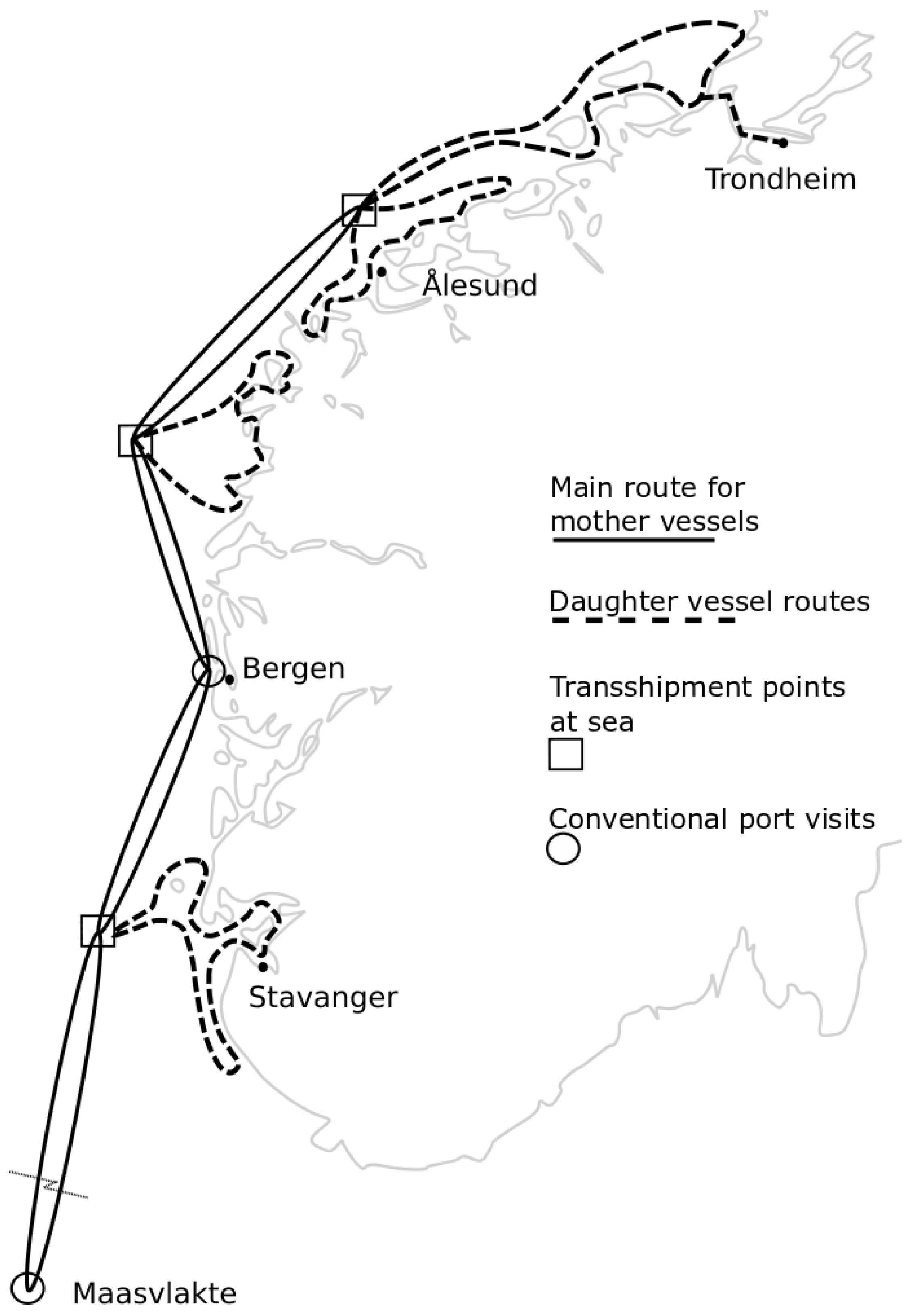
The SSP logistics system is composed of one main route sailed by mother vessels that transport cargo between the European continent and large ports located at the Norwegian west coast. Small daughter vessels operate feeder routes serving smaller Norwegian ports. Due to size or location, these ports may only be served by the smaller daughter vessels. Potential candidate transshipment locations will be in sheltered locations (e.g., inside a fjord or inshore) such that harsh weather does not affect the transshipment operation. An example is illustrated in Figure 1.
While potentially having considerable economic benefits, transshipment at sea also raises many technical challenges. Among others, the system requires synchronizing the main route sailed by the mother vessel with all routes sailed by the daughter vessels. Conversely, Weather conditions are known to impact sailing times and can cause considerable delays [2]. Thus, the synchronization operation can be subject to disruptions that may cause additional waiting times at the transshipment location and can propagate through the system for the subsequent periods. To function correctly, the routes for both mother and daughter vessels need to be robust to potential delays, i.e., they have to account for uncertainty in weather conditions.
Traditionally, the literature on liner shipping network design problems has been focusing on deterministic deep-sea (long-haul) shipping networks. These problems usually determine the optimal set of routes to be served by a heterogeneous fleet of vessels while satisfying demand, transshipment, and frequency requirements (see, e.g., Brouer et al. [11] ). The following publications are recent examples, discussing different variants of the traditional liner network design problem. Meng and Wang [12] include the repositioning of empty containers in the shipping operations when determining the optimal network design. Reinhardt and Pisinger [13] consider more advanced route structures, such as butterfly routes, because they allow for better use of vessel resources. Brouer et al. [11] study one of the largest networks operated by a major liner-shipping company, where cargo can be transshipped several times to take more than one route to be delivered. Karsten et al. [14] extend this problem to include transit time restrictions. Balakrishnan and Karsten [15] incorporate limitations on number of transshipments for the cargo. For the short-sea shipping, Msakni et al. [16] study the impact of different network designs for a local liner shipping company. Fadda et al. [17] address the problem of a roll-on roll-off liner service that operates using a hub-and-spoke network design. Akbar et al. [18] provide an economic analysis of introducing autonomous vessels in short-sea shipping. For a more detailed overview of the literature on liner shipping network design, please also see the surveys by Meng et al. [19], Brouer et al. [1] and Christiansen et al. [20].
Synchronization has received relatively little attention in the literature on maritime transportation. Cargo is usually transshipped in ports, often requiring a sequence of arrivals or specifying a time window. The work of Agarwal and Özlem Ergun [21] is one of the fewest papers to address synchronization directly. The problem considers a combined vessel scheduling and cargo routing problem, where transshipment of cargo is only possible when two routes meet at the same port on the same day. In another work, Andersson et al. [22] study a problem from project shipping where different cargoes may require a synchronized delivery. In land-based transportation, synchronization issues are more common. The reader is referred to Drexl [23] for an overview of the literature on VRPs with multiple synchronization constraints.
The research on uncertainty in maritime service networks mainly distinguishes between two types of uncertainty. The first type is uncertainty in service times, usually port times or sailing times, whereas the second type considers uncertainty in demand. When considering uncertainty in operations, the research focuses on keeping a designed schedule, i.e., satisfy frequency requirements or pickup and delivery time windows. As an example of this work line, the problem examined by Wang and Meng [24] of designing liner vessel routes with uncertainty in port operation times. The uncertainty is related to sailing times as a consequence of making up for the delays. In Song et al. [25], a multi-objective liner shipping service problem with uncertain port times is studied. One of the objectives is to minimize schedule unreliability, which is the probability of the vessels arriving after the scheduled time windows. Conversely, Li et al. [26] study how vessels can recover from delays caused by regular uncertainties and unexpected disruptions. In their work, regular uncertainties may happen both at sea and in port, and their characteristics can be estimated using historical data. When it comes to demand uncertainty, the research usually focuses on designing a maritime transportation system such that demand can be served. For example, Ng and Lin [27] study the problem of fleet deployment under incomplete demand information. Lo et al. [28] present a model for designing a ferry network given uncertain demand. An and Lo [29] study the design of more general transit networks under uncertain demand. However, none of these studies consider uncertainty in service times.
One approach to deal with the uncertainty is to combine simulation and optimization models to provide robust solutions. Fischer et al. [30] use simulation and optimization to evaluate the robustness of tactical fleet deployment plans for roll-on roll-off liner shipping with respect to random disruptions at the operational level. Castilla-Rodríguez et al. [31] study the quay crane scheduling problem in a port terminal and consider the uncertainty from the availability of some delivery vehicles and disruptions in quay crane operations. The authors use simulation-optimization to produce robust quay crane schedules. Layeb et al. [32] develop a simulation-optimization method for multimodal freight transportation systems where the uncertainty is related to demand and travel times. Poeting et al. [33] combine a metaheuristic with a discrete-event simulation to provide robust solutions at the operational level in parcel transshipment terminals.
This paper considers the first type of uncertainty, more specifically uncertain sailing times due to harsh weather conditions. However, in contrast to the papers mentioned above, it studies a short-sea liner network instead of a deep-sea network. A common assumption in papers on deep-sea liner network design with uncertain port times is that vessels can make up for delays by increasing their speed between ports (see, e.g., Wang and Meng [24]). This can be reasonable when legs between ports are long. However, for short-sea networks, the sailing legs are short, and weather conditions may prevent the vessel from reducing or even eliminating a delay.
The problem presented in this paper is an extension to the deterministic Short-sea Liner Network Design Problem with Transshipment at Sea (SLNDP-TS) introduced by Holm et al. [10]. It contributes to the research literature on liner shipping network design in three ways. Firstly, we take into account uncertain sailing times due to harsh weather in the network design problem. Secondly, we consider transshipments at sea, which requires that the synchronization of routes to ensure that mother and daughter vessels are at the same location at the same time. Thirdly, we apply an iterative solution approach combining optimization with discrete event simulation to handle both uncertainties in sailing times and synchronization requirements.
Our solution method is based on the hybrid optimization-simulation method proposed by Acar et al. [34] with the difference of using a discrete-event model instead of an optimization model for the simulations. Unlike commonly used probabilistic models, we use wave height from historical weather data to adequately capture the effect of harsh weather conditions on sailing speed. The simulation model links wave height to vessel speed and evaluates the impact on the synchronization operations. The simulation results are returned to the optimization model to select routes that are less likely to generate delays. Additionally, we develop and test different performance-improving strategies to enhance the solutions’ robustness to possible delays. The computational study results show that our approach provides more robust solutions than deterministic ones without a significant increase in costs.
The remainder of this paper is structured as follows. In Section 2, the problem is described in more detail. Section 3 outlines the solution approach. The optimization and simulation models are presented in more detail in Section 4. Results from the computational study are presented in Section 5. We conclude in Section 6.
2. Problem Description
The problem of designing a short-sea liner network with transshipment at sea has been introduced by Holm et al. [10]. The authors provide a deterministic problem formulation as well as a solution method based on a priori route generation. In this section, we first present the problem before discussing the impact of weather conditions on shipping operations in such a network.
2.1. Network Design Problem
The shipping company serves each port on a weekly basis. The Norwegian ports are classified according to their size. Small ports are only served by daughter vessels, whereas large ports can be visited by either a mother or a daughter vessel. All mother vessels start their voyage at a European continental main port. Transshipment of cargo between mother and daughter vessels occurs at the so-called ocean hubs, which are suitable locations along the Norwegian coast and offer enough stability for vessels to perform transshipment at sea. For presentation and modeling purposes, each ocean hub is artificially split into a north-going and a south-going ocean hub. A mother vessel serves a north-going ocean hub during its northbound journey and a south-going ocean hub on its southbound journey.
The feeder routes taken by daughter vessels are referred to as daughter routes. Each daughter route is served by one daughter vessel. These routes have a maximum duration of one week to ensure weekly port visits. The route served by the mother vessel is referred to as main route. Since the duration of the main route is typically more than one week, the number of deployed mother vessels is equal to the number of weeks rounded up to the nearest integer, thus ensuring weekly service.
The major activity of the shipping company case is to transport cargo between the main continental port and Norwegian ports. There is also some local demand between Norwegian ports, but can be considered as negligible in this study. The aim is to determine the optimal main and daughter routes and the optimal fleet of mother and daughter vessels to be deployed. This problem is at a tactical level, where the established routes last for typically four to 12 months, and, therefore, the weekly demand is assumed to be known and constant.
Transshipment of cargo between mother and daughter vessels is only possible at ocean hubs. During its northbound journey, mother and daughter vessels meet at a north-going ocean hub where cargo is delivered to the daughter vessel. The same mother and daughter vessels meet again at the corresponding south-going ocean hub during the southbound journey of the mother vessel to transship cargo from the daughter vessel. In the case an ocean hub is the northernmost point of the main route, there is no artificial distinction between north- and south-going ocean hub, and the ocean hub is therefore only visited once.
A solution to the problem consists of a set of main and daughter routes serving the ports and an allocation of vessels to routes (as illustrated in Figure 1). This also includes determining the number of deployed mother and daughter vessels. The mother vessels are considered to have enough capacity to transport all cargo. The size of the daughter vessels can be selected from a given set of available capacities. The problem is separable in the size of the daughter vessel because all daughter vessels must have the same capacity due to the technical requirements of the SSP design. The objective is to minimize the weekly operating costs, including weekly time charter costs for each vessel in the selected fleet, bunker, port, and cargo handling costs.
2.2. Impact of Harsh Weather
A transshipment in an ocean hub requires that both the mother vessel and the daughter vessel have to be present at the same location at the same time. The meeting point is selected in a sheltered location, such that harsh weather will not affect the transshipment operation. However, harsh weather conditions will affect sailing operations as they may force vessels to slow down, causing delays in the vessels’ schedules. We refer to the situation of a mother vessel waiting for a daughter vessel in an ocean hub as a synchronization violation. Synchronization violations delay the waiting vessel, potentially delaying later synchronizations and affecting other vessels in the system.
If a vessel is delayed by too much, it might be unable to complete its route within the maximum allowed duration. This is called a duration violation. Duration violations prevent a weekly port visit frequency because the delay is transferred into the next week. For a logistics system with transshipment at sea to be viable in practice, duration violations must be kept at a minimum.
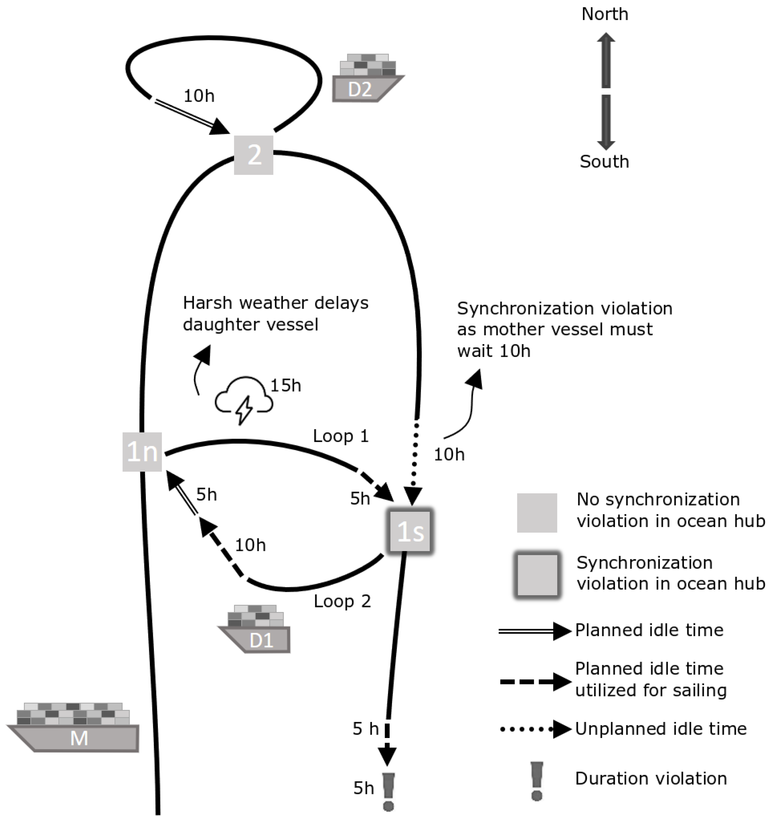
Figure 2 illustrates synchronization and duration violations. Consider a logistics system consisting of a mother vessel, M, and two daughter vessels, D1 and D2. Daughter vessel D1 visits the north- and south-going ocean hubs, 1n and 1s, respectively. The mother vessel and Daughter vessel D2 meet at ocean hub 2 for picking-up and delivering cargo because ocean hub 2 is the northernmost point. For simplicity, Norwegian ports and the continental main ports are not shown.
In the example, the mother vessel is sailing north from the continental main port. In ocean hub 1n, she meets with daughter vessel D1, and after the transshipment, both vessels depart as scheduled. Neither of the vessels is delayed at this point. The mother vessel continues north to ocean hub 2 without any delay. Daughter vessel D2 is not delayed either, and thus both vessels can synchronize as planned in ocean hub 2. In this example, daughter vessel D2 has 10 h of planned idle time before the arrival of the mother vessel. It could, therefore, be up to 10 h delayed and still synchronize with the arriving mother vessel as scheduled.
After leaving ocean hub 2, the mother vessel starts its southbound journey and sails towards ocean hub 1s to synchronize again with daughter vessel D1. However, harsh weather has caused a delay for daughter vessel D1 after departing from ocean hub 1n. Despite arriving on time in ocean hub 1s, the mother vessel has to wait for daughter vessel D1 and experiences a synchronization violation.
The schedule for daughter vessel D1 has planned idle time of five hours in ocean hub 1s before the arrival of the mother vessel. As the vessel is delayed by as much as 15 h, the mother vessel has to wait for 10 h. As the mother vessel only has five hours of planned idle time in its schedule, the next departure from the continental main port is five hours of delay. The synchronization violation in ocean hub 1s has caused a duration violation of five hours for the mother vessel.
Note that daughter vessel D1 does not incur a duration violation, even though it is 10 h delayed when leaving ocean hub 1s. This is because there is enough planned idle time when sailing between ocean hub to 1s and ocean hub 1n to make up for the delay.
3. Solution Approach
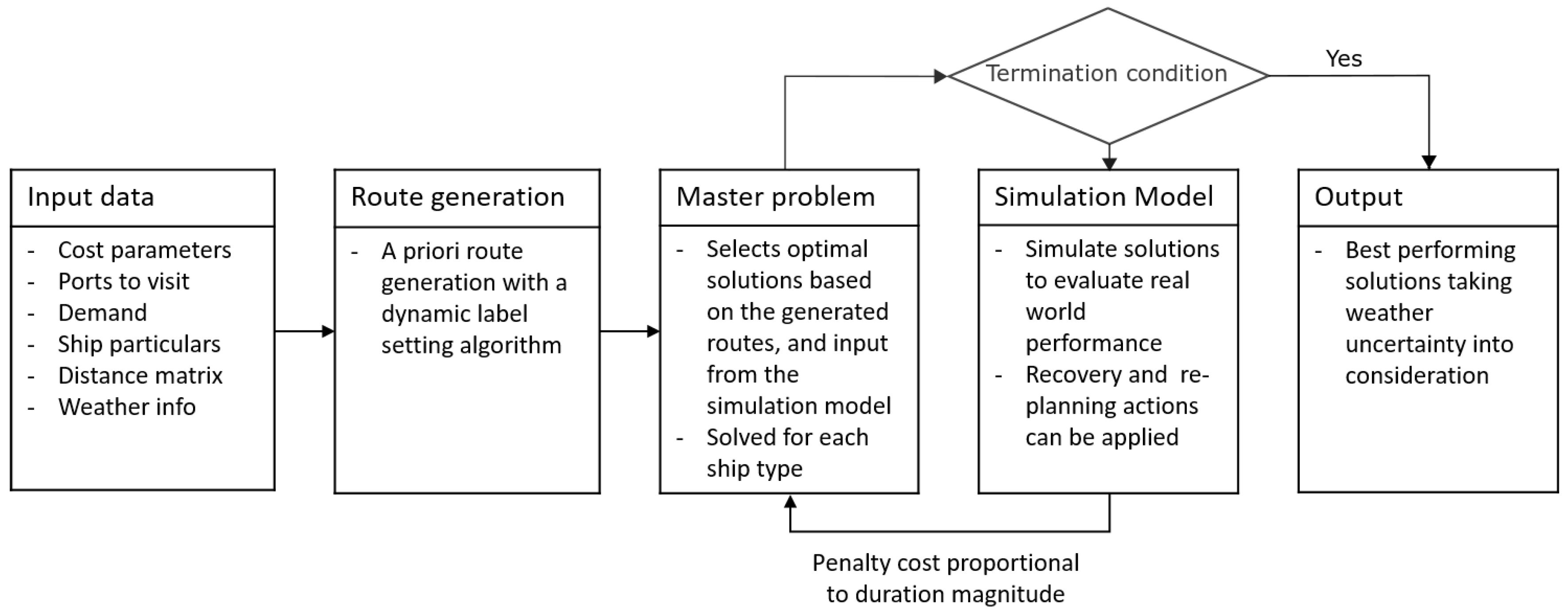
Our iterative solution method is based on the hybrid optimization simulation framework proposed by Acar et al. [34]. The solution method combines an optimization model (also referred to as the master problem) and a simulation model. The role of the optimization model is to select routes for mother and daughter vessels from a set of a priori generated routes, while the simulation is a discrete event simulation model that evaluates the robustness of solutions (a solution is a combination of routes) with respect to uncertain weather conditions. The simulation model results are used to update the costs of the simulated solutions and then faded back to the optimization model. Alternating between optimization and simulation models is repeated until no new improved solution is found. The proposed solution method is illustrated in Figure 3. According to the classification of Crainic et al. [35], the proposed approach is within the alternate simulation-optimization category.
A static set of routes for the mother and daughter vessels is generated using the provided input data. For each of the daughter vessel types, the master problem then selects the cost-minimizing routes from this set by solving an integer programming model (described in more detail in Section 4.1). Afterwards, the combination of routes chosen by the master problem is simulated using historical weather data to estimate the solution’s real-world performance (described in more detail in Section 4.2).
As explained in Section 2.2, a duration violation is caused by harsh weather conditions that lead to a delay long enough to prevent the vessel from completing its round trip within its scheduled duration. Synchronization violations can amplify delays as they may transfer the delay of one vessel to another. A duration violation will automatically lead to an initial disruption when starting the next round trip. The magnitude of a duration violation is defined as the number of hours by which a vessel is late compared to the allowed duration of one round trip.
We add a penalty cost based on the magnitude of duration violations from the simulation to the costs of the selected combination of routes. This additional penalty cost makes solutions (or route combinations) prone to duration violations less attractive in subsequent iterations of solving the master problem. When the master problem is solved again with updated route costs, it might choose a new solution with lower costs. The iterations between the master problem and the simulation model continue until all of the selected solutions have been simulated, and no new improving solutions are found. This feedback approach between the master problem and the simulation model allows generating good solutions based on the trade-off between operational costs and robustness (i.e., penalty costs).
Different strategies to provide robustness against disruptions due to harsh weather and/or synchronization violations can be included in the optimization and/or simulation model (discussed more in Section 4.3). Thus, the framework can also be used to evaluate the potential benefit of introducing performance-improving strategies, for example, permitting speed-ups in case of a delay (see, e.g., Fischer et al. [30], Brouer et al. [36]).
4. Optimization and Simulation Model
This section provides a more detailed description of the optimization and the simulation models used in the proposed solution method. The optimization model is described in Section 4.1, while the simulation model is presented in Section 4.2. Possible performance-improving strategies that can be evaluated using our solution methods are described in Section 4.3.
4.1. Optimization Model
The optimization model is based on the approach developed by Holm et al. [10] and consists of a route generation procedure and a master problem. The difference is that, in this study, the optimization model incorporates updated costs from the simulation model. For an efficient route generation, a label-setting algorithm (see, e.g., Irnich [37]) is used to generate a priori the routes for mother and daughter vessels. After the routes are generated, the daughter routes are grouped in subsets according to which main route they can be synchronized with.
The label setting algorithm is used to limit the set of routes introduced to the optimization model. Only non-dominated routes are retained, which means that similar routes composed of the same ports but in a different order and with higher operational costs are eliminated. The route generation assumes that vessels sail at their design sailing speed, i.e., no speed-up is allowed. Here, it should be pointed out that some of the deterministically dominated routes might perform better in our setting with uncertain travel time, e.g., due to a sequence of port visits that allows avoiding harsh weather conditions. However, identifying these routes during the route generation procedure is, in general, too computationally expensive.
Before formulating the optimization model, let us first introduce the following notation:
Sets
- set of ocean hubs,
- set of Norwegian small ports,
- set of Norwegian main ports,
- set of all non-dominated main routes,
- set of all non-dominated daughter routes,
- subset of main routes, for which port p is served, ,
- subset of daughter routes, for which port p is served, ,
- subset of daughter routes that can be synchronized to a main route m at ocean hub p, ,
- set of simulated solutions. If the set is empty, no solutions have been simulated. The size of the set increases for every new solution that is simulated.
Parameters
- total operational cost of main route m, which includes the weekly time charter cost of mother vessels sailing m, bunker costs and port costs,
- operational cost of daughter route d, which includes the weekly time charter cost of daughter vessel sailing d, bunker costs and port costs,
- penalty cost of simulated solution s,
- upper limit on the number of daughter vessels that can perform transshipment at an ocean hub,
- a value that is marginally larger than ,
- is equal to 1 if daughter route d belongs to simulated solution s, and 0 otherwise,
- is equal to 1 if main route m belongs to simulated solution s, and 0 otherwise,
- number of routes which belong to solution s. This can be expressed as follows: , for each simulated solution s,
- auxiliary parameter used to express a less than relation as a less than or equal relation. The value can be as small as possible as long as .
Binary decision variables
- equals to 1 if main route m is selected, and 0 otherwise,
- equals to 1 if daughter route d is selected, and 0 otherwise,
- takes value 1 if a simulated solution is included in the optimal solution, and 0 otherwise.
The deterministic optimization problem can be formulated as follows:
subject to
The objective function (1) minimizes the total weekly cost of the shipping system. The first and second terms of (1) are related to the costs of mother and daughter vessels deployed in the system. The last term represents the penalty cost of a solution.
Equation (2) forces the optimal solution to select only one main route. Constraints (3) to (5) are the synchronization constraints, ensuring that selected daughter routes can synchronize with the main route at an ocean hub visited by both routes. The reader is referred to Holm et al. [10] for a more detailed description of how synchronization is taken care of through these constraints. Further, Equation (6) ensure that a main port is visited by either a mother or a daughter vessel. Equations (7) ensure that each small Norwegian port is served by a daughter route. Constraints (8) set the indicator variable . If the master problem selects a route combination that constitutes a previously simulated solution, and the penalty cost is added to the objective. Lastly, Constraints (9)–(11) restrict the variables to take binary values.
4.2. Simulation Model
The optimal solution of the master problem assumes that the shipping system runs under perfect weather conditions, and both mother and daughter vessels sail at design speed. The simulation model evaluates the proposed solution under real-world operating conditions. Harsh weather conditions may force vessels to slow down, affecting the sailing times. In such a situation, synchronization and duration violations can occur.
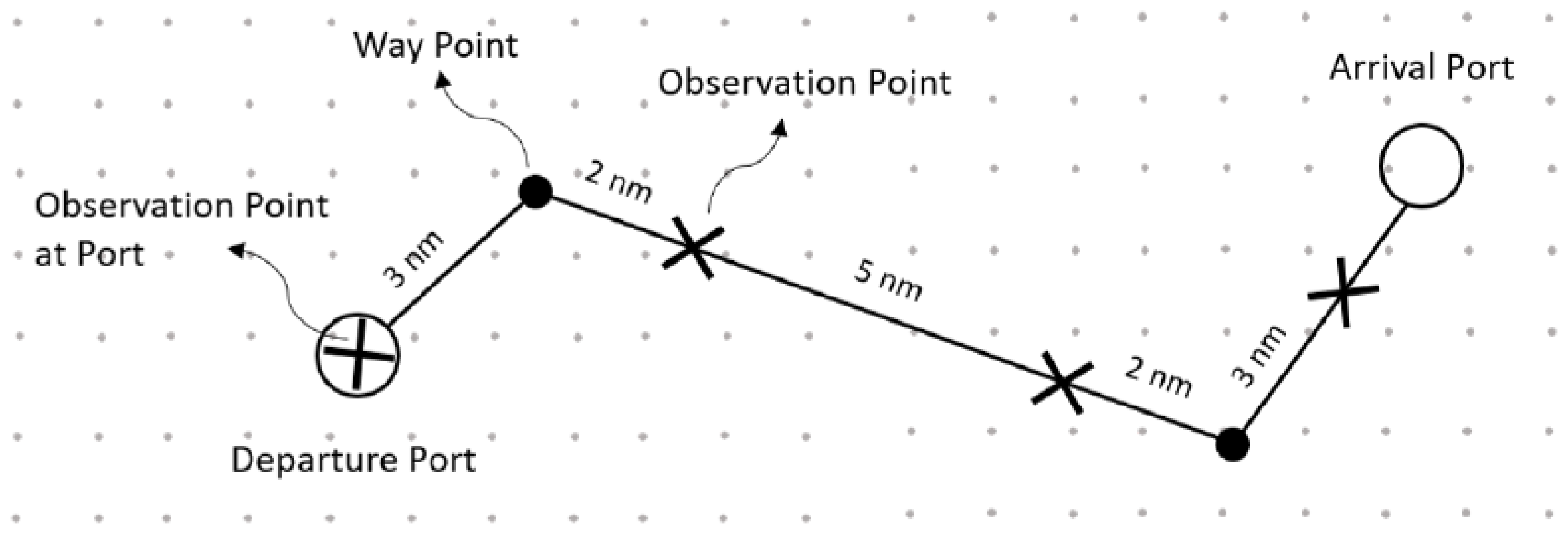
The simulation model adjusts the sailing speed based on wave height. To this end, we divide a route into legs connecting two consecutive ports. For a given leg, waypoints are defined and mark a change in the vessel’s travel direction. The segment between two successive waypoints is defined as a sub-leg. The simulation model updates the sailing speed of a vessel at specific points of a leg. Such a point is called an observation point and is defined (i) at a departure port and (ii) after sailing a certain distance, called step distance.
Figure 4 shows an example of a route between two ports. There are three sub-legs defined by the ports and waypoints. The observation points are equally separated by the step distance, which is set to be five nautical miles in this example. The background of Figure 4 shows the gridded weather data points.
To determine the speed of a vessel, we use historical weather data composed of a grid of data points that contain significant wave height. The parameter ‘significant wave height’ is often used to describe the weather in maritime navigation and is defined as the average height of the highest one-third waves [38]. At each observation point, we extract the significant wave height from the closest data point.
Estimating the vessel speed in open water requires detailed information about the vessel, e.g., regarding hull design and loading conditions, to carry out accurate hydrodynamic calculations. Such information is often not available at an early stage of designing feeder networks. Therefore, we use a simplified approximation of the hydrodynamic relationship between wave height and vessel speed in our simulation model. We assume that vessels are often designed to be operated at a particular propulsion power for which the engines run efficiently, and they sail with constant design power that is maintained throughout the route. Since the vessel speed is a function of propulsion power and total resistance, and given that the propulsion power is assumed to be constant, higher waves and winds due to harsh weather cause an increase in total resistance, which results in a decrease of vessel speed. In our model, resistance from waves is calculated according to the STAwave-1 method [39].
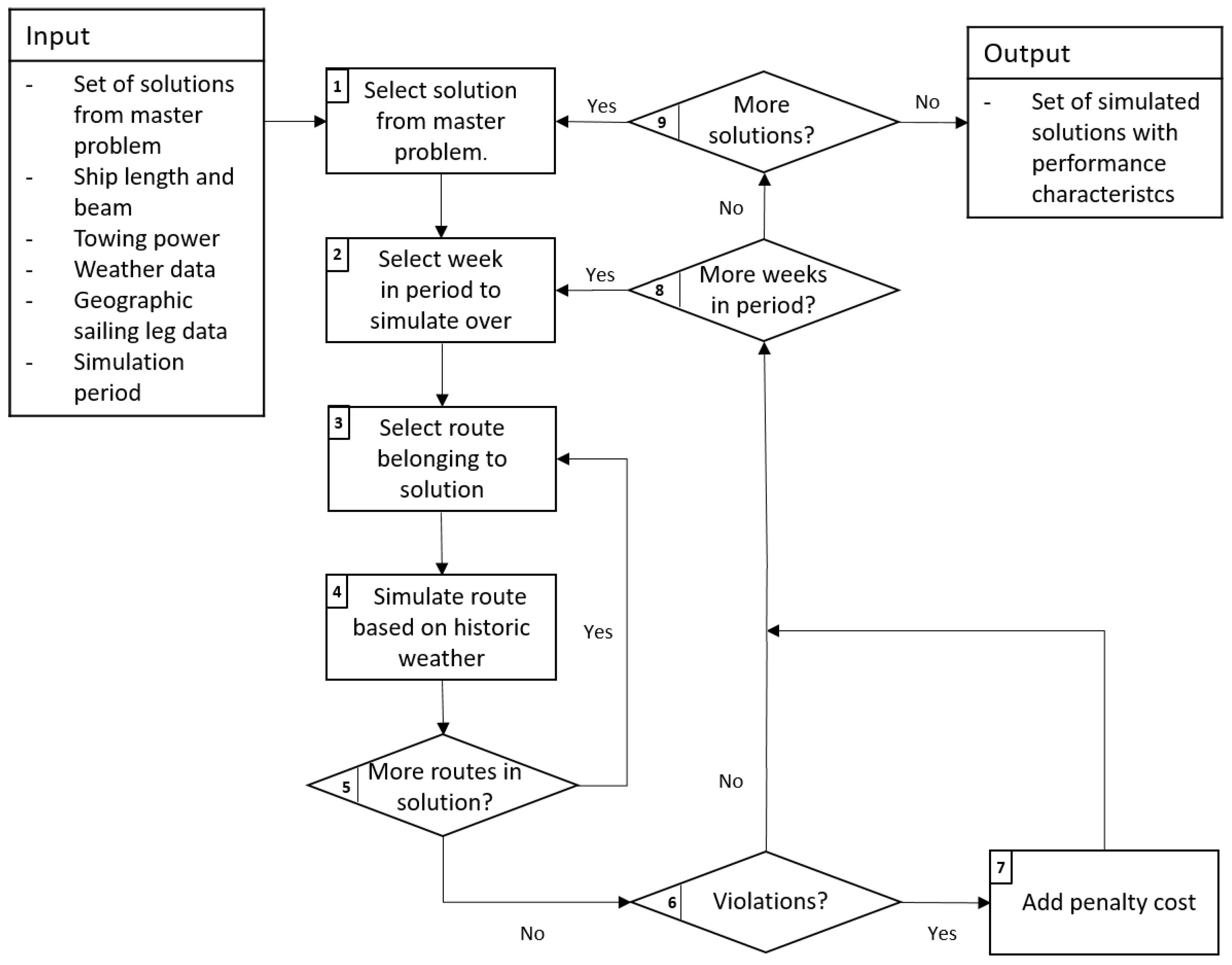
The flow chart in Figure 5 shows the overall simulation process. The input to the simulation model is one (or more) feasible solution(s) from the master problem. In Step 1, the simulation model chooses a solution from the master problem. The week to simulate is chosen in Step 2. In Steps 3–5, all routes in the solution are simulated. Once all routes in the solution are simulated for the given week, synchronization and duration violations are calculated in Step 6. Note that these violations are system-specific, i.e., dependent on the set of routes in the given solution and not only on each route individually. If any violations occur, penalty costs are added to the solution in Step 7. Step 8 checks whether the solution has been simulated for all weeks. Finally, Step 9 ensures that all solutions provided by the optimization model are simulated.
An important element of the simulation model is to penalize duration and synchronization violations. The total penalty cost for a simulated solution is the accumulated penalty costs for all vessels for each week of the simulation period. Hence, route compositions that often incur duration or synchronization violations are receiving a high penalty cost and are less likely to be chosen by the master problem in subsequent iterations.
4.3. Performance-Improving Strategies
Penalizing synchronization and duration violations helps select more robust routes for both mother and daughter vessels, but does not necessarily reflect real-world operations of a feeder network service. In our optimization-simulation model, duration violations propagate from one week to another. In contrast, real-world vessel operators would try to either avoid a delay (e.g., by using more robust routes) or recover from the delay (e.g., by speeding up) before it causes any violations. To further improve the quality of the solutions, we propose two types of performance-improving strategies that mimic real-world operations and are integrated into the solution approach: enhancing the robustness of the routes and recovery from delays.
4.3.1. Enhancing Route Robustness
The first type of strategy tries to enhance the routes’ robustness during the route generation procedure, i.e., before starting the optimization-simulation process. Additional slack (or idle time) is added to some or all of its legs when generating routes. By doing so, a vessel might still be able to synchronize in an ocean hub, even if it has to slow down due to harsh weather. Conversely, adding too much slack can cause excessive waiting times and, as such, increase the operational cost for the vessels. Therefore, determining the amount and place of additional slack while ensuring a sufficient robustness level is an important trade-off to assess. This strategy is comparable to the current practice of airlines where delayed routes can recover at night when no flights are scheduled and the network resets [36].
Similarly, the robustness of the routes can be enhanced by considering seasonality in the schedules. Due to the difference in weather conditions between summer and winter, it might be beneficial to operate dedicated routes for each season. However, the system needs to operate the same fleet of mother and daughter vessels during the whole year, regardless of the season.
4.3.2. Recovery from Delays
The second type of strategy tries to exploit operational flexibility to recover from delays. If weather permits, a vessel can increase its speed to reduce or even eliminate a delay. Fischer et al. [30], for example, show that speed-up can be used as a recovery action when considering disruptions in planning fleet deployment in roll-on roll-off liner shipping. Though speeding-up allows recovering from delays in some cases, it requires increased power output, which in turn will increase fuel consumption and thus bunker costs. The ability to speed-up is limited by the maximum propulsion power of the vessels.
5. Computational Study
The route generation procedure and the simulation model have been implemented in MATLAB R2016b. The master problem is formulated and solved using FICO Xpress 7.9. All computations have been carried out on a PC with a 3.4 GHz Intel Core i7 processor and 32 GB RAM.
5.1. The Short Sea Pioneer Logistics System
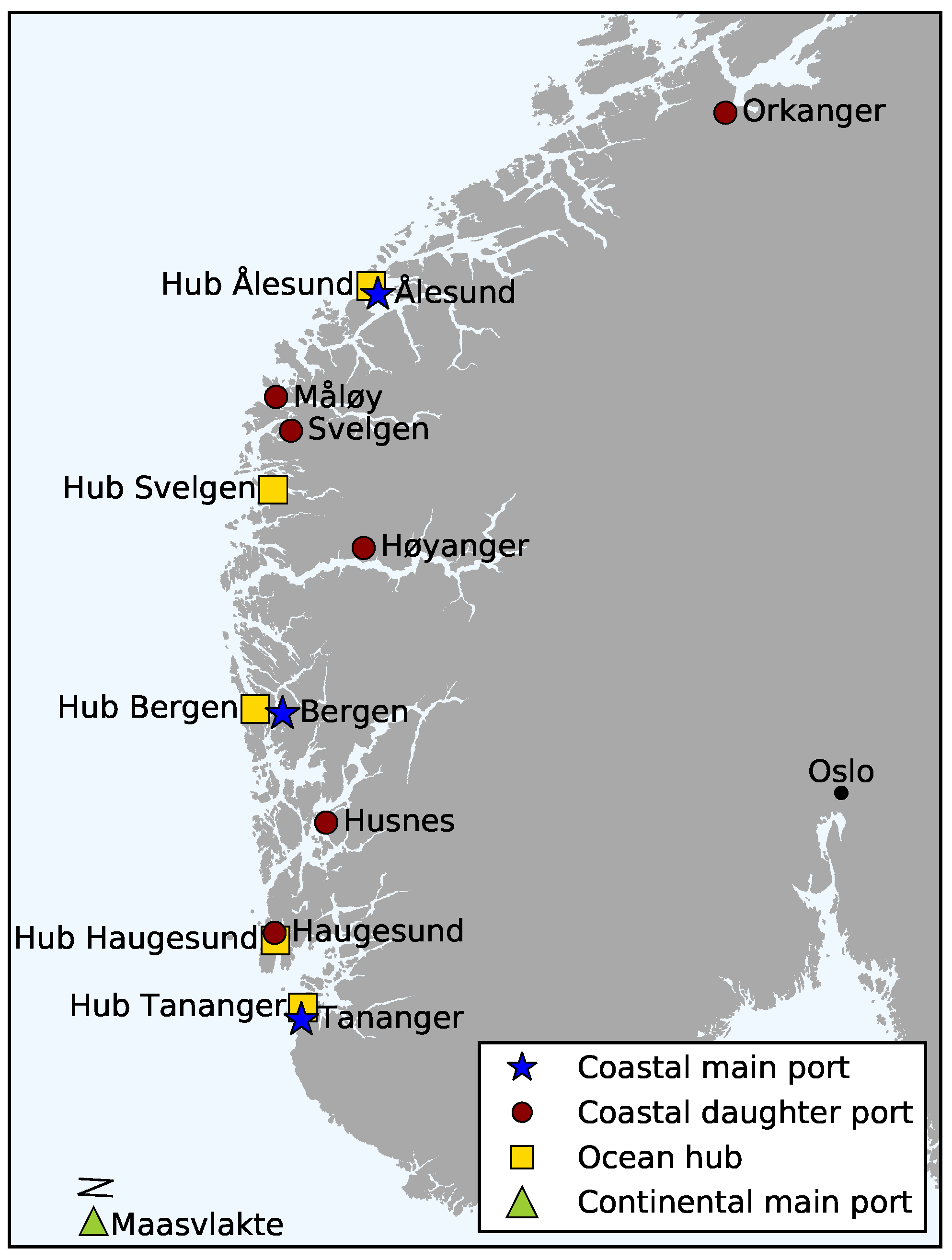
The selection of ports is based on the ports currently served by the case shipping company NorthSea Container Line (NCL), which operates a line for container transportation between the Norwegian west coast and the European continent port located at Maasvlakte in the Netherlands. The candidate hub locations are selected close to major local ports and inshore to have stable weather conditions for the cargo transshipment. The port locations of this case study are illustrated in Figure 6.
The weekly number of containers transported to and from the European continent is based on the number of containers imported and exported in ports along the Norwegian west coast during the first quarter 2016 data [40]. The numbers have been corrected according to NCL’s market share to approximate realistic transportation demand. We refer to Holm et al. [10] for detailed input data.
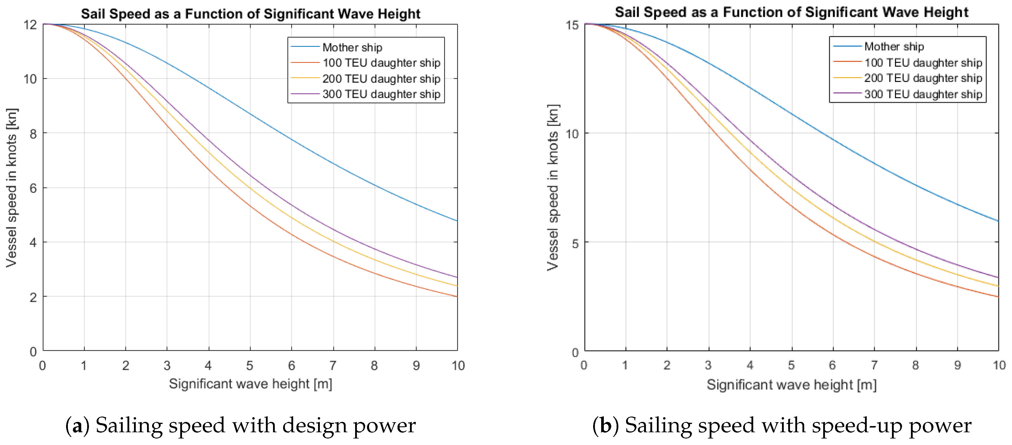
The possible capacities for the daughter vessels are 100, 200, and 300 twenty-foot-equivalent units (TEU). The capacity of the mother vessels is 2500 TEU, which is sufficient to transport the cargo of the whole system. The design speed for all vessels is set to 12 knots.
The relationship between speed and wave height for the mother and three candidate daughter vessel types considered in this experiment is shown in Figure 7. We can see from Figure 7a that at design power, the sailing speed significantly decreases as waves become higher, especially for the daughter vessels. Figure 7b illustrates the same relationship, but for speed-up power that can be used to recover from delays. The power output for speed-up is set to be 125% of design power.
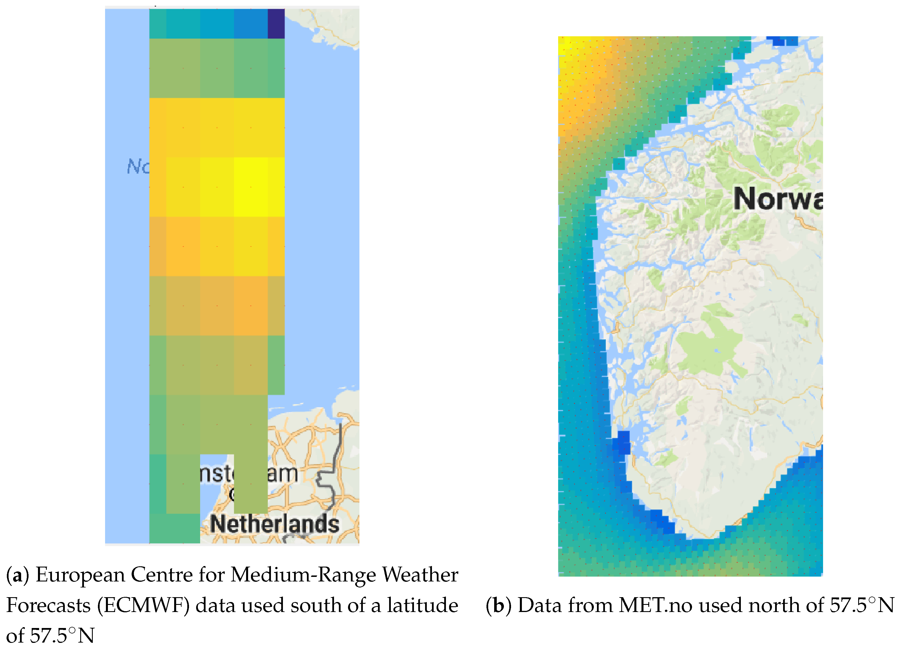
The legs between ports required to simulate sailing speed have been discretized according to container vessel AIS data available from the Norwegian Coastal Administration. Historical wave height data from both the Norwegian Meteorological Institute (MET.no) and the European Centre for Medium-Range Weather Forecasts (ECMWF) is used in the simulations. These data sets provide weather data with a time increment of six hours. Figure 8 shows a visualization of the data grid for both data sources. The data from ECMWF has a resolution of , which is sufficient for the zone between Europe and Norway but not detailed enough for vessels sailing the Norwegian coastline. The data from Norwegian Meteorological Institute offers a better resolution, i.e., and is used for latitudes higher than N. Please note that no wave height data is available inside fjords or very close to land. If a vessel is within these areas, it is assumed to sail at design speed, i.e., 12 knots.
In our simulations, we use data of two successive years (2000 and 2001). To make the simulation by weeks easier, we assume that the length of each month is exactly four weeks, resulting in a total of 96 weeks to simulate. The winter season is defined as lasting from October to March, and the summer season lasts from April to September.
5.2. Runtime Considerations
The runtime of the optimization-simulation framework mainly depends on the number of iterations needed for the framework to converge to a solution. To speed up this process, we can reduce the number of times to run the optimization model by returning multiple feasible solutions for simulation instead of only the optimal solution. This has the advantage of possibly simulating the solution that performs best under uncertainty at early iterations. On the other hand, extracting too many solutions implies simulating solutions that may never be needed. Thus, it would be interesting to study the trade-off between the number of solutions extracted in each iteration and the number of iterations of the optimization-simulation framework.
We extract the n best solutions found while solving the master problem. The results for the convergence speed of the solution method for different values of n are presented in Table 1. The first column indicates the maximum number of extracted solutions n in each iteration. The column Itr. needed states how many times the master problem has been solved, i.e., the number of iterations. The third column, Route Gen. Time, is the time needed to generate the routes. Note that this time is constant, as the routes are only generated once. The total time spent by Xpress to solve the master problems is given in column Opt. Time, whereas the total time used by MATLAB to simulate the solutions is given in column Sim. Time. Column Total Time shows the total runtime spent by the solution approach. The last column, Solutions Simulated, contains the total number of simulated solutions.
As can be seen from Table 1, the number of iterations of solving the master problem decreases with higher values of n. In contrast, the time needed to simulate all solutions increases by n. For our case, we select for which the best total time is obtained. Finally, we point out that the approach is not sensitive to n when considering the solution quality. The same best solution is found for all different values of n.
5.3. Determining Global Estimated Optimal Routes
In this section, we analyze the route networks obtained using the solution method. We first describe the different performance-improving strategies, before discussing the solutions produced by our method.
5.3.1. Performance-Improving Strategies
We combine the optimization-simulation solution method with different performance-improving strategies to impose additional robustness and exploit operational flexibility. The different strategies are listed in Table 2 and are explained in more detail below.
We test three different performance-enhancing strategies for enhancing the robustness of the routes and one strategy for recovery from delays. The Slack 10% and the Realistic strategies are implemented as part of the route generation procedure. The Slack 10% strategy is characterized by calculating the sailing time along a leg (based on design speed) and then adding 10% additional sailing to immunize the route against delays. While adding robustness to a route, this strategy may result in considerable amounts of unnecessary idle time in the schedule. The Realistic strategy tries to account for the fact that particular sailing legs are more likely to be subject to delays than others. Sailing speeds along the different legs are first simulated using weather data from 1998 to 2000. To further improve robustness, the resulting average sailing time on each leg is then increased by an additional 5%.
With the Seasonal strategy, the routes sailed by the vessels are allowed to change for each season. We distinguish here between the summer season and winter season. The seasonal routes are obtained by solving the simulation-optimization framework for each season with a set of routes based on design speed. Note that the same fleet has to be used in all seasons.
The Speed-up strategy is part of the simulation model. This strategy allows delayed vessels to increase their speed by increasing their power output. Mother and daughter vessels speed-up independently according to their routes, but the conditions for when they do so are slightly different. A mother vessel will try to speed-up once it is more than one hour delayed compared to its generated route. Increased speed will be maintained until the vessel is no longer delayed. Daughter vessels usually have a certain amount of idle time included in their schedules, e.g., waiting for the mother vessel to arrive in an ocean hub. The daughter vessel starts to speed-up as soon as the remaining idle time falls below a given threshold (for the case study, this is set to one hour) and will continue to sail at increased speed until it has up to two hours idle time available. However, a daughter vessel will never speed-up to get more than its original amount of idle time.
The Combined strategy applies realistic, speed-up, and seasonal strategies simultaneously. The realistic sailing times used in the combined strategy are calculated separately for each season during the preliminary simulation of sailing time. This implies that more absolute slack will be added in the winter season than in the summer season.
5.3.2. Best Routes with and without Weather Uncertainty
We first solve the problem deterministically and use its solution as a benchmark when comparing the solutions considering weather uncertainty. For the deterministic case, the solution using daughter vessels with a capacity of 300 TEU has the lowest total weekly cost with an objective function value of 457,800 USD. Two mother vessels and two daughter vessels are deployed in this optimal solution, as shown in Figure 9. In particular, the main route visits two ocean hubs at Tananger and Haugesund, as well as the main port at Tananger. The hub Haugesund is the northernmost port served by the main route and is therefore visited only once. The mother vessel is more expensive in terms of bunker cost and port visits, which causes the model to select a short main route.
We then solve the network design problem using our optimization-simulation method, applying each of the performance-improving strategies separately. In all best solutions, two mother vessels and two daughter vessels are deployed. However, the solution without the performance-improving strategy deploys smaller daughter vessels than other solutions. Table 3 summarizes the results for the different performance-improving strategies. The cost of the best solutions is compared to the cost of the best deterministic solution, where 100% representing the cost of the deterministic solution. In this comparison, the penalty costs added by the simulation model are excluded as they are fictional and only used to identify low-performing solutions. However, the increased costs due to speeding up are included. This comparison facilitates evaluating the solution quality since the deterministic solution is obtained under ideal weather conditions and, thus, can be considered as a lower bound. Table 3 also shows important performance characteristics for the different solutions, such as the total number and accumulated time (in hours) of both duration and synchronization violations. It also reports the total amount of planned idle time included in the selected routes and how much time this idle time is used to recover from incurred delays. The last column indicates the daughter vessel size of the solutions.
All obtained solutions result in a slight increase in operational costs compared to the deterministic solution, where the Combined strategy gives the lowest operational cost with an increase of only 1.2%. Only one duration violation occurs with a negligible magnitude. The number of synchronization violations and the related magnitude is also significantly lower than for other strategies. The utilization of idle time is also low, implying that the vessels usually keep the estimated arrival times set up in the route generation procedure. As such, the solution obtained when using the combined performance-improving strategy is quite robust without increasing the cost level by much. Note that the solution resulting from not using a performance-improving strategy does not incur any duration violation but is exposed to many synchronization violations. The solution includes a lot of idle time, a large share of which needs to be used for sailing to recover from delays.
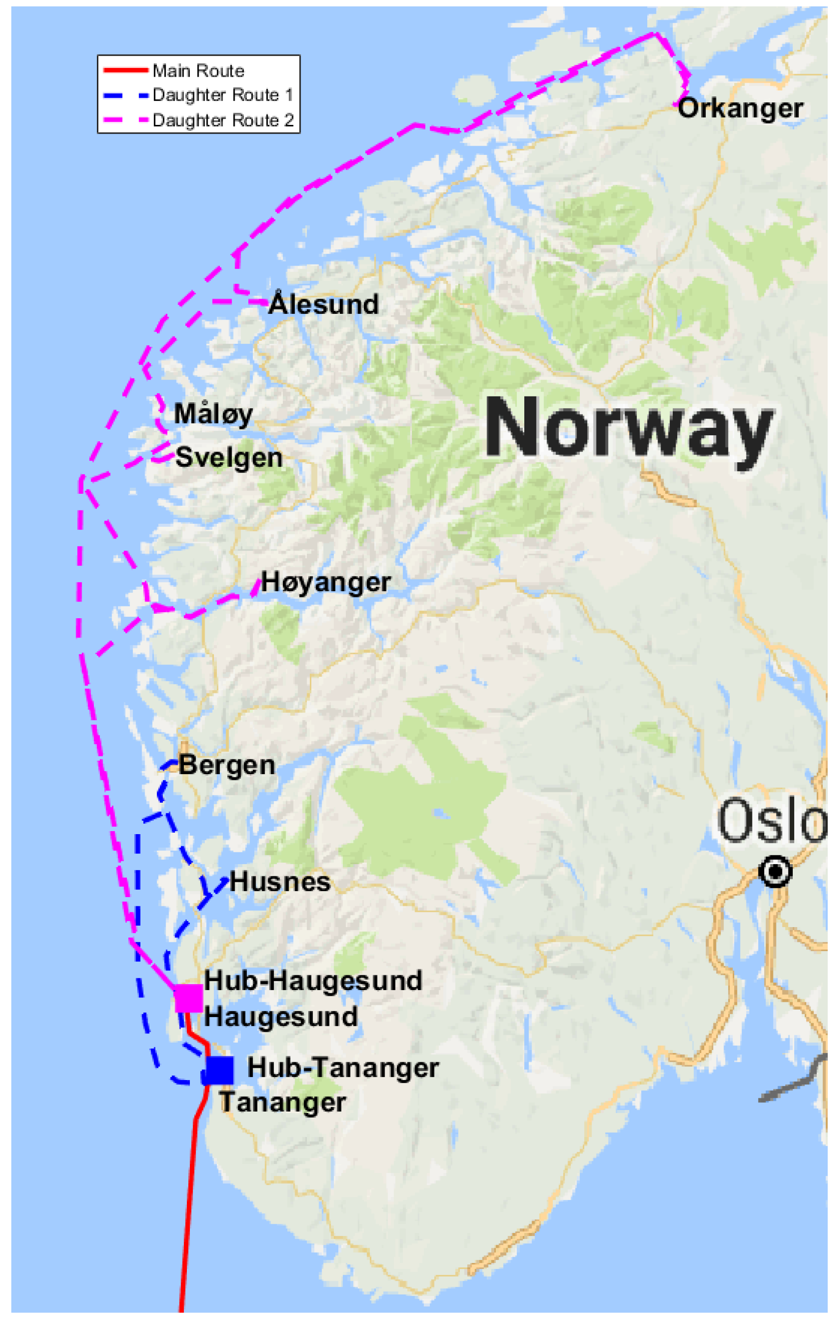
Figure 10 shows the optimal seasonal routes for the Combined strategy. The solid red line is the main route that continues further south to Maasvlakte port. The blue and pink dashed lines are daughter routes 1 and 2, respectively. The corresponding ocean hubs are marked as squares.
As seen in Figure 10, the main route extends further north in the winter than during the summer season. Compared to a daughter vessel, a mother vessel is more expensive in terms of bunker and port costs. By having a mother vessel sailing further north, the daughter vessels can reduce their total sailing distance, resulting in planned idle time. This is beneficial during the winter season since the weather conditions are rougher, and a greater buffer against delays is needed to avoid duration violations. Conversely, during the summer season, the weather conditions are better, resulting in a shorter main route with corresponding longer daughter routes to reduce operational cost.
5.3.3. Analyzing the Best Deterministic Solution
The best deterministic solution is slightly cheaper than all solutions found by the solution triggered feedback approach. However, these cost savings come at the expense of a lack of robustness for harsh weather conditions. Table 4 provides the performance characteristics for simulating the optimal deterministic solution under weather conditions without any performance-improving strategy.
In particular, the high number of duration violations renders the best deterministic solution infeasible in practice. While almost all of the planned idle time is used for sailing to mitigate delays, the system is still unable to recover. The poor performance of the optimal deterministic solution clearly shows the importance of taking into account weather uncertainty. All solutions found the using optimization-simulation approach (see Table 3) perform significantly better, while being less than 3% more expensive. The solution from the Combined strategy for example, reduces the number of duration violations from 277 to 1 and the duration magnitude from 45,429 h to 0.7 h, while the costs only increase by 1.2%.
Pushing the analysis further, we simulate the best deterministic solution with the Speed-up strategy. This combination results in a cost increase of 2.2%, which is due to the higher fuel consumption from the required speed-ups. However, the number of duration violations is reduced from 277 to 28, and the number of synchronization violation is reduced from 194 to 181. Even though these are significant improvements, the solution still performs much worse than the solutions found by the optimization-simulation method.
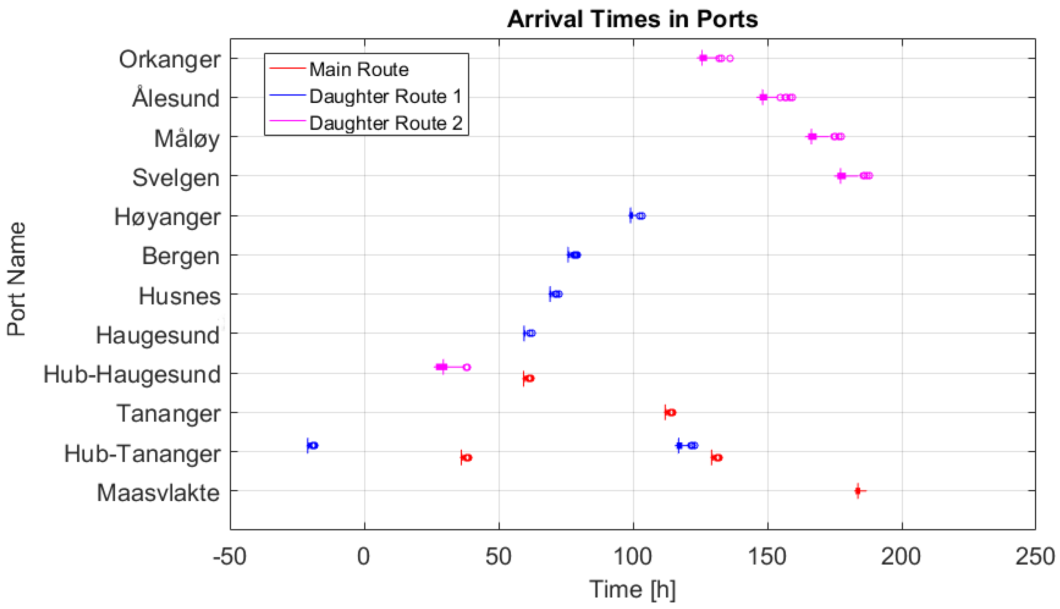
In another analysis, we consider another criterion of a well-performing solution. It consists of measuring the stability of arrival times, which translates directly into predicting future arrivals and maintaining a given schedule. For the Combined-strategy solution, the arrival times for the summer and winter routes are presented in Figure 11 and Figure 12. The mother vessels are scheduled to depart from the main continental port at time zero. The arrival times for all vessels refer to this departure time.
The small vertical line represents the median arrival time. The width of each box corresponds to the interquartile range () defined by the first and third quartile, and accounts for 50% of all port arrivals in the simulation period. The left and right whiskers capture all arrival times within . Arrival times outside this range are considered outliers and represented with circles.
For both seasons, arrival times are mostly within relatively small intervals, particularly for the main route and daughter route 1. The longer daughter route 2 is slightly more prone to variations in arrival time, especially during the winter season, although this route is considerably shortened during this season (see Figure 10). Still, these varying arrival times do not affect synchronization with the mother vessel at ocean hubs (except Bergen) because daughter vessel 2 always arrives first anyway (with one exception).
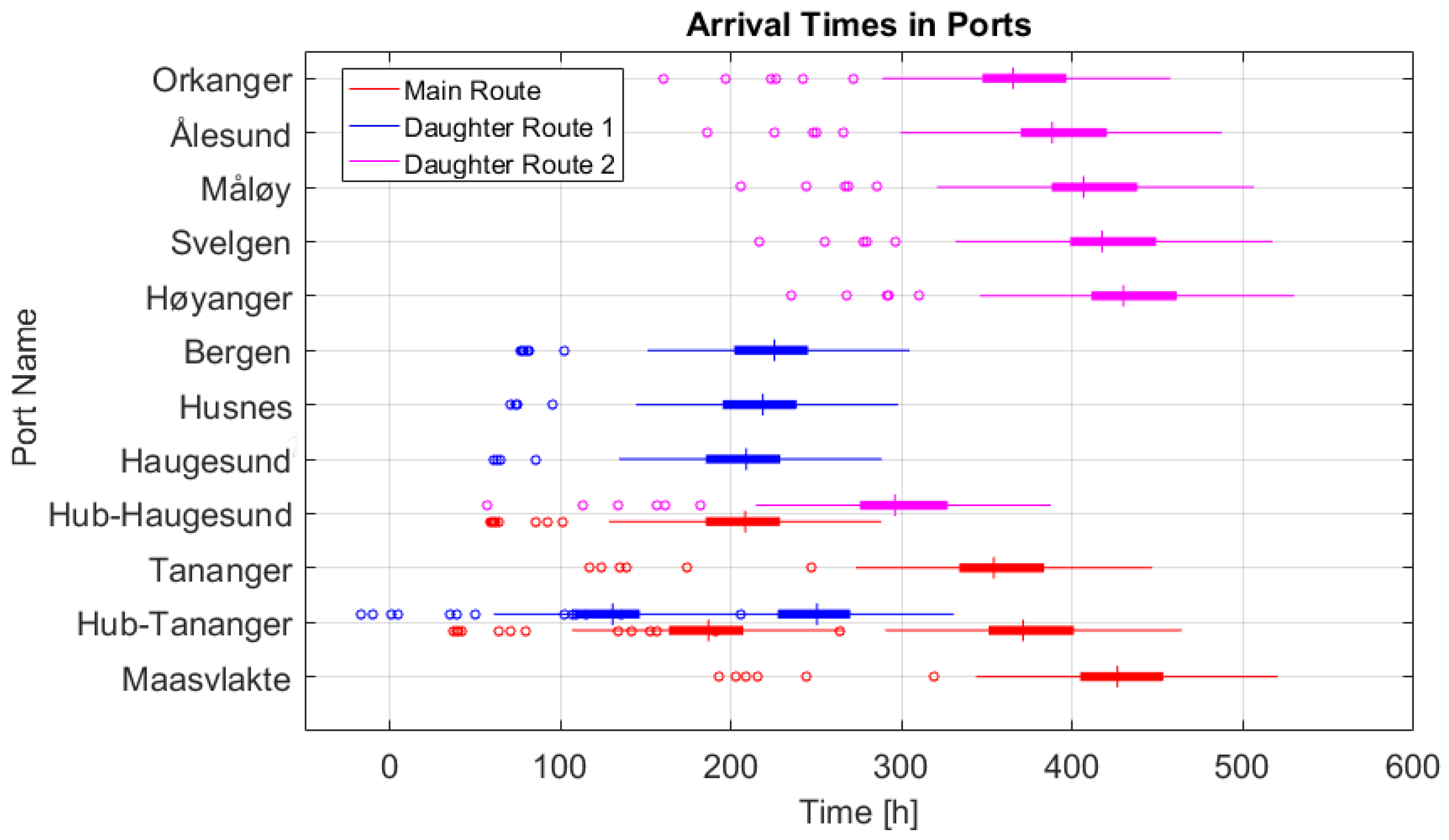
Figure 13 presents the arrival times for the deterministic solution. Here, we observe much wider intervals for different arrival times. For example, about 50% of all arrivals at the main continental port in Maasvlakte happen approximately 48 h around the median arrival time. This median arrival time of the mother vessel is also about 100 h after the end of the planned two-week route due to a large number of duration violations. Moreover, Figure 13 shows that the deterministic solution is very sensitive to weather uncertainty, causing arrival times to vary a lot. Therefore, the deterministic solution is not applicable in a real-world setting and should be discarded in favor of the solution from the Combined-strategy. These results highlight once more the need for considering the weather uncertainty in designing the short-sea feeder network considered in this paper.
6. Concluding Remarks
In this paper, we study the problem of designing a short-sea liner network with transshipment at sea under uncertain weather conditions and propose an iterative solution method that combines optimization and simulation. In the deterministic optimization step, we select routes for both mother and daughter vessels that minimize the cost of operating the logistics system. These routes are then evaluated using a discrete event simulation model. Solutions that are not performing well in the simulations are penalized in the objective function in subsequent iterations of the optimization model to reduce their attractiveness. The steps of selecting routes in the optimization model and simulating them continue until no new (not simulated) solution is selected. The computational study performed on a case based on real-world data shows that our solution method provides solutions for the system with a good trade-off between operational cost and robustness.
The results show that weather uncertainty can severely impact the synchronization of the routes and should be taken into account in the design phase of the logistics system. The optimization-simulation approach, especially when using different performance-improving strategies, finds robust solutions at only a small operational cost increase. The solution method has been applied to a short-sea feeder network design problem in this paper, but it should be straightforward to apply to other related problems.
Author Contributions
Conceptualization, K.F. and P.S.; methodology, C.A.B.M., M.B.H., K.F. and P.S.; software, C.A.B.M. and M.B.H.; validation, C.A.B.M., M.B.H., K.F. and P.S.; formal analysis, C.A.B.M. and M.B.H.; investigation, C.A.B.M. and M.B.H.; writing—original draft preparation, C.A.B.M. and M.B.H.; writing—review and editing, M.K.M., K.F. and P.S.; visualization, C.A.B.M. and M.B.H.; supervision, K.F. and P.S.; project administration, K.F. and P.S. All authors have read and agreed to the published version of the manuscript. Authors contributed equally to this work.
Funding
This research received no external funding.
Conflicts of Interest
The authors declare no conflict of interest.
References
- Brouer, B.D.; Karsten, C.V.; Pisinger, D. Optimization in liner shipping. 4OR 2017, 15, 1–35. [Google Scholar] [CrossRef]
- Christiansen, M.; Fagerholt, K.; Nygreen, B.; Ronen, D. Maritime Transportation. In Transportation; Elsevier: Amsterdam, The Netherlands, 2007; pp. 189–284. [Google Scholar] [CrossRef]
- Haram, H.K.; Hov, I.B.; Caspersen, E. Potensiale og Virkemidler for Overføring av Gods Fra Veg- Til Sjøtransport. Available online: https://www.toi.no/getfile.php?mmfileid=41079 (accessed on 27 July 2020).
- Goel, A. A roadmap for sustainable freight transport. In Methods of Multicriteria Decision Theory and Applications; Shaker: Maastricht, Germany, 2009; pp. 47–56. [Google Scholar]
- Norwegian Ministry of Transport and Communications. Nasjonal Transportplan 2014–2023. Available online: https://www.regjeringen.no/no/dokumenter/meld-st-26-20122013/id722102/ (accessed on 27 July 2020).
- Norwegian Ministry of Transport and Communications. Nasjonal Transportplan 2018–2029. Available online: https://www.regjeringen.no/no/dokumenter/meld.-st.-33-20162017/id2546287/ (accessed on 27 July 2020).
- NCE Maritime Clean Tech. Short Sea Pioneer the New Way of Transporting Goods at Sea. Available online: https://maritimecleantech.no/wp-content/uploads/2017/01/SSP-folder.pdf (accessed on 27 July 2020).
- NCE Maritime Clean Tech. Short Sea Pioneer. Available online: https://maritimecleantech.no/project/short-sea-pioneer-2 (accessed on 27 July 2020).
- Stensvold, T. Slik skal ny 2-i-1-løsning Flytte Mer Gods Fra Vei Til Sjø. Available online: http://www.tu.no/artikler/slik-skal-ny-2-i-1-losning-flytte-mer-gods-fra-vei-til-sjo/223103 (accessed on 27 July 2020).
- Holm, M.B.; Medbøen, C.A.B.; Fagerholt, K.; Schütz, P. Shortsea liner network design with transhipments at sea: A case study from Western Norway. Flex. Serv. Manuf. J. 2018, 31, 598–619. [Google Scholar] [CrossRef]
- Brouer, B.D.; Alvarez, J.F.; Plum, C.E.M.; Pisinger, D.; Sigurd, M.M. A Base Integer Programming Model and Benchmark Suite for Liner-Shipping Network Design. Transp. Sci. 2014, 48, 281–312. [Google Scholar] [CrossRef] [Green Version]
- Meng, Q.; Wang, S. Liner shipping service network design with empty container repositioning. Transp. Res. Part E Logist. Transp. Rev. 2011, 47, 695–708. [Google Scholar] [CrossRef]
- Reinhardt, L.B.; Pisinger, D. A branch and cut algorithm for the container shipping network design problem. Flex. Serv. Manuf. J. 2012, 24, 349–374. [Google Scholar] [CrossRef] [Green Version]
- Karsten, C.V.; Brouer, B.D.; Pisinger, D. Competitive Liner Shipping Network Design. Comput. Oper. Res. 2017, 87, 125–136. [Google Scholar] [CrossRef] [Green Version]
- Balakrishnan, A.; Karsten, C.V. Container shipping service selection and cargo routing with transshipment limits. Eur. J. Oper. Res. 2017, 263, 652–663. [Google Scholar] [CrossRef] [Green Version]
- Msakni, M.K.; Fagerholt, K.; Meisel, F.; Lindstad, E. Analyzing different designs of liner shipping feeder networks: A case study. Transp. Res. Part E Logist. Transp. Rev. 2020, 134, 101839. [Google Scholar] [CrossRef]
- Fadda, P.; Fancello, G.; Mancini, S.; Pani, C.; Serra, P. Design and optimisation of an innovative two-hub-and-spoke network for the Mediterranean short-sea-shipping market. Comput. Ind. Eng. 2020, 149, 106847. [Google Scholar] [CrossRef]
- Akbar, A.; Aasen, A.K.A.; Msakni, M.K.; Fagerholt, K.; Lindstad, E.; Meisel, F. An economic analysis of introducing autonomous ships in a short-sea liner shipping network. Int. Trans. Oper. Res. 2020. [Google Scholar] [CrossRef] [Green Version]
- Meng, Q.; Wang, S.; Andersson, H.; Thun, K. Containership routing and scheduling in liner shipping: Overview and future research directions. Transp. Sci. 2014, 48, 265–280. [Google Scholar] [CrossRef] [Green Version]
- Christiansen, M.; Hellsten, E.; Pisinger, D.; Sacramento, D.; Vilhelmsen, C. Liner shipping network design. Eur. J. Oper. Res. 2019. [Google Scholar] [CrossRef]
- Agarwal, R.; Ergun, Ö. Ship Scheduling and Network Design for Cargo Routing in Liner Shipping. Transp. Sci. 2008, 42, 175–196. [Google Scholar] [CrossRef]
- Andersson, H.; Duesund, J.M.; Fagerholt, K. Ship routing and scheduling with cargo coupling and synchronization constraints. Comput. Ind. Eng. 2011, 61, 1107–1116. [Google Scholar] [CrossRef]
- Drexl, M. Synchronization in Vehicle Routing—A Survey of VRPs with Multiple Synchronization Constraints. Transp. Sci. 2012, 46, 297–316. [Google Scholar] [CrossRef] [Green Version]
- Wang, S.; Meng, Q. Liner ship route schedule design with sea contingency time and port time uncertainty. Transp. Res. Part B Methodol. 2012, 46, 615–633. [Google Scholar] [CrossRef]
- Song, D.P.; Li, D.; Drake, P. Multi-objective optimization for planning liner shipping service with uncertain port times. Transp. Res. Part E Logist. Transp. Rev. 2015, 84, 1–22. [Google Scholar] [CrossRef]
- Li, C.; Qi, X.; Song, D. Real-time schedule recovery in liner shipping service with regular uncertainties and disruption events. Transp. Res. Part B Methodol. 2016, 93, 762–788. [Google Scholar] [CrossRef]
- Ng, M.; Lin, D.Y. Fleet deployment in liner shipping with incomplete demand information. Transp. Res. Part E Logist. Transp. Rev. 2018, 116, 184–189. [Google Scholar] [CrossRef]
- Lo, H.K.; An, K.; Lin, W. Ferry service network design under demand uncertainty. Transp. Res. Part E Logist. Transp. Rev. 2013, 59, 48–70. [Google Scholar] [CrossRef]
- An, K.; Lo, H.K. Two-phase stochastic program for transit network design under demand uncertainty. Transp. Res. Part B Methodol. 2016, 84, 157–181. [Google Scholar] [CrossRef]
- Fischer, A.; Nokhart, H.; Olsen, H.; Fagerholt, K.; Rakke, J.G.; Stålhane, M. Robust planning and disruption management in roll-on roll-off liner shipping. Transp. Res. Part E Logist. Transp. Rev. 2016, 91, 51–67. [Google Scholar] [CrossRef] [Green Version]
- Castilla-Rodríguez, I.; Expósito-Izquierdo, C.; Melián-Batista, B.; Aguilar, R.M.; Moreno-Vega, J.M. Simulation-optimization for the management of the transshipment operations at maritime container terminals. Expert Syst. Appl. 2020, 139, 112852. [Google Scholar] [CrossRef]
- Layeb, S.B.; Jaoua, A.; Jbira, A.; Makhlouf, Y. A simulation-optimization approach for scheduling in stochastic freight transportation. Comput. Ind. Eng. 2018, 126, 99–110. [Google Scholar] [CrossRef]
- Poeting, M.; Rau, J.; Clausen, U.; Schumacher, C. A combined simulation optimization framework to improve operations in parcel logistics. In Proceedings of the 2017 Winter Simulation Conference (WSC), Las Vegas, NV, USA, 3–6 December 2017. [Google Scholar] [CrossRef]
- Acar, Y.; Kadipasaoglu, S.N.; Day, J.M. Incorporating uncertainty in optimal decision making: Integrating mixed integer programming and simulation to solve combinatorial problems. Comput. Ind. Eng. 2009, 56, 106–112. [Google Scholar] [CrossRef]
- Crainic, T.G.; Perboli, G.; Rosano, M. Simulation of intermodal freight transportation systems: A taxonomy. Eur. J. Oper. Res. 2018, 270, 401–418. [Google Scholar] [CrossRef]
- Brouer, B.D.; Dirksen, J.; Pisinger, D.; Plum, C.E.; Vaaben, B. The Vessel Schedule Recovery Problem (VSRP)—A MIP model for handling disruptions in liner shipping. Eur. J. Oper. Res. 2013, 224, 362–374. [Google Scholar] [CrossRef]
- Irnich, S. Resource extension functions: Properties, inversion, and generalization to segments. OR Spectr. 2008, 30, 113–148. [Google Scholar] [CrossRef]
- DNV GL. Environmental Conditions and Environmental Loads. Recommended Practice DNV-RP-C205. Available online: https://rules.dnvgl.com/docs/pdf/dnv/codes/docs/2010-10/rp-c205.pdf (accessed on 2 April 2020).
- Van den Boom, H.; Van der Hout, I.; Flikkema, M. Speed-power performance of ships during trials and in service. In Proceedings of the SNAME, Athens, Greece, 17–18 September 2008. [Google Scholar]
- Statistics Norway. Maritime Transport. Available online: https://www.ssb.no/en/statbank/table/03648/ (accessed on 27 July 2020).
Figure 1.
An example of the short sea pioneer (SSP) logistics system [10] composed of one main route and three daughter routes. The main route serves the continental port, Maasvlakte, a large Norwegian port in Bergen, and three ocean hubs. All daughter routes depart from ocean hubs and serve local Norwegian ports.

Figure 2.
An example to show duration and synchronization violations due to harsh weather. The mother vessel has to wait for 10 h in ocean hub 1s, causing a synchronization violation and a duration violation of five hours.
Figure 2.
An example to show duration and synchronization violations due to harsh weather. The mother vessel has to wait for 10 h in ocean hub 1s, causing a synchronization violation and a duration violation of five hours.

Figure 3.
An overview of the optimization-simulation framework. From input data, the routes are generated. The master problem and the simulation model are iteratively solved until no new solution is found.
Figure 3.
An overview of the optimization-simulation framework. From input data, the routes are generated. The master problem and the simulation model are iteratively solved until no new solution is found.

Figure 4.
Illustration of a leg. The vessel changes direction at the waypoints and the speed is updated at every observation point.
Figure 4.
Illustration of a leg. The vessel changes direction at the waypoints and the speed is updated at every observation point.

Figure 5.
Flow chart of the simulation model. The solutions provided by the master problem are simulated week-by-week over a long period using historical data. When a violation is detected, a penalty cost is added to the operational costs of the solution.
Figure 5.
Flow chart of the simulation model. The solutions provided by the master problem are simulated week-by-week over a long period using historical data. When a violation is detected, a penalty cost is added to the operational costs of the solution.

Figure 6.
A map showing ports considered in the case study. The possible ocean hubs are represented with yellow squares.
Figure 6.
A map showing ports considered in the case study. The possible ocean hubs are represented with yellow squares.

Figure 7.
Impact of significant wave heights on the sailing speed for the fleet of vessels considered in the experimentation.
Figure 7.
Impact of significant wave heights on the sailing speed for the fleet of vessels considered in the experimentation.

Figure 8.
Data grid with time series observation on each cell used for the weather simulation.

Figure 9.
The optimal routes for the Short Sea Pioneer (SSP) deterministic version. The mother route visits two hub ports that are connected to two daughter routes.
Figure 9.
The optimal routes for the Short Sea Pioneer (SSP) deterministic version. The mother route visits two hub ports that are connected to two daughter routes.

Figure 10.
The difference between the summer and winter solutions when using the combined strategy. The main route sails further north in the winter season due to rough weather conditions.
Figure 10.
The difference between the summer and winter solutions when using the combined strategy. The main route sails further north in the winter season due to rough weather conditions.

Figure 11.
A box and whisker plot of the arrival times for the summer season of the Combined-strategy solution.
Figure 11.
A box and whisker plot of the arrival times for the summer season of the Combined-strategy solution.

Figure 12.
A box and whisker plot of the arrival times for the winter season of the Combined-strategy solution.
Figure 12.
A box and whisker plot of the arrival times for the winter season of the Combined-strategy solution.

Figure 13.
A box and whisker plot of the arrival times of deterministic solution.


Table 1.
Runtime (in seconds) for the solution approach with different values of n.
| n | Itr. needed | Route Gen. Time | Opt. Time | Sim. Time | Total Time | Solutions Simulated |
|---|---|---|---|---|---|---|
| 1 | 75 | 94 | 2855 | 131 | 3080 | 75 |
| 5 | 19 | 94 | 771 | 149 | 1014 | 89 |
| 10 | 13 | 94 | 510 | 182 | 786 | 113 |
| 20 | 9 | 94 | 390 | 246 | 730 | 157 |
| 50 | 7 | 94 | 405 | 473 | 972 | 297 |
| 100 | 6 | 94 | 393 | 573 | 1060 | 494 |
Table 2.
List of applied performance-improving strategies.
| Strategy | Category | Description |
|---|---|---|
| None | - | No performance-improving strategy is applied. |
| Slack 10% | Route robustness | 10% slack is added on each sailing leg. |
| Realistic | Route robustness | Simulated sailing times with additional 5% extra slack. |
| Seasonal | Route robustness | Tailor-made winter and summer schedules are used. |
| Speed-up | Recovery | vessels can speed-up to reduce delays. |
| Combined | Route robustness & recovery | Realistic, Speed-Up, and Seasonal strategies are applied. |
Table 3.
Performance characteristics for the different solutions.
| Strategy | Cost [%] | Dur. Viol. | Dur. Mag. | Sync. Viol. | Sync. Mag. | Idle Time | Idle Use [%] | Vessel Size |
|---|---|---|---|---|---|---|---|---|
| None | 102.1 | 0 | 0 | 200 | 1958 | 219 | 14.8 | 200 |
| Slack 10% | 101.4 | 4 | 18.7 | 61 | 450 | 171 | 3.9 | 300 |
| Realistic | 101.4 | 4 | 17.1 | 52 | 319 | 162 | 2.5 | 300 |
| Seasonal | 101.5 | 3 | 4.3 | 204 | 1859 | 180 | 17.3 | 300 |
| Speed-up | 102.8 | 2 | 4.1 | 125 | 927 | 188 | 8.9 | 300 |
| Combined | 101.2 | 1 | 0.7 | 21 | 192 | 160 | 1.8 | 300 |
Table 4.
Performance characteristics for the best deterministic solution.
| Cost [%] | Dur. Viol. | Dur. Mag. | Sync. Viol. | Sync. Mag. | Idle Time | Idle Use [%] | Vessel Size |
|---|---|---|---|---|---|---|---|
| 100 | 277 | 45,429 | 194 | 14,332 | 192 | 82.5 | 300 |
Publisher’s Note: MDPI stays neutral with regard to jurisdictional claims in published maps and institutional affiliations. |
© 2020 by the authors. Licensee MDPI, Basel, Switzerland. This article is an open access article distributed under the terms and conditions of the Creative Commons Attribution (CC BY) license (http://creativecommons.org/licenses/by/4.0/).
Share and Cite
MDPI and ACS Style
Medbøen, C.A.B.; Holm, M.B.; Msakni, M.K.; Fagerholt, K.; Schütz, P. Combining Optimization and Simulation for Designing a Robust Short-Sea Feeder Network. Algorithms 2020, 13, 304. https://0-doi-org.brum.beds.ac.uk/10.3390/a13110304
AMA Style
Medbøen CAB, Holm MB, Msakni MK, Fagerholt K, Schütz P. Combining Optimization and Simulation for Designing a Robust Short-Sea Feeder Network. Algorithms. 2020; 13(11):304. https://0-doi-org.brum.beds.ac.uk/10.3390/a13110304
Chicago/Turabian StyleMedbøen, Carl Axel Benjamin, Magnus Bolstad Holm, Mohamed Kais Msakni, Kjetil Fagerholt, and Peter Schütz. 2020. "Combining Optimization and Simulation for Designing a Robust Short-Sea Feeder Network" Algorithms 13, no. 11: 304. https://0-doi-org.brum.beds.ac.uk/10.3390/a13110304
Note that from the first issue of 2016, this journal uses article numbers instead of page numbers. See further details here.