Latency-Bounded Target Set Selection in Signed Networks


1
Dipartimento di Matematica, Università degli Studi di Roma “Tor Vergata”, 00133 Roma, RM, Italy
2
Gran Sasso Science Institute, 67100 L’Aquila, Italy
*
Author to whom correspondence should be addressed.
Algorithms 2020, 13(2), 32; https://0-doi-org.brum.beds.ac.uk/10.3390/a13020032
Submission received: 22 December 2019
/
Revised: 27 January 2020
/
Accepted: 27 January 2020
/
Published: 29 January 2020
(This article belongs to the Special Issue Approximation Algorithms for NP-Hard Problems)
Abstract
:It is well-documented that social networks play a considerable role in information spreading. The dynamic processes governing the diffusion of information have been studied in many fields, including epidemiology, sociology, economics, and computer science. A widely studied problem in the area of viral marketing is the target set selection: in order to market a new product, hoping it will be adopted by a large fraction of individuals in the network, which set of individuals should we “target” (for instance, by offering them free samples of the product)? In this paper, we introduce a diffusion model in which some of the neighbors of a node have a negative influence on that node, namely, they induce the node to reject the feature that is supposed to be spread. We study the target set selection problem within this model, first proving a strong inapproximability result holding also when the diffusion process is required to reach all the nodes in a couple of rounds. Then, we consider a set of restrictions under which the problem is approximable to some extent.
1. Introduction
The study of diffusion processes is a widely investigated topic in the complex networks setting. It aims at analyzing how local interactions among nearby nodes may lead to the diffusion, possibly over the whole network, of some feature (opinion/information/disease) starting from a limited set of initiator (or seed) nodes. The problem known as Influence Maximization has been introduced by Domingos and Richardson [1,2] for the design of viral marketing campaigns on social networks by using a small (let us say, given) number of initiators (for example by providing a limited set of people free samples of a product to be merchandised), starting from which a cascade is triggered maximizing the overall spreading of information (see also [3,4,5,6,7,8,9]). Dually, the target set selection problem aims at finding out a minimum size set of initiators able to spread the feature over the whole network [3,10,11,12,13,14,15,16,17] or over a large (let us say, given) portion of the network; such a set of initiators is called a target set.
Diffusion processes are usually modeled by graphs in which each vertex may be in one out of two states: informed or unaware. Initially, only nodes in a given set are informed, while all the others are unaware; while the diffusion process goes on, nodes may change their states according to the diffusion rule of the process. A diffusion rule may be reversible, if changes from informed to unaware are allowed, or irreversible if a node can no longer change its state once it becomes informed. In a discrete diffusion model, nodes (eventually) change their state at discrete time steps. In the rest of this paper, we shall only deal with discrete irreversible diffusion processes.
Several rules to govern the transition from unaware to informed have been proposed, and many papers have studied the dynamics of these systems mostly in stochastic scenarios (see [18,19] and references quoted therein). In the Independent Cascade Model [6,20] an edge-weighted graph is assumed and, as soon as a node u becomes informed, each currently unaware neighbor v of u changes its state to informed with probability equal to the ratio between the weight of arc and the sum of weights of all arcs incident on u. A deterministic counterpart of this model is that of a Majority Process [21,22,23] in which, at each time step, a vertex changes its state if and only if at least half of its neighbors are in the opposite state.
The Linear Threshold Model [5,6,24,25,26] is based on the association of a threshold to each node v and of a weight to each arc : node u becomes informed if and only if , where is the set of neighbors of u and I is the set of the already informed nodes. In other words, the Linear Threshold Model assumes that any unaware node becomes informed if the weight of its informed neighbors is above a certain threshold (i.e., the node is subject to a large enough amount of “social pressure”). In [25,27] a special case of the Linear Threshold Model is considered, in which all arc weights are 1 and all nodes have the same threshold ; in this case, the threshold value just stands for the number of neighbors that have to be informed in order to induce a node to become informed. In that paper, the authors prove that deciding if a graph has a target set of size d is an NP-complete problem for . Chen [13] then strengthened such result by showing the NP-hardness of the problem even for and proved that, in the same hypothesis, no polynomial-time algorithm exists with approximation factor better than also when all nodes have constant degrees, unless ; in the same paper a polynomial-time algorithm to find an optimal solution has been provided when the underlying graph is a tree. Other interesting cases in which the problems become tractable are studied in [16]. In [3], Ben-Zwi et al. proved that the problem can be solved in time where M is the maximum threshold value and w is the treewidth of the graph: since M cannot exceed the maximum node degree, this proves that the problem is fixed-parameter tractable if parametrized with respect to both treewidth and the maximum node degree of the graph.
The aforementioned papers did not consider the issue of the number of time steps necessary for the feature diffusion. However, this is a relevant point in many settings: in viral marketing, for instance, it is quite important to spread information quickly. Indeed, research in Behavioural Economics shows that humans make decisions mostly on the basis of very recent events [28,29]; furthermore, marketing strategies are more effective when the time needed to reach all the target individuals is short. Hence, it is a worthwhile goal to study diffusion processes while taking into account the number of time steps within which it is required to have all the nodes informed and, actually, this topic has already received some attention. Indeed, as pointed out by the authors, the inapproximability result proved in [13] for general graphs still holds when the diffusion process is required to end in a bounded number of time steps (16 time steps, in fact). In [24] a polynomial-time algorithm spreading a feature over a set of required size within a constant number of time steps in graphs of bounded clique-width has been proposed. Following [24], in this paper, diffusion processes with an available fixed number of time steps within which informing all the nodes will be called latency-bounded diffusion processes.
All diffusion rules considered so far assume that nodes are always positively influenced by their neighbors, that is, any node always has increased its support in favor of the feature being spread throughout the network whenever one of its neighbors becomes informed. However, in most network settings also negative link effects are to be considered.
One way to take into account negative feedbacks is that pursued in [30,31,32,33] where it is assumed that individuals may also develop a negative opinion about the feature to be spread and, in this case, they may negatively influence their neighbors. In [30] a generalization of the Independent Cascade model is proposed in which each initiator turns positive (experiencing good quality of the feature) with probability q and turns negative (disliking the feature) with probability , and then, at each time step, a node having become positively informed in the previous step tries to inform each of its unaware neighbors: if successful (with success probability p) the neighbor becomes positively informed with probability q and negatively informed with probability ; meanwhile, a negatively informed node in the previous step tries to negatively inform its unaware neighbors, and if successful the neighbors become negatively informed. In [33], instead, a generalization of the Linear Threshold model is proposed in which each node (which can be inactive, positively active or negatively active) v has a belief score (measuring the amount of trust that the node places on its own judgment) and a threshold , and each arc has a weight ; a node is activated the first time the sum of weights from its active neighbors plus its own belief score exceeds its threshold and, after being activated, the node decides on its attitude (positive or negative) based on the ratio between the positive influence (sum of weights from positively activated friends) and negative influence (sum of weights from negatively activated friends).
A different approach to negative feedbacks is tackled in [34,35] taking into account the possibility that some relations between individuals are ruled by, for instance, antagonism and distrusting (see [36] and references quoted therein). Actually, in all papers cited so far, it is assumed that nodes always trust their neighbors and, hence, they get support in favor to accept the feature by their neighbors having a positive opinion about it and they get support in favor to discard the feature by their neighbors having a negative opinion about it. Conversely, it is now assumed that node opinions about the feature to be spread are always positive but that receiving positive feedback from an untrusted/antagonist neighbor results in increasing the support to discard the feature. Ahmed et al. [34] presented a new threshold model to incorporate positive and negative influences among individuals in which the effect of negative influence is the tendency of individuals in not adopting a product adopted by their opponent: each arc has a weight , each node v has a couple of threshold values, and and, at any time step, if and are, respectively, the sets of the trusted and untrusted active neighbors of v at that time step, v becomes active if and . In [35], echoing the principles that “the friend of my enemy is my enemy” and “the enemy of my enemy is my friend”, a reversible model is presented in which positive relationships carry the influence in a positive manner, i.e., you would more likely trust and adopt your friends’ opinions, while negative relationships often carry influence in a reverse direction (if your foe chooses one opinion or votes for one candidate, you would more likely be influenced to do the opposite): at each step, every node randomly picks one of its neighbors, and if the arc from this neighbor is positive the node adopts the neighbor’s decision (to accept the feature or not), while if the edge is negative the node adopts the opposite of the neighbor’s decision.
In [37,38] the two approaches (positive/negative opinions and positive/negative relationships) are jointly considered. In [37], an extension of the independent cascade model is proposed in which each node u has an opinion , each link has a probability of interaction and a probability of activation : as soon as u becomes active, it gets a unique chance of turning v active with probability ; if v is activated by u, then the probability that v gets informed with the same orientation of u is , and the probability that v gets informed with the opposite orientation is . In [38] another extension of the independent cascade model is introduced in which nodes may be in one of the three states: positively active, negatively active or inactive; when node v becomes somehow active, it tries to activate each one of its inactive neighbor nodes with its same opinion (positive if it is positively active or negative if it is negatively active) in the case its relation with that neighbor is positive, with opposite opinion in the case its relation with that neighbor is negative.
The interest of most of the cited papers is in the Influence Maximization problem with the goal, in case positive/negative opinions are considered, of maximizing the spread of positive opinions. We also notice that most of the proposed models taking into account negative feedback effects are stochastic.
In this paper we follow the same approach to negative feedback effects as in [34,35], introducing a deterministic diffusion model in which nodes’ opinions about the feature to be spread are always positive but the relationships between nodes may be positive or negative. In more detail, we consider a generalization of the Linear Threshold Model in which the set of neighbors of each node is partitioned into two subsets: one subset of trusty neighbors (or friends), containing the neighbors able to positively influence the node, and one subset of unreliable neighbors (or enemies), containing the neighbors able to negatively influence the node. Informally speaking, in our model an unaware node becomes informed at some time step only if at that time step the cumulative influence coming from its informed trusty neighbors is at least as large as the node threshold, and at that time step as well as at any previous time step the cumulative influence coming from its informed unreliable neighbors is less than the node threshold. Notice that, as in [30], positive and negative influences are slightly asymmetric in that negative feedback effects are more powerful than positive ones in influencing a node: indeed, in [30] a negatively informed node always tries to negatively inform its unaware neighbors (while there is a chance that a node gets negatively informed by a positively informed neighbor), and in our model an unaware node will never become informed if at some time step the cumulative influence from its enemies exceeds the threshold (also if in the same time step the cumulative influence from its friends exceeds the threshold too). In fact, several studies in social psychology (e.g., [39,40,41,42]) point out that negative impact is usually stronger and much more dominant than positive impact in shaping people’s decisions. Notice also that our rule according to which an unaware node becomes informed is quite similar to that in [34], discussed above (although [34] deals with the Influence Maximization problem). The main difference between the two rules is that, while the rule herein defined directly generalizes that in in the Linear Threshold model in its considering the cumulative amount of information reaching an unaware node (i.e., we sum up the weights of informed neighbors), the rule in [34] is somehow related to that in the Independent Cascade model: in fact, in that paper, the function associated to the set of the informed friends (and similarly as to the informed enemies) is which denotes the probability of accepting, let’s say, the suggestion coming from at least one informed friend in the hypothesis of independent probabilities of accepting the suggestion from any of them.
Within this setting, we consider a problem that is closely related to that studied in [24], that is, computing a minimum size set able to spread a feature to all the network nodes within a given number k of time steps. We shall call such a set a k-target set.
2. Results and Discussion
After providing the formal definitions in Section 3, in Section 4 we prove that computing both a minimum size 2-target set and a minimum size target set (of unbounded latency) with respect to our diffusion rule is Min Horn Deletion-complete with respect to a reduction preserving approximability properties of (NPO) optimization problems (we shortly and informally recall that a problem is -complete with respect to some reduction , for some problem , if is -reducible to and is -reducible to . If this happens, for any property preserved by , satisfies if and only if satisfies . Needless to say, is -complete if and only is is -complete). Hence, the two problems are both contained in the class poly-APX and NP-hard to approximate to within for any , also when node thresholds and arc weights are all equal to 1, that is, when the diffusion rule is a direct generalization of the one in [25].
In Section 5, we start the study of the problem in which a minimum size 1-target set has to be computed. Such a problem is trivially Set Cover-hard also when node thresholds and arc weights are all equal to 1. We start by showing that the same reduction used to upper bound the complexity of the unbounded latency and of the latency 2 cases actually yields a -approximation for the latency 1 diffusion processes, where is the maximum in-degree in the graph of the positive relations. We notice that the -approximation does not depend in any way on the topology of the graph of the negative relations.
The study of the way the complexity of the search for 1-target sets is related to the topology of the graph of the negative relations is started in Section 5.1: we first show the problem is in PO when restricted to instances such that the graph of the negative relations is a generalized chain (that is, the graph obtained by replacing each of its strongly connected components by a node is a directed chain), then we get a non-polynomial time -approximation algorithm for general graph by reducing to weighted Set Cover. Finally, we show that such algorithm runs in polynomial time when the graph of the negative relations is a generalized source tree, that is when the graph obtained by replacing its strongly connected components by nodes is a source tree, thus yielding a polynomial-time -approximation algorithm for generalized source trees. It is worthwhile to remark that the results in Section 5.1 hold whatever topology of the graph of the positive relations is considered.
We observe that the study of diffusion processes of duration 1 is also of some interest in the graph-theoretic setting. In fact, the search for a minimum 1-target set with respect to the Linear Threshold rule can be seen also as the search for some kind of dominating set. As an example, 1-target sets with respect to the diffusion rule in [25], in which an unaware node becomes informed as soon as of its neighbors are informed, are just -dominating sets [43]. Similarly, 1-target sets with respect to our unweighted diffusion rule correspond to a sort of dominating sets with constrained pairs: given a graph and a set C of pairs of nodes, a constrained dominating set is of nodes such that i) for any there is such that and ii) for any either and or and .
3. Model and Problems Definitions
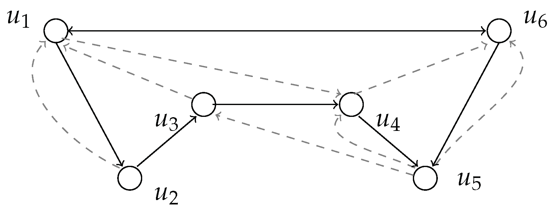
A signed graph is the overlapping of two directed graphs, and , over the same set of nodes. For an example of the definitions to follow, refer to Figure 1.
For any , we denote as and , respectively, the sets of in-friends and of in-enemies of u, that is, the in-neighbors of u in and in :
Similarly, for each , we define the sets of out-friends and out-enemies of u as
A path in between any pair of nodes in V is called a positive path and denotes the maximum length of a shortest positive path. For , we denote as the set of nodes such that, for any , G contains a positive path from v to u and, for , as the length of a shortest positive path in G from v to u. Finally, for and ,
Negative paths, , , and are defined similarly.
Let and be, respectively, a node-weight and an arc-weight function. A set of initially informed nodes (all the remaining nodes in being unaware) may eventually start a -diffusion process: at time step 1 any node becomes informed if the cumulative weight of its in-friends is at least while the cumulative weight of its in-enemies is less than , that is
We denote as the set of nodes becoming informed at time step 1.
Conversely, if the cumulative weight of u’s in-enemies is at least , then the negative influence that u receives from will induce it to remain in the unaware state forever, that is, at any successive time step u will never become informed. We say u becomes refractory. Needless to say, if neither the cumulative weight of u’s in-friends nor the cumulative weight of u’s in-enemies reaches , u does not change its state.
Inductively, if denotes the set of nodes becoming informed at time step j, an unaware node becomes refractory at time step if
while it becomes informed if (1) does not hold and
A set is a target set for if . Needless to say, the size of a target set is .
The Signed Target Set Selection problem (STSS) asks for computing a minimum size target set for a given signed graph with node- and arc-weight functions and w. The Unweighted Signed Target Set Selection problem (USTSS) is the restriction of STSS in which all node- and arc-weights equal 1.
Notice that, if for some , then for all . The latency of a diffusion process is, therefore, defined as the integer such that and . The t-TSS (t-USTSS) problem asks for computing minimum size target sets yielding diffusion processes of latency t.
4. Complexity of Approximation of USTSS and 2-USTSS
We shortly recall that an A-reduction (see [44]) is a reduction between a pair of (NPO) optimization problems transforming (in polynomial time) instances of a problem P to instances of a problem Q so that a solution for an instance of P can be recovered in polynomial time from a solution of the corresponding instance of Q and, for some , a r-approximate solution for is a -approximate solution for . Informally speaking, A-reductions preserve the approximability properties of (NPO) optimization problems. In this section, we shall prove that 2-USTSS and USTSS are both Min Horn Deletion-complete with respect to A-reductions. Such a result will follow by a couple of A-reductions involving the weakly positive-minimum ones problem proved to be Min Horn Deletion-complete with respect to A-reductions in [44].
In more detail, we first A-reduce the weakly positive-minimum ones problem to 2-USTSS in Section 4.1, and this together with the results in [44], and Lemmas 1 and 2, will prove the following theorem.
Theorem 1.
For any , 2-USTSS (and, hence, USTSS) is NP-hard to approximate to within .
Then, in Section 4.2 we A-reduce USTSS to weakly positive-minimum ones in order to get the Min Horn Deletion-completeness of both USTSS and 2-USTSS. In turn, this implies that 2-USTSS and USTSS are in poly-APX.
Let be a set of boolean variables; a set of clauses (i.e., disjunction of literals) on X such that, for each , contains at most one negative variable is said weakly positive. If f is a set of weakly positive clauses, a clause in f will be called positive if all literals it contains are positive variables, and it will be called negative if it contains one negated variable.
An instance of weakly positive-minimum ones is a pair , where is a set of boolean variables and is a weakly positive set of clauses; the weakly positive-minimum ones problem asks for computing a minimum size subset of X to be set to in order to satisfy all clauses in f.
In what follows, with a slight abuse of notation, we shall sometimes write () as a shorthand to mean that () is a literal of clause (so that is considered as a set of literals, instead of their disjunction). We shall say that a variable is positively contained in a clause if , and that is negatively contained in if .
Let be an instance of weakly positive-minimum ones; without loss of generality, in what follows we shall always assume that at least one clause in f is positive (otherwise all clauses in f would be satisfied by setting to no variable in X) and that each clause in f contains at least a couple of variables (one of which positive). Indeed, if some clause in f consists of a single positive variable then such variable has to be necessarily set to in order to satisfy f, and a smaller set of clauses can be derived by removing from f all clauses containing that variable and an optimum solution for f is obtained by adding the variable to an optimum solution for . Similarly, if some clause in f consists of a single negative variable then such variable has to be necessarily set to in order to satisfy f, and a smaller set of clauses can be derived by removing from f all clauses containing that negative variable and an optimum solution for f is an optimum solution for . Hence, f is satisfied by assigning to all the n variables in X, and f is not satisfied by assigning to all the n variables in X.
4.1. weakly positive-minimum ones 2-USTSS
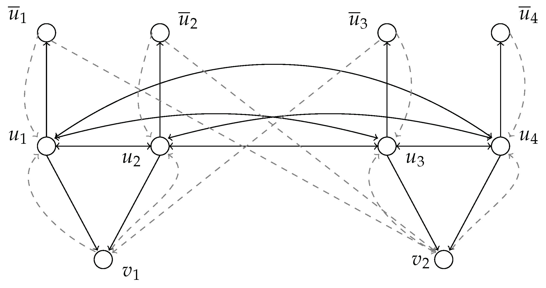
We now derive from an instance of weakly positive-minimum ones a signed network (see Figure 2):
- we set , where , and ;
- for each , is an arc in and is an arc in ;
- for each , is an arc in and is an arc in (that is, nodes in form a clique of positive arcs);
- for each clause and for each positively contained in , is an arc in and is an arc in ;
- if is a negative clause and is its negative variable, then is an arc in ;
- if is a positive clause then, for any , is an arc in .
Needless to say, computing G requires polynomial time in .
The next lemma proves that it suffices to search in for a target set for G.
Lemma 1.
For any target set for G there exists a target set for G such that and .
Proof.
Recall that each clause in f contains at least one positive variable.
Let be a target set for G. Notice that, since all in-friends of any node in are contained in (that is, for any ), then nodes in can get informed by nodes in only; consequently, it must be .
Suppose there exists such that : since , it must be (or could not be informed, contradicting that I is a target set). On the other hand, since and , is able to inform . Finally, since , is unable to inform any node, this proves that is still a target set for G. So, is a target set for G.
Similarly, if there exists , then, since for any positively contained in , is a target set for G only if . On the other hand, since , since , and since , then is able to inform . Since , is unable to inform any other node, and, hence, is still a target set for G, and so is . □
The next lemma shows that the construction defined in this subsection is actually an A-reduction, so completing the proof that weakly positive-min onesUSTSS.
Lemma 2.
For any , with , f is satisfiable by assigning to k variables in X if and only if there exists a target set for G of size k.
Proof.
Suppose f is satisfiable by the truth assignment a assigning to variables in X. We show that the set is a target set for G.
We start by noticing that all nodes in become informed at time step 1, and that all nodes in become informed at time step 1 or 2 so that they cannot negatively influence any node at time step 1. Since a satisfies f, any positive clause contains a (positive) variable such that ; hence, and becomes informed at time step 1. Hence, all nodes in corresponding to positive clauses become informed at time step 1.
Let be a negative clause and let be its negative variable: a satisfies either by assigning to or by assigning both to its negative variable and to at least one of its positive variables. In the former case, becomes informed at time step 2 and, since all nodes corresponding to positive variables in become informed at time step 0 or 1 (whether they are in or not), it cannot forbid to get informed at time step 2. In the latter case, both and become informed at time step 1 so that cannot forbid to get informed.
Hence, all nodes in G are informed (by time step 2), that is, is a target set for G, and .
Conversely, let be a target set for G. By Lemma 1, we can assume .
Let be a positive clause in f. If, for any , then could become informed only at time step 2; since , then there exists so that is informed at time step 1 and, since , it would forbid to become informed, contradicting that is a target set. Hence, for any positive clause in f there exists such that .
Let be a negative clause in f, let be its negative variable and let be its positive variables. If for any , and, hence, , then, as already noticed, could become informed only at time step 2. In this case it must be : indeed, if then would get informed at time step 1 and, since , this would forbid to become informed, so contradicting that is a target set for G. Hence, if for any , then it must be too.
Summarizing, a satisfies each clause in f, that is, a satisfies f, and a assigns to variables. □
We finally observe that the latency of any cascade occurring in the signed graph in the reduction here described is at most 2. This proves that, for any , t-USTSS is min Horn Deletion-hard.
4.2. USTSSweakly positive-minimum ones
We now derive from a signed graph a set of weakly positive clauses.
Before proceeding, we need a preliminary lemma.
Lemma 3.
A set is a target set for if and only if for any
- , and
- for any , it holds that .
Proof.
We start by noticing that, since node thresholds and arc weights are all equal to 1, the diameter of upper bounds the latency of any diffusion process in G: indeed, for any , if any of the u’s neighbors is informed at time step t, either u becomes informed at time step or it will never become informed. As a consequence, for any target set and for any , u may become informed at time step only if .
Suppose is a target set for G; hence, can be partitioned into at most subsets such that all individual-nodes in become informed at time step t, for any . This implies that, for any and for any , and, hence, .
Let , for some : if there exists for some , v would forbid u to get influenced at time step t. Hence, for any , it must hold that , that is, . This proves the first part of the assertion.
Conversely, suppose that, for any , and, for any , it holds that . For any , denote as the set of nodes such that . Since for any node , by hypothesis, all nodes in are influenced at time step 1. Inductively, it can then be proved that, for any , all nodes in , are influenced at time step t. This proves that is a target set for G. □
To model by a weakly positive set of clauses , we start by defining the set of boolean variables, each of which witnesses whether the corresponding node is initially informed or not. Then, we describe the set of clauses defining , which is partitioned into a set P of positive clauses and a set Q of negative clauses: that is, .
Let u be any node and let be the set . P contains a single clause associated to u which models the requirement that u is initially informed or it can become informed in a further step:
Similarly, for any , Q contains a set of clauses associated to u, modeling the requirement that u is initially informed or it can become informed earlier than any node in . For each , contains the clause
and, for each and for each such that , contains the clause
where .
Summarizing, , with and . Needless to say, is computable in polynomial time from G. Furthermore, there is a one-to-one correspondence among subsets of V and truth assignments for X: for any , we denote as the truth assignment corresponding to , that is,
The next lemma proves that the just described construction is actually an A-reduction from USTSS to weakly positive-minimum ones.
Lemma 4.
Let be a signed graph. is a target set for G if and only if the truth assignment satisfies .
Proof.
Let be a target set for G.
For any , since and, for any clause , , then satisfies and every clause in .
For any , since is a target set for G, then, by Lemma 3, : let be such that . By construction, , and, hence, is satisfied by . Furthermore, for any , let be such that : by Lemma 3, for any , and, hence, for any , and for any , is contained in every clause in containing . As a consequence, every clause containing as its negative variable such that , also contains ; since , and, hence, c is satisfied by . This proves that every clause containing as its negative variable such that is satisfied by a.
In conclusion, for any , satisfies and all clauses in .
Conversely, suppose satisfies . For any , since satisfies , there must exist at least one node such that and, hence, . This proves that .
Furthermore, for any and , and for any (that is, and v may become informed by a path from y), any clause in containing has also to contain a positive variable such that . By construction of the clauses in , this implies that , that is, .
By Lemma 3, this proves that is a target set for G. □
5. The 1-USTSS Problem
The 1-USTSS problem is trivially Set Cover-hard: actually, a dominating set of a graph is also a 1-target set for the signed graph where and . Hence, 1-USTSS is non-approximable within for some .
In the remainder of this section, we study the approximability of 1-USTSS.
We start by noticing that if a diffusion process of latency 1 is required to occur, then the A-reduction described in Section 4.2 yields a weakly positive set of clauses such that all its negative clauses have size 2 (that is, they contain exactly one positive literal and one negative literal). In fact, it directly follows from Lemma 3 that is 1-target set for a signed graph if and only if for any
- , and
- for any , it holds that .
As a consequence, for any the set of the negative clauses associated to u (as defined in Section 4.2) is
This proves that the A-reduction shown in Section 4.2 works also as an A-reduction from 1-USTSS to weakly positive minimum ones such that the set of clauses corresponding to a signed graph, besides being weakly positive, has all its negative clauses of size 2. In [44] it is shown that the weakly positive minimum ones problem is B-approximable when restricted to such instances, where B is the maximum size of a positive clause in the set.
The size of the positive clauses in the set described in Section 4.2 is very large: for , , since had to state that u is in or there exists some node in connected to u by a path (of any length). However, when diffusion processes of latency 1 are to be described, can be slightly modified in order to decrease the size of its positive clauses: more precisely, condition a above implies that, for each , where , that is, .
Hence, by denoting as the maximum in-degree of a node in , that is, , the next theorem follows from Lemma 4, from definition (3) and from the already cited result in [44].
Theorem 2.
The 1-USTSS problem is -approximable, where .
We remark that the result in Theorem 2 only depends on the topology of , no matter which is the topology of . Throughout the next subsection we shall follow the opposite way, that is, we shall study the complexity of 1-USTSS in relation to the topology of , no matter which is the topology of .
5.1. 1-USTSS and
Let be a signed graph. Notice that any is a target set for G only if, for each , it holds that . In turn, if I is a target set for G containing u and, hence, , then I must contain also , for any . More precisely, if we define, for each , the set containing u and all the nodes reachable from u by a path in , that is,
then the next fact holds, which follows from the previous observation by a simple inductive argument.
Fact 1: If is a target set for then, for any , .
Observe now that, if is strongly connected, then, for any , it holds that ; hence, by Fact 1, we get
Fact 2: If is strongly connected, then the only target set for G (no matter about its latency) is V.
For any , we define the set
that is, the set of nodes that are or may become informed within time step 1 whenever all nodes in E are contained in the set of the initially informed nodes.
Lemma 5.
is a 1-target set for if and only if and, for any , .
Proof.
If is a 1-target set for , then, trivially, and, by Fact 1, for any , .
Conversely, suppose that and, for any , . Then, for any node ,
- since , there exists such that (that is, y may inform x at time step 1) and, furthermore,
- since for any , , then, for any such that , since and , (that is, any node that could forbid x to become informed is not in I). □
Lemma 5 allows us to prove membership to PO of 1-USTSS when restricted to chain and generalized chain graphs. The chain graph over the node set is made of the set of arcs . A generalized chain graph consists of a set of strongly connected components linked to each other in a chain-like topology, that is, for any and for any , arc exists only if .
Theorem 3.
The 1-USTSS problem restricted to instances such that is a chain or a generalized chain graph is in PO.
Proof.
If is a chain, that is, and , then , and, in general, for , . Hence, .
Correspondingly, : indeed, for any ,
As a consequence, by Lemma 5, is a minimum size 1-target set for G, where .
Let be a generalized chain and let be its strongly connected components. As already stated in the observation leading to Fact 2, for any and for any , it holds that : hence, in what follows we shall use the notation to refer to any set for .
By the same argument holding for chain graphs, for any , we get that contains all nodes in any with . Hence, again by a similar reasoning to that holding in the chain case, since , we get that is a minimum size 1-target set for G, where . □
Lemma 5 shows that any 1-target set is actually obtained by choosing a subcollection of sets in the collection . We now introduce the collection as the closure of under non-empty intersections: that is, , and, for each such that , .
The introduction of allows us to describe any target set for G as the union of pairwise disjoint subsets, that is:
Fact 3: For any target set I for , there exists such that and, for any , .
Based on fact 3, we now show how to get in over polynomial time a -approximate solution for 1-USTSS by a (non-polynomial-time) reduction from 1-USTSS to minimum Weighted Set Cover (WSC) and by the -approximation algorithm for WSC [45]. Later in this section, we shall discuss cases in which the procedure overall runs in polynomial time.
Recall that an instance of WSC is a triple where , , and ; the goal is finding a minimum weight set such that , where the weight of is defined as .
Let be a signed graph; the corresponding instance of WSC is obtained by setting , and, for each , .
Lemma 6.
Let be a signed graph and ; , is a 1-target set for G if and only if is a set cover for . Furthermore, if are pairwise disjoint then .
Proof.
Let be elements of and let . By definition, is a 1-target set for G if and only if . Hence,
that is, is a set cover of X.
If are pairwise disjoint, then
□
The previous lemma shows that the proposed transformation is actually a reduction and that, if a 1-target set for G is described as the union of pairwise disjoint elements of , then its size equals the weight of the corresponding set cover of .
Notice that, if is an optimal solution for the instance of WSC corresponding to G then, for any , it holds that : indeed, if there exist such that , since and, thus, and, moreover, , then the set would still be a set cover for and
so contradicting that is an optimal solution for .
As a consequence of the previous reasoning and of Lemma 6, if is an optimal solution for the instance of WSC corresponding to G then the set is an optimal 1-target set for G.
Consider now the following procedure to compute a 1-target set of a signed graph : first compute set , then the instance of WSC and, finally apply to it Chvatal’s algorithm in [45] to get a solution such that , where is an optimal solution for .
Needless to say, it may well happen that the sets are not pairwise disjoint, so that the second part of Lemma 6 cannot be exploited to bound the size of the so found 1-target set. In this case, we derive from a new set cover for such that and are pairwise disjoint: set and then, while there exist such that , replace in the pair by . Notice that, at any replacement, is still a set cover for and its weight does not increase since
Hence, in -time we have computed a 1-target set for G such that
This proves the following theorem.
Theorem 4.
It is possible to find an -approximate solution for an instance of 1-USTSS in -time.
In general, the algorithm described so far does not run in polynomial time since the size of is not polynomially bounded by . Actually, the size of is strongly related to the topology of and in what follows we shall consider topologies yielding families of polynomial size. Without loss of generality, we shall only consider (weakly) connected graphs.
A source tree is a weakly connected directed graph containing one source node s connected to each other node of the graph by exactly one path and such that, for any pair of nodes u and v, if there is a path from u to v then such a path is contained in the path from s to v. Similarly as for the generalized chains, a generalized source tree consists of a set of strongly connected components linked to each other in a source tree-like topology. This means that, if we replace each strongly connected component in by a single node, we get a source tree.
Corollary 1.
1-USTSS is -approximable for instances such that is a source tree or a generalized source tree.
Proof.
When the graph is a (directed) source tree then, for each , is the set of nodes in the subtree of rooted at u. Hence, if then either or . This proves that , that is, .
A similar reasoning to that used in Theorem 3 for the case of the generalized chain allows to extend to generalized trees the result about trees. □
6. Conclusions and Open Problems
This paper aims at studying the impact of negative relations (witnessing antagonism or distrusting) to diffusion processes within a network. We first defined a diffusion rule, generalizing the Linear Threshold Model to signed relations, and then we studied the complexity of computing a minimum size target set with respect to it. We finally considered a set of restrictions under which the problem is approximable to some extent.
Our approximability results all refer to 1-target sets. We proved that the lower bound on the approximation ratio is tight for a simple topology of the graph of the negative relations, that is, the generalized source tree, and that our problem is in PO if such graph is a generalized chain. Needless to say, broadening the set of topologies of the graph of the negative relations still yielding reasonable approximation is an interesting research direction. After the results in [3,24], studying the problem restricted to graphs of bounded tree-width or clique-width looks like a worthwhile research direction.
After the discussion in Section 2, we remark that 1-target sets correspond to some kind of dominating sets, that we have called dominating sets with constrained pairs: given a graph and a set , any node is dominated by a set if or v has a neighbor in D and, for each , . We have, thus, proved that the bound on the approximation ratio of the Dominating Set problem still holds for our constrained problem when is a generalized source tree. Again, broadening the set of topologies of the graph of the negative relations still yielding -approximation seems an interesting research direction. Finally, our -approximation ratio is exponentially far from the -approximation ratio holding for the minimum Dominating Set problem [43]. Narrowing the gap is an issue deserving attention too.
Author Contributions
Conceptualization, M.D.I. and G.V.; Methodology, M.D.I. and G.V.; Formal analysis, M.D.I. and G.V.; Writing—original draft preparation, M.D.I. and G.V.; Writing—review and editing, M.D.I. and G.V. All authors have read and agreed to the published version of the manuscript.
Funding
This research received no external funding.
Conflicts of Interest
The authors declare no conflict of interest.
References
- Domingos, P.; Richardson, M. Mining the Network Value of Customers. In Proceedings of the Seventh ACM SIGKDD International Conference on Knowledge Discovery and Data Mining, San Francisco, CA, USA, 26 August 2001; pp. 57–66. [Google Scholar]
- Richardson, M.; Domingos, P. Mining Knowledge-sharing Sites for Viral Marketing. In Proceedings of the Eighth ACM SIGKDD International Conference on Knowledge Discovery and Data Mining, Edmonton, AB, Canada, 23 July 2002; pp. 61–70. [Google Scholar]
- Ben-Zwi, O.; Hermelin, D.; Lokshtanov, D.; Newman, I. Treewidth governs the complexity of target set selection. Discret. Optim. 2011, 8, 87–96. [Google Scholar] [CrossRef] [Green Version]
- Chen, W.; Wang, C.; Wang, Y. Scalable Influence Maximization for Prevalent Viral Marketing in Large-scale Social Networks. In Proceedings of the 16th ACM SIGKDD International Conference on Knowledge Discovery and Data Mining, Washington, DC, USA, 25 July 2010; pp. 1029–1038. [Google Scholar]
- Granovetter, M. Threshold Models of Collective Behavior. Am. J. Sociol. 1978, 6, 1420–1443. [Google Scholar] [CrossRef] [Green Version]
- Kempe, D.; Kleinberg, J.; Tardos, É. Maximizing the Spread of Influence Through a Social Network. In Proceedings of the Ninth ACM SIGKDD International Conference on Knowledge Discovery and Data Mining, Washington, DC, USA, 24 August 2003; pp. 137–146. [Google Scholar]
- Kempe, D.; Kleinberg, J.; Tardos, É. Influential Nodes in a Diffusion Model for Social Networks. In Automata, Languages and Programming; Caires, L., Italiano, G.F., Monteiro, L., Palamidessi, C., Yung, M., Eds.; Springer: Berlin, Germany, 2005; Volume 3580, pp. 1127–1138. [Google Scholar]
- Leskovec, J.; Adamic, L.A.; Huberman, B.A. The Dynamics of Viral Marketing. ACM Trans. Web 2007, 1, 5-es. [Google Scholar] [CrossRef] [Green Version]
- Contagion, M.S. The Review of Economic Studies; Oxford University Press: New York, NY, USA, 2000; pp. 57–78. [Google Scholar]
- Ackerman, E.; Ben-Zwi, O.; Wolfovitzv, G. Combinatorial Model and Bounds for Target Set Selection. Theor. Comput. Sci. 2010, 411, 4017–4022. [Google Scholar] [CrossRef] [Green Version]
- Bazgan, C.; Chopin, M.; Nichterlein, A.; Sikora, F. Parameterized approximability of maximizing the spread of influence in networks. J. Discret. Algorithms 2014, 27, 54–65. [Google Scholar] [CrossRef]
- Centeno, C.C.; Dourado, M.C.; Penso, L.D.; Rautenbach, D.; Szwarcfiter, J.L. Irreversible conversion of graphs. Theor. Comput. Sci. 2011, 412, 3693–3700. [Google Scholar] [CrossRef] [Green Version]
- Chen, N. On the approximability of influence in social networks. SIAM J. Discret. Math. 2009, 23, 1400–1415. [Google Scholar] [CrossRef]
- Chiang, C.Y.; Huang, L.H.; Li, B.J.; Wu, J.; Yeh, H.G. Some results on the target set selection problem. J. Comb. Optim. 2013, 25, 702–715. [Google Scholar] [CrossRef] [Green Version]
- Chiang, C.Y.; Huang, L.H.; Yeh, H.G. Target Set Selection Problem for Honeycomb Networks. SIAM J. Discret. Math. 2013, 27, 310–328. [Google Scholar] [CrossRef] [Green Version]
- Chopin, M.; Nichterlein, A.; Niedermeier, R.; Weller, M. Constant Thresholds Can Make Target Set Selection Tractable. Theor. Comput. Syst. 2014, 55, 61–83. [Google Scholar] [CrossRef] [Green Version]
- Zaker, M. On dynamic monopolies of graphs with general thresholds. Discret. Math. 2012, 312, 1136–1143. [Google Scholar] [CrossRef] [Green Version]
- Bettencourt, L.M.A.; Cintron-Arias, A.; Kaiser, D.I.; Castillo-Chavez, C. The power of a good idea: Quantitative modeling of the spread of ideas from epidemiological models. Phys. Stat. Mech. Appl. 2006, 364, 513–536. [Google Scholar] [CrossRef] [Green Version]
- Nekovee, M.; Moreno, Y.; Bianconi, G.; Marsili, M. Theory of rumour spreading in complex social networks. Phys. Stat. Mech. Appl. 2007, 374, 467–470. [Google Scholar] [CrossRef] [Green Version]
- Goldenberg, J.; Libai, B.; Muller, E. Talk of the network: A complex systems look at the underlying process of word-of-mouth. Market. Lett. 2001, 12(3), 211–223. [Google Scholar] [CrossRef]
- Flocchini, P.; Lodi, E.; Luccio, F.; Pagli, L.; Santoro, N. Irreversible dynamos in tori. In Euro-Par’98 Parallel Processing; Pritchard, D., Reeve, J., Eds.; Springer: Berlin, Germany, 1998; Volume 1470, pp. 554–562. [Google Scholar]
- Luccio, F.; Pagli, L.; Sanossian, H. Irreversible dynamos in butterflies. In Proceedings of the 6th Colloquium on Structural Information and Communication Complexity, Lacanau-Ocean, France, 1–3 July 1999; pp. 204–218. [Google Scholar]
- Peleg, D. Size bounds for dynamic monopolies. Discret. Appl. Math. 1998, 86, 263–273. [Google Scholar] [CrossRef] [Green Version]
- Cicalese, F.; Cordasco, G.; Gargano, L.; Milanic̎, M.; Vaccaro, U. Latency-Bounded Target Set Selection in Social Networks. Theor. Comput. Sci. 2014, 535, 1–15. [Google Scholar] [CrossRef]
- Dreyer Jr, P.A.; Roberts, F.S. Irreversible k-threshold processes: Graph-theoretical threshold models of the spread of disease and of opinion. Discret. Appl. Math. 2009, 157, 1615–1627. [Google Scholar] [CrossRef]
- Gargano, L.; Hell, P.; Peters, J.G.; Vaccaro, U. Influence Diffusion in Social Networks under Time Window Constraints. Theor. Comput. Sci. 2015, 584, 53–66. [Google Scholar] [CrossRef]
- Dreyer, P.A. Applications and Variations of Domination in Graphs. Ph.D. Thesis, Rutgers University, Camden, NJ, USA, 2000. [Google Scholar]
- Alba, J.W.; Hutchinson, J.W.; Lynch, J.G. Memory and decision making. In Handbook of Consumer Behavior; Robertson, T.S., Kassarjian, H., Eds.; Prentice-Hall: Englewood Cliffs, NJ, USA, 1991; pp. 1–49. [Google Scholar]
- Chen, Y.; Iver, G.; Pazgal, A. Limited Memory, Categorization and Competition. Market. Sci. 2010, 29, 650–670. [Google Scholar] [CrossRef] [Green Version]
- Chen, W.; Collins, A.; Cummings, R.; Ke, T.; Liu, Z.; Rincon, D.; Sun, X.; Wang, Y.; Wei, W.; Yuan, Y. Influence maximization in social networks when negative opinions may emerge and propagate. In Proceedings of the 2011 SIAM International Conference on Data Mining, Mesa, AZ, USA, 28–30 April 2011; pp. 379–390. [Google Scholar]
- Nazemian, A.; Taghiyareh, F. Influence maximization in independent cascade model with positive and negative word of mouth. In Proceedings of the 6th International Symposium on Telecommunications (IST), Tehran, Iran, 6–8 November 2012; pp. 854–860. [Google Scholar]
- Stich, L.; Golla, G.; Nanopoulos, A. Modelling the spread of negative word-of-mouth in online social networks. J. Decis. Syst. 2014, 23, 203–221. [Google Scholar] [CrossRef]
- Yang, S.; Wang, S.; Truong, V.A. Online Learning and Optimization Under a New Linear-Threshold Model with Negative Influence. arXiv 2019, arXiv:1911.03276. [Google Scholar]
- Ahmed, S.; Ezeife, C.I. Discovering influential nodes from trust network. In Proceedings of the 28th Annual ACM Symposium on Applied Computing, New York, NY, USA, 18 March 2013; pp. 121–128. [Google Scholar]
- Li, Y.; Chen, W.; Wang, Y.; Zhang, Z.L. Influence diffusion dynamics and influence maximization in social networks with friend and foe relationships. In Proceedings of the Sixth ACM International Conference on Web Search and Data Mining, Rome, Italy, 4 February 2013; pp. 657–666. [Google Scholar]
- Easley, D.; Kleinberg, J. Networks, Crowds, and Markets: Reasoning about a Highly Connected World. Significance 2012, 9, 43–44. [Google Scholar]
- Galhotra, S.; Arora, A.; Roy, S. Holistic influence maximization: Combining scalability and efficiency with opinion-aware models. In Proceedings of the 2016 International Conference on Management of Data, San Francisco, CA, USA, 14 June 2016; pp. 743–758. [Google Scholar]
- Hosseini-Pozveh, M.; Zamanifar, K.; Naghsh-Nilchi, A.R.; Dolog, P. Maximizing the spread of positive influence in signed social networks. Intell. Data Anal. 2016, 20, 199–218. [Google Scholar] [CrossRef]
- Baumeister, R.F.; Bratslavsky, E.; Finkenauer, C. Bad is stronger than good. Rev. Gen. Psychol. 2001, 5, 323–370. [Google Scholar] [CrossRef]
- Peeters, G.; Czapinski, J. Positive-negative asymmetry in evaluations: The distinction between affective and informational negativity effects. Eur. Rev. Soc. Psychol. 1990, 1, 33–60. [Google Scholar] [CrossRef]
- Rozin, P.; Royzman, E.B. Negativity bias, negativity dom- inance, and contagion. Personal. Soc. Psychol. Rev. 2001, 5, 296–320. [Google Scholar] [CrossRef]
- Taylor, S.E. Asymmetrical effects of positive and negative events: The mobilization-minimization hypothesis. Psychol. Bull. 1991, 110, 67–85. [Google Scholar] [CrossRef]
- Foerster, K.T. Approximating Fault-Tolerant Domination in General Graphs. In Proceedings of the Tenth Workshop on Analytic Algorithmics and Combinatorics (ANALCO), New Orleans, LA, USA, 6 January 2013. [Google Scholar]
- Khanna, S.; Sudan, M.; Trevisan, L.; Williamson, D.P. The approximability of constraint satisfaction problems. SIAM J. Comput. 2000, 30(6), 1863–1920. [Google Scholar] [CrossRef] [Green Version]
- Chvátal, V. A greedy heuristic for the set covering problem. Math. Oper. Res. 1979, 4, 233–235. [Google Scholar] [CrossRef]
Figure 1.
A signed graph . Arcs in are black, arcs in are dashed. In this example, , , , , and . Again, , , and, by setting , and . Finally, (a maximum length positive shortest path being ) and (a maximum length negative shortest path being ).
Figure 1.
A signed graph . Arcs in are black, arcs in are dashed. In this example, , , , , and . Again, , , and, by setting , and . Finally, (a maximum length positive shortest path being ) and (a maximum length negative shortest path being ).

Figure 2.
Reducing WEAKLYmathsizesmall POSITIVEmathsizesmall MINIMUMmathsizesmall ONESmathsizesmall to USTSS: , with and . Arcs in are dashed.
Figure 2.
Reducing WEAKLYmathsizesmall POSITIVEmathsizesmall MINIMUMmathsizesmall ONESmathsizesmall to USTSS: , with and . Arcs in are dashed.

© 2020 by the authors. Licensee MDPI, Basel, Switzerland. This article is an open access article distributed under the terms and conditions of the Creative Commons Attribution (CC BY) license (http://creativecommons.org/licenses/by/4.0/).
Share and Cite
MDPI and ACS Style
Di Ianni, M.; Varricchio, G. Latency-Bounded Target Set Selection in Signed Networks. Algorithms 2020, 13, 32. https://0-doi-org.brum.beds.ac.uk/10.3390/a13020032
AMA Style
Di Ianni M, Varricchio G. Latency-Bounded Target Set Selection in Signed Networks. Algorithms. 2020; 13(2):32. https://0-doi-org.brum.beds.ac.uk/10.3390/a13020032
Chicago/Turabian StyleDi Ianni, Miriam, and Giovanna Varricchio. 2020. "Latency-Bounded Target Set Selection in Signed Networks" Algorithms 13, no. 2: 32. https://0-doi-org.brum.beds.ac.uk/10.3390/a13020032
Note that from the first issue of 2016, this journal uses article numbers instead of page numbers. See further details here.