Optimization of Constrained Stochastic Linear-Quadratic Control on an Infinite Horizon: A Direct-Comparison Based Approach


1
Department of Automation, Shanghai Jiaotong University, Shanghai 200240, China
2
School of Economics and Management, Fuzhou University, Fuzhou 350108, China
*
Author to whom correspondence should be addressed.
Algorithms 2020, 13(2), 49; https://0-doi-org.brum.beds.ac.uk/10.3390/a13020049
Submission received: 20 January 2020
/
Revised: 15 February 2020
/
Accepted: 19 February 2020
/
Published: 24 February 2020
Abstract
:In this paper we study the optimization of the discrete-time stochastic linear-quadratic (LQ) control problem with conic control constraints on an infinite horizon, considering multiplicative noises. Stochastic control systems can be formulated as Markov Decision Problems (MDPs) with continuous state spaces and therefore we can apply the direct-comparison based optimization approach to solve the problem. We first derive the performance difference formula for the LQ problem by utilizing the state separation property of the system structure. Based on this, we successfully derive the optimality conditions and the stationary optimal feedback control. By introducing the optimization, we establish a general framework for infinite horizon stochastic control problems. The direct-comparison based approach is applicable to both linear and nonlinear systems. Our work provides a new perspective in LQ control problems; based on this approach, learning based algorithms can be developed without identifying all of the system parameters.
1. Introduction
In this paper we study the discrete-time stochastic linear-quadratic (LQ) control optimal problem with conic control constraints and multiplicative noises on an infinite horizon. There exist in the literature various studies on the estimation and control problems of systems with a multiplicative noise [1,2]. As for the LQ type of stochastic optimal control problems with multiplicative noise, investigations have been focused on the LQ formulation with indefinite penalty matrices on control and state variables for both continuous-time and discrete-time models (see, e.g., [3,4]).
In an LQ optimal problem, the system dynamics are both linear in state and control variables, and the cost function is quadratic in these two variables [5]. One important attractive quality of the LQ type of optimal control models is its explicit control policy which can be derived by solving the corresponding Riccati equation. Due to the elegant structure, the LQ problem has always been a hot issue in optimal control research. Since the fundamental research on deterministic LQ problems by Kalman [6], there have been a great number of studies on it; see [5,7,8]. In the past few years, stochastic LQ problems have drawn more and more attention on this topic, due to the promising applications in different fields, including dynamic portfolio management, financial derivative pricing, population models, and nuclear heat transfer problems; see [9,10,11].
This paper is motivated by two recent developments: LQ optimal control and Markov decision problems (MDPs). First, the constrained LQ problem is significant in both theory and applications. Due to the constraints on state and control variables, it is hard to obtain the explicit control policy by solving the Riccati equation [5]. Recently, there have been studies regarding the constrained LQ optimal control problems, such as [12,13,14]. Meanwhile, in real applications, considering some practical limits, such as the risk or the economic regulations, we have to take some constraints on the control variables into the consideration. In the LQ control problems, including the positivity constraint for the control, some literature, [15,16], propose the optimality conditions and some numerical methods to characterize the optimal control policy. In this paper, we characterise the limits as the conic control constraints considering the real applications.
Work by Cao [17] and Puterman [18] demonstrate that stochastic control problems can be viewed as Markov decision problems. Therefore, the constrained stochastic LQ control problem can be formulated as an MDP, such as [19]. A direct-comparison based approach (or relative optimization), which originated in the area of discrete event systems, has been developed in the past years for the optimization of MDPs [17].
With this approach, optimization is based on the comparison of the performance measures of the system under any two policies. It is intuitively clear, and it can provide new insights, leading to new results to many problems, such as [20,21,22,23,24,25,26]. This approach is very convenient and suitable to the performance optimization problems, leading to results including the property of under-selectivity in time-nonhomogeneous Markov processes [24]. In this paper, we show that the special features of the constrained stochastic LQ optimal control make it possible to be solved by the direct-comparison based approach, leading to some new insights for the problem.
In our work, we consider the stochastic LQ control problem through an MDP formulation in the infinite horizon. Through the direct-comparison based approach [17], we first derive the performance potentials for the LQ problem by utilizing the state separation property of the system structure. Based on this, we successfully derive the optimality conditions and the stationary optimal feedback control. We show that the optimal control policy is a piece-wise affine function with respect to the state variables. In real applications, the proposed methodology can be used in many fields, such as system risk contagion [26] and power grid systems [27].
Our work provides a new perspective for LQ control problems. Compared with the former literature, such as [5,13], we still consider the multiplicative noises. We establish a general framework for studying infinite horizon stochastic control problems. With the direct-comparison based approach, which is applicable to both linear and nonlinear systems, we propose more results for the performance optimization problems, and the results can be extended easily. In addition, without identifying all the system parameters, this approach can be implemented on-line, and learning based algorithms can be developed.
The paper is organized as follows. Section 2 introduces an MDP formulation of the constrained stochastic LQ problem with multiplicative noises; some preliminary knowledge on MDP and the state separation property is also provided. In Section 3, we derive the performance difference formula, which is the foundation of the performance optimization; based on it, the Poisson equation and Dynkin’s formula can be obtained. Then we derive the optimality condition and the optimal policy through the performance difference formula. In Section 4, we illustrate the results by numerical examples. Finally, we conclude the paper in Section 5.
2. Problem Formulation
2.1. Problem with Infinite Time Horizon
In this section, we study the infinite horizon discrete-time stochastic LQ optimal control problem, in which the conic control constraints are also considered; see [5,14]. For simplicity of the parameters, we consider a one dimensional dynamic system with a multiplicative noise described by
for time . By denoting as the set of real (nonnegative real) numbers, in this system, and are deterministic values; is the state with being given; and is a feedback control law at time l. For each l, denotes an independent identically distributed one-dimensional multiplicative noise, satisfying a normal distribution with mean 0 and variance . For each l, denotes a one-dimensional noise. and are independent for every .
Now, we consider the conic control constraint sets (cf. [5])
for , where is a deterministic matrix; and is the filtration of the information available at time l. Let be a given closed cone; i.e., whenever and ; and whenever .
The goal of optimization is to minimize the total reward performance measure in a quadratic form:
where and are deterministic. Here we denote the transpose operation by a prime in the superscript, such as . denotes the control sequence . We also assume that (3) exists.
Therefore, the performance function of (3) is
In this paper, we will show that the direct-comparison based approach leads to more new results for the total rewards problem [7], and that the results can be easily extended.
2.2. MDPs with Continuous State Spaces
For a stationary control law , at time , the constraint (2) can be written as
Then the above stochastic control problem can be viewed as an MDP with continuous state spaces. More precisely, plays a similar role of actions in MDPs, and then the control law is the same as a policy.
Consider a discrete-time Markov chain with a continuous state space on . The transition probability can be described by a transition operatorP as
where is the transition probability function, with ; and is any measurable function on . As is independent Gaussian noises, given the current state , under the stationary control satisfies a normal distribution with mean and variance . Then we have the transition function of this system as follows,
Let be the -field of containing all the (Lebesgue) measurable sets. For any set , we can define the identity transition function . if ; otherwise. For any function h and , we have .
The product of two transition functions and is defined as a transition function :
where .
For any transition function P, we can define the kth power, , as , and . Suppose that the Markov chain is time-homogeneous with transition function . Then the k-step transition probability functions, denoted as , are given by the 1-step transition function defined as and
For any function , we have
That is, as an operator, we have . Recursively, we can prove that .
Suppose that a Markov chain with a continuous state space on has a steady-state distribution satisfying . Define function for all . We denote the performance potential g as a function which satisfies the Poisson equation (cf. [17])
where I and P are two transition functions, and . Then if g is a solution to (7), so is , with any constant c. We define
and assume the limit exists for . Then we have the following lemma,
2.3. State Separation Property
In order to derive the explicit solution of the stochastic LQ control problem with conic constraints, Reference [14] gives the following lemma for the state separation property of the LQ problem,
Lemma 2
(State Separation [14]). In the system (1), for any , the optimal solution for problem (3) at time l is a piecewise linear feedback policy
for , where associated with the control constraint sets ; , are the optimal values of two correspondent auxiliary optimization problems, and the superscript “*” corresponds to the optimal control.
Based on (10) in Lemma 2, the stationary control can be written as , where is an indicator function, such that , if the condition B holds true and otherwise; and . Applying this control, the system dynamics (1) becomes
for , where
Moreover, the performance measure (3) becomes
where and . Therefore, the performance function (4) becomes
It is easy to verify that and are positive semi-definite. We assume that this one-dimensional state system is stable, and then the spectral radiuses of and are less than 1, i.e., . In the next section, we will derive the performance potentials for the LQ problem, which is the foundation of the performance optimization. Based on this, the Poisson equation and the Dynkin’s formula can be derived. The direct-comparison based approach provides a new perspective for this problem, and the results can be extended easily.
3. Performance Optimization
In this section, utilizing the state separation property, we derive the performance difference formula, which compares the performance measures of any tow policies, and then derive the optimality condition and the optimal policy with the direct-comparison based approach.
3.1. Performance Difference Formula
We denote and . Then we have the performance function as . With the initial condition , by (5), (6), (11), and (13), the performance operator is
where
and
with as the probability density function of a standard normal distribution. We can verify that and are both nonnegative constants, with .
As , continuing this process, we obtain
where
We set
In order to ensure the stability of the system, Reference [14] gives some assumptions. Here we assume . Then we have
Therefore, we have
We denote and . Based on the above claims, we obtain that and would converge when . Thus we denote
Based on the definition of total rewards (3), we have
Then we have proved that the closed-loop system (11) is -asymptotically stable, i.e., Therefore, the total rewards exists, that is, a piecewise quadratic function with positive semi-definite matrices and .
Now, we define the discrete version of generator, for any function , such that
By (5) and (20), we obtain the discrete version of Dynkin’s formula as
and if the limit exists, then
Now, we consider two policies , resulting in two independent Markov chains and in the same state space , with , and , respectively. Let . Applying the Dynkin’s Formula (22) on with yields
Noting that , and due to asymptotical stability. Then by (23), we obtain the performance difference formula:
3.2. Optimal Policy
Based on the performance difference Formula (24), we have the following optimality condition.
Theorem 1
(Optimality Condition). A policy in is optimal if, and only if,
From (25), the optimality equation is:
Proof.
First, the “if” part follows from the performance difference Formula (24) and the Poisson Equation (21).
Next, we prove the “only if” part: Let be an optimal policy. We need to prove that (25) holds. Suppose that this is not true. Then, there must exist one policy, denoted as , such that (25) does not hold. That is, there must be at least one state, denoted as y, such that
Then we can create a policy by setting when , and when . We have . This contradicts to the fact that is an optimal policy. □
Based on the optimality condition, the optimal control can be obtained by developing policy iteration algorithms. Roughly speaking, we start with any policy . At the kth step, , given a piecewise linear policy , where , we want to find a better policy by (26). We consider any policy . Setting , by , , and , we have
where and satisfy Equations (15) and (16), respectively.
It can be seen that if the policy is a piecewise linear control, then we can find an improved policy , which is also piecewise linear. Moreover, if and , i.e., , then the iteration stops. The policy satisfies the optimal condition (26) in Theorem 1, and therefore is an optimal control.
Therefore, we can obtain the optimal policy as follows,
where
Moreover,
The original problem (3) is transformed to two auxiliary optimization problems (29) and (30). Under the optimal control in (28), the closed-loop system (11) is -asymptotically stable. From (19), with the initial condition , we know the optimal total reward performance is
where and satisfy (31) and (32), respectively.
Policy iteration can also be implemented on-line, the performance (potential) can be learned on a sample path without knowing all the transition probabilities. In on-line algorithms, the computation of policy evaluation is , where n is the length of a sample path. Additionally, Reference [14] also provides some algorithms for calculating the optimal policy.
4. Simulation Examples
In this section, we use two numerical examples to illustrate the optimal policy for the constrained LQ control problem (3).
Example 1.
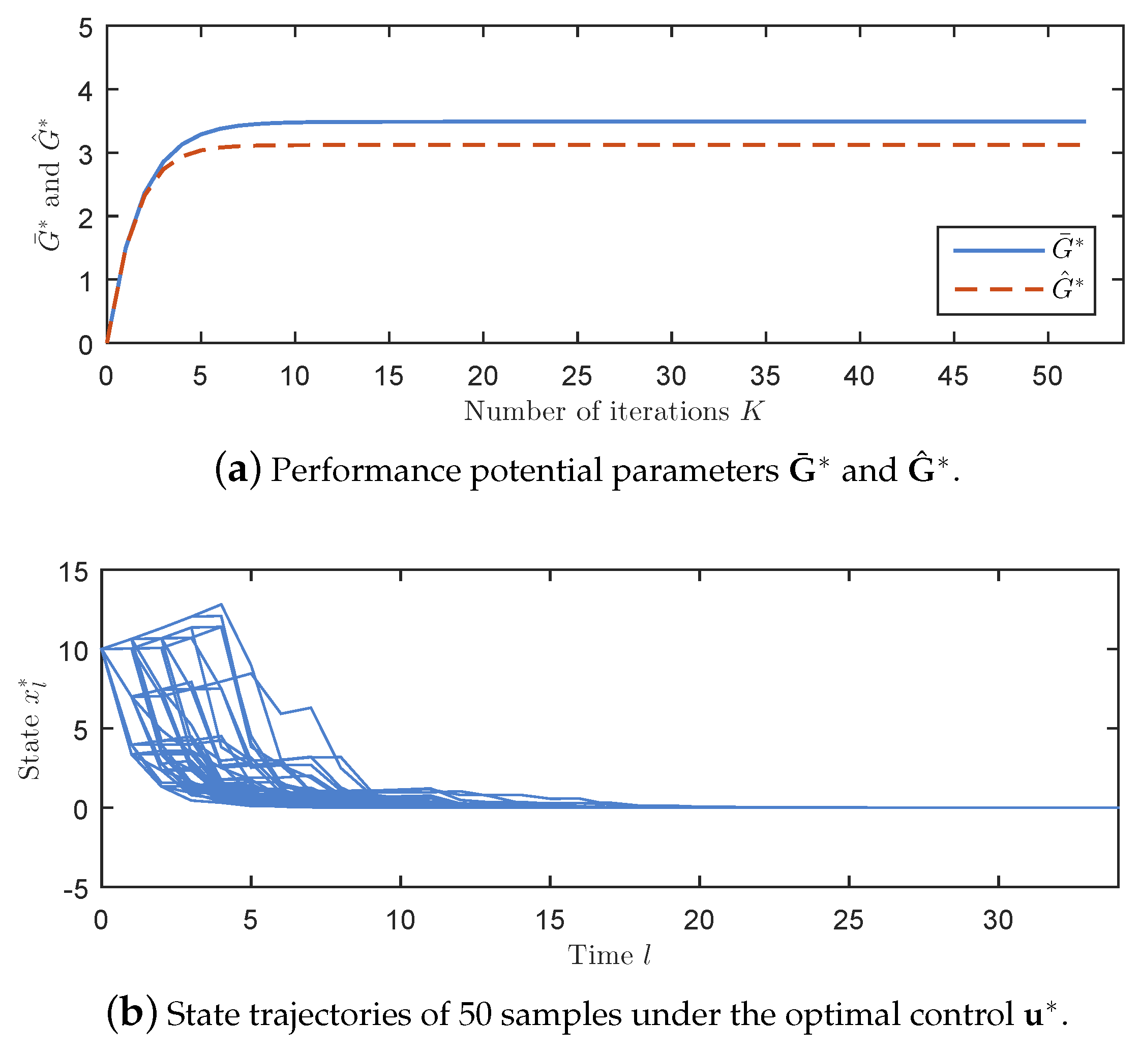
We consider a stochastic LQ system with , , , and . The cost matrix is
For time , the variance of the 0-mean i.i.d. Gaussian noise is . We consider the conic constraint . By applying Theorem 1, the stationary optimal control is , for , where and . Furthermore, the optimal reward performance is .
As shown in Figure 1a plots the outputs and with respect to iteration time K; Figure 1b plots the state trajectories of 50 samples by setting and implementing the stationary optimal control . It can be observed that converges to 0 after time and this closed loop system is asymptotically stable.
Example 2.
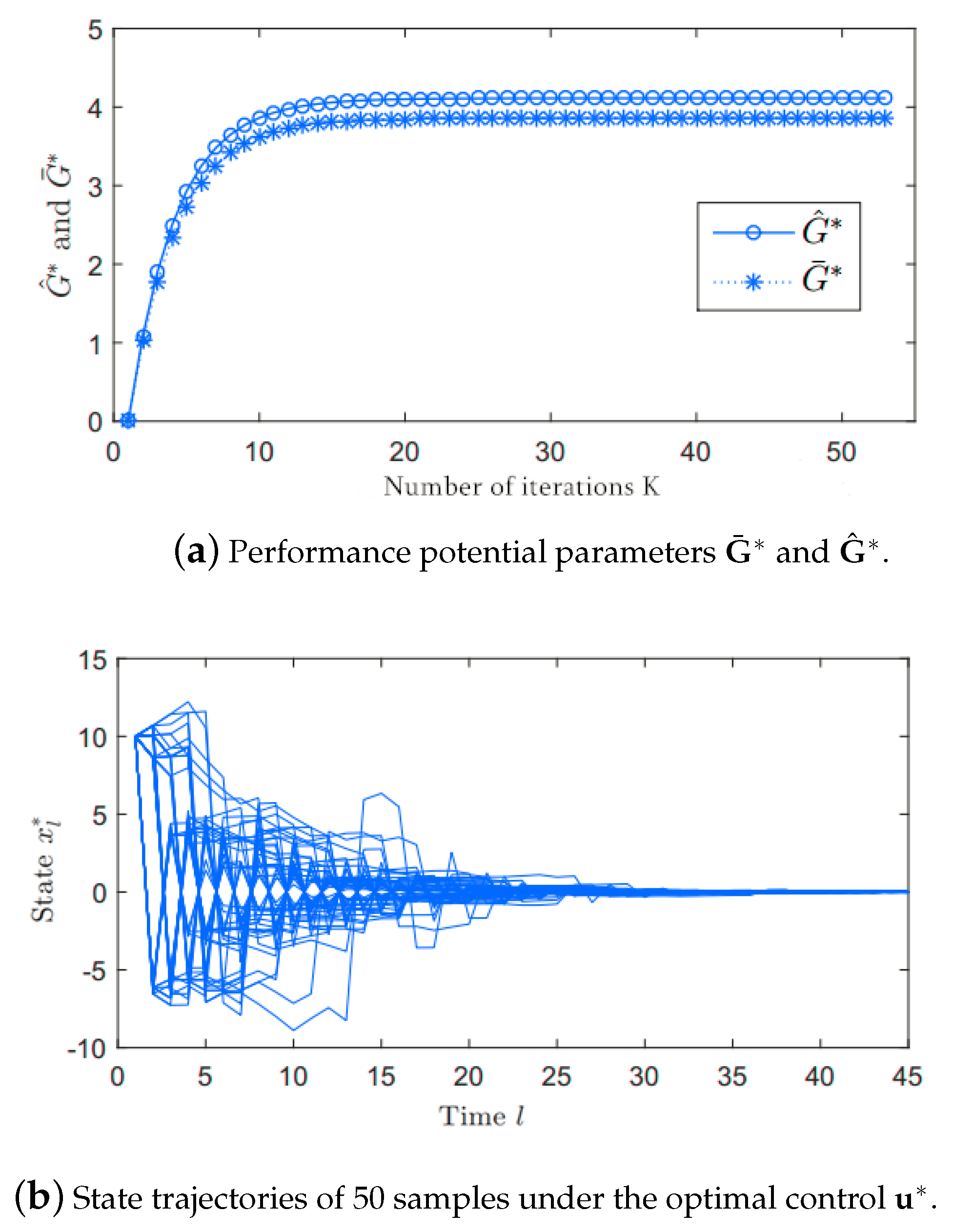
In the second case, we assume and B, following the identical discrete distribution with five cases. We assume , and
each of which has the same probability 0.2. The cost matrix is
For time , the variance of the 0-mean i.i.d. Gaussian noise is . We consider the conic constraint . By applying Theorem 1, the stationary optimal control is , for , where and are identified as follows, and . Furthermore, the optimal reward performance is .
5. Conclusions
In this paper, we apply the direct-comparison based optimization approach to study the rewards optimization of the discrete-time stochastic linear-quadratic control problem with conic constraints on an infinite horizon. We derive the performance difference formula by utilizing the state separation property of the system structure. Based on this, the optimality condition and the stationary optimal feedback control can be obtained. The direct-comparison based approach is applicable to both linear and nonlinear systems. By introducing the the LQ optimization problem, we establish a general framework for studying infinite horizon control problems with total rewards. We verify that the proposed optimal approach can solve the LQ problems. Then we illustrate our results by two simulation examples.
The results can easily be extended to the cases of non-Gaussian noises and average rewards. Most significantly, our methodology can deal with a very general class of linear constraints on state and control variables, which includes the cone constraints, positivity and negativity constraints, and the state-dependent upper and lower bound constraints as a special case. In addition to the problem with the infinite control horizon, our results still fit problems with a finite horizon. In addition, without identifying all the system structure parameters, this approach can also be implemented on-line, and learning based algorithms can be developed.
Finally, this work focuses on the discrete-time stochastic LQ control problem. Our next step is to investigate continuous cases. As the constrained LQ problem has a wide range of applications, we hope to apply our approach in more areas, such as dynamic portfolio management, security optimization of cyber-physical systems, and financial derivative pricing, in our future research.
Author Contributions
Conceptualization, R.X. and X.Y.; methodology, R.X.; validation, R.X., X.Y. and W.W.; formal analysis, X.Y.; data curation, X.Y.; writing–original draft preparation, R.X. and X.Y.; writing–review and editing, R.X., X.Y. and W.W.; supervision, W.W. All authors have read and agreed to the published version of the manuscript.
Funding
This work was supported by the National Natural Science Foundation of China under Grant 61573244 “Stochastic control optimization of uncertain systems based on offset with multiplicative noises and its applications in the financial optimization” and 61521063 “Control theory and techniques: design, control and optimization of network systems”.
Conflicts of Interest
The authors declare no conflict of interest.
Abbreviations
The following abbreviations are used in this manuscript:
| MDP | Markov Decision Process |
| LQ | Linear-Quadratic |
References
- Basin, M.; Perez, J.; Skliar, M. Opitmal filtering for polynomial system wtates with polynomial multiplicative noise. Int. J. Robust Nonlinear Control 2006, 16, 303–314. [Google Scholar] [CrossRef]
- Gershon, E.; Shaked, U. Static H2 and Houtput-feedback of discrete-time LTI systems with state multiplicative noise. Syst. Control Lett. 2006, 55, 232–239. [Google Scholar] [CrossRef]
- Lim, A.B.E.; Zhou, X.Y. Stochastic optimal control LQR control with integral quadratic constraints and indefinite control weights. IEEE Trans. Autom. Control 1999, 44, 1359–1369. [Google Scholar] [CrossRef] [Green Version]
- Zhu, J. On stochastic riccati equations for the stochastic LQR problem. Syst. Control Lett. 2005, 44, 119–124. [Google Scholar] [CrossRef]
- Hu, Y.; Zhou, X.Y. Constrained stochastic LQ control with random coefficients, and application to portfolio selection. SIAM J. Control Optim. 2005, 44, 444–446. [Google Scholar] [CrossRef]
- Kalman, R.E. Contributions to the theory of optimal control. Bol. Soc. Mat. Mex. 1960, 5, 102–119. [Google Scholar]
- Anderson, B.D.; Moore, J.B. Optimal Control: Linear Quadratic Methods; Courier Corporation: North Chelmsford, MA, USA, 2007; pp. 167–189. [Google Scholar]
- Yong, J. Linear-quadratic optimal control problems for mean-field stochastic differential equations. SIAM J. Control Optim. 2013, 51, 2809–2838. [Google Scholar] [CrossRef]
- Gao, J.J.; Li, D.; Cui, X.Y.; Wang, S.Y. Time cardinality constrained mean-variance dynamic portfolio selection and market timing: A stochastic control approach. Automatica 2015, 54, 91–99. [Google Scholar] [CrossRef]
- Costa, O.L.V.; Fragoso, M.D.; Margues, R.P. Discrete-Time Markov Jump Linear Systems; Springer: Berlin, Germany, 2007; pp. 291–317. [Google Scholar]
- Primbs, J.A.; Sung, C.H. Stochastic receding horizon control of contrained linear systems with state and control multiplicative noise. IEEE Trans. Autom. Control 2009, 54, 221–230. [Google Scholar] [CrossRef]
- Dong, Y.C. Constrained LQ problem with a random jump and application to portfolio selection. Chin. Ann. Math. 2019, 39, 829–848. [Google Scholar] [CrossRef] [Green Version]
- Gao, J.J.; Li, D. Cardinality constrained linear quadratic optimal control. IEEE Trans. Autom. Control 2011, 56, 1936–1941. [Google Scholar] [CrossRef]
- Wu, W.P.; Gao, J.J.; Li, D.; Shi, Y. Explicit solution for constrained stochastic linear-quadratic control with multiplicative noise. IEEE Trans. Autom. Control 2019, 64, 1999–2012. [Google Scholar] [CrossRef]
- Campbell, S.L. On positive controllers and linear quadratic optimal control problems. Int. J. Control 1982, 36, 885–888. [Google Scholar] [CrossRef]
- Heemels, W.P.; Eijndhoven, S.V.; Stoorvogel, A.A. Linear quadratic regulator problem with positive controls. Int. J. Control 1998, 70, 551–578. [Google Scholar] [CrossRef]
- Cao, X.R. Stochastic Learning and Optimization: A Sensitivity-Based Approach; Springer: New York, NY, USA, 2007. [Google Scholar]
- Puterman, M.L. Markov Decision Processes: Discrete Stochastic Dynamic Programming; Wiley: New York, NY, USA, 1994. [Google Scholar]
- Chen, R.C. Constrained stochastic control with probabilistic criteria and search optimization. In Proceedings of the 43rd IEEE Conference on Decision and Control (CDC), Nassau, Bahamas, 14–17 December 2004. [Google Scholar]
- Zhang, K.J.; Xu, Y.K.; Chen, X.; Cao, X.R. Policy iteration based feedback control. Automatica 2008, 44, 1055–1061. [Google Scholar] [CrossRef]
- Cao, X.R. Stochastic feedback control with one-dimensional degenerate diffusions and nonsmooth value functions. IEEE Trans. Autom. Control 2018, 62, 6136–6151. [Google Scholar] [CrossRef]
- Cao, X.R.; Wan, X.W. Sensitivity analysis of nonlinear behavior with distorted probability. Math. Financ. 2017, 27, 115–150. [Google Scholar] [CrossRef] [Green Version]
- Xia, L. Mean-variance optimization of discrete time discounted Markov decision processes. Automatica 2018, 88, 76–82. [Google Scholar] [CrossRef] [Green Version]
- Cao, X.R. Optimality consitions for long-run average rewards with underselectivity and nonsmooth features. IEEE Trans. Autom. Control 2017, 62, 4318–4332. [Google Scholar] [CrossRef]
- Xue, R.B.; Ye, X.S.; Cao, X.R. Optimization of stock trading with additional information by Limit Order Book. Automatica 2019. submitted. [Google Scholar]
- Ye, X.S.; Xue, R.B.; Gao, J.J.; Cao, X.R. Optimization in curbing risk contagion among financial institutes. Automatica 2018, 94, 214–220. [Google Scholar] [CrossRef]
- Jia, Q.S.; Yang, Y.; Xia, L.; Guan, X.H. A tutorial on event-based optimization with application in energy Internet. J. Control Theory Appl. 2018, 35, 32–40. [Google Scholar]
Figure 1.
The simulation results of Example 1.

Figure 2.
Simulation Results of Example 2.

© 2020 by the authors. Licensee MDPI, Basel, Switzerland. This article is an open access article distributed under the terms and conditions of the Creative Commons Attribution (CC BY) license (http://creativecommons.org/licenses/by/4.0/).
Share and Cite
MDPI and ACS Style
Xue, R.; Ye, X.; Wu, W. Optimization of Constrained Stochastic Linear-Quadratic Control on an Infinite Horizon: A Direct-Comparison Based Approach. Algorithms 2020, 13, 49. https://0-doi-org.brum.beds.ac.uk/10.3390/a13020049
AMA Style
Xue R, Ye X, Wu W. Optimization of Constrained Stochastic Linear-Quadratic Control on an Infinite Horizon: A Direct-Comparison Based Approach. Algorithms. 2020; 13(2):49. https://0-doi-org.brum.beds.ac.uk/10.3390/a13020049
Chicago/Turabian StyleXue, Ruobing, Xiangshen Ye, and Weiping Wu. 2020. "Optimization of Constrained Stochastic Linear-Quadratic Control on an Infinite Horizon: A Direct-Comparison Based Approach" Algorithms 13, no. 2: 49. https://0-doi-org.brum.beds.ac.uk/10.3390/a13020049
Note that from the first issue of 2016, this journal uses article numbers instead of page numbers. See further details here.