Observability of Uncertain Nonlinear Systems Using Interval Analysis

Abstract

In the field of control engineering, observability of uncertain nonlinear systems is often neglected and not examined. This is due to the complex analytical calculations required for the verification. Therefore, the aim of this work is to provide an algorithm which numerically analyzes the observability of nonlinear systems described by finite-dimensional, continuous-time sets of ordinary differential equations. The algorithm is based on definitions for distinguishability and local observability using a rank check from which conditions are deduced. The only requirements are the uncertain model equations of the system. Further, the methodology verifies observability of nonlinear systems on a given state space. In case that the state space is not fully observable, the algorithm provides the observable set of states. In addition, the results obtained by the algorithm allows insight into why the remaining states cannot be distinguished.

1. Introduction

The constant development in technology offers new possibilities as well as many new challenges. Thus, existing processes are further optimized and new fields of applications are opened up. These topics concern control engineering as well as various other engineering disciplines. In this context, a model-based method is a promising option. Nonlinear, continuous-time models in particular allow accurate and generally valid description of these processes. Since an exact physical modeling of the system is not possible, the model errors are represented by uncertainties.

Assume a nonlinear autonomous system can be described by the set of ordinary differential equations (ODE)

$$\begin{array}{cc}\hfill \dot{x}& =f(x\left(t\right),\alpha ),x\left(0\right)=x_0\hfill \end{array}$$

(1)

and the output

$$\begin{array}{cc}\hfill y& =h\left(x\right(t),\beta )\hfill \end{array}$$

(2)

with $f:{\mathbb{R}}^n\to {\mathbb{R}}^n$ and $h:{\mathbb{R}}^n\to {\mathbb{R}}^p$ as real-analytic functions for $x\left(t\right)\in D_x\subseteq {\mathbb{R}}^n$. The system uncertainties $\alpha \in {\mathbb{R}}^a$ and the uncertainties $\beta \in {\mathbb{R}}^b$ with $a,b\in {\mathbb{N}}_0$ of the measurement are summarized in the uncertainties vector

$$\delta =\{\alpha ,\beta \},$$

(3)

in the case of ${\mathbb{R}}^0$ the corresponding uncertainty is not existent. These $\alpha$ and $\beta$ are interval uncertainties, thus $\alpha \in \left[\underline{\alpha }\overline{\alpha }\right]$ and $\beta \in \left[\underline{\beta }\overline{\beta }\right]$.

To use state feedback controllers, there must be full access to the state vector. To get this access, observers are required for the implementation of these controllers. These observers estimate the non-measurable states on the basis of the available information and provide them to a controller. Before an observer can be developed, it is necessary to verify the observability of the system. In the general case of nonlinear systems, however, this is not a binary decision. It is also possible that a subset $\mathcal{B}\subset D_x\subseteq {\mathbb{R}}^n$ of the states is indistinguishable. Consequently, a nonlinear system can be observable in some areas and not observable in others. Furthermore, the observability of nonlinear systems can be classified into different categorizes such as global, local, weakly observable and others, see [1] for further information. Checking observability of nonlinear systems is an already well-researched domain, yet, had a limited applicability. Nonlinear systems, however, are not inhibited by any limitations that constrain linear systems regarding the precise description of the system dynamics. Nevertheless, the determination whether nonlinear systems are observable has always been a challenging task. In [2] for example, a nonlinear disturbance observer (DOB) is presented. The DOB is used to estimate the disturbances by only utilizing the measurements of the output. The internal uncertainties, external disturbances, parameter uncertainties as well as the modeled dynamics are brought together as a single disturbed term and estimated by the DOB. In order to determine whether this is possible, the nonlinear system needs to be observable.

In the case of nonlinear systems [3,4] (based on [1]) already introduced a possibility to prove local observability using Lie algebra. The set of control Lie algebra consisting of the vector field at position $x\left(t\right)$ is examined. If a subset can be found whose elements multiplied by the Lie derivatives result in zero, then this subset is termed by the authors as unobservability Lie algebra. If the dimension of this subset equals N, a sufficient condition for local observability at point $x\left(t\right)$ can be stemmed. That is, if the subset is equal to the isotropic algebra of the original set. The work of Tibken [5] investigates further how algebraic methods can be used to demonstrate global observability. Therein, systems with polynomial functions are considered. All states that are not distinguishable from the vector $x\left(t\right)$ are considered a ring. The variety of the ideal of this ring is used to prove the global observability of polynomial systems. The investigation of Kawano and Ohtsuka [6] also deals with the observability of polynomial systems. The main difference is that Kawano and Ohtsuka extend the method for non-autonomous systems and find a more general condition.

Another example can be found in [7]. The authors examine the effect on observability if the initial conditions $x\left(0\right)=x_0$ have a probability distribution. This is called ensemble observability problem [8]. The approach here is to determine the trajectories of the initial distribution to reconstruct the probability distribution of the initial states $x_0$. Other works merely reconstruct the associated trajectories.

In order to prove observability, the observability function must be injective. An algorithm for determining the injectivity of a function is described in [9,10]. The method is based on interval arithmetics and determines the injectivity by examining whether the intervals intersect in the mapping for a given interval. This is done iteratively until the width of the intervals is smaller than the width of a comparison interval due to bisection, the hull of all intervals is formed. Afterwards, the resulting hull of intervals is substituted into the Jacobian and the rank determined. The investigated matrix is the interval Jacobian multiplied by the pseudo-inverse midpoint matrix to obtain a square matrix if the interval Jacobian has the dimension $(n\times p)$ with $n\le p$. The suggested methods to check the rank are to test whether the matrix is strictly diagonal dominant or to identify the rank by using the determinant. However, both methods lead to high overestimation. Therefore, it is necessary to bisect often to obtain very small intervals in order to be able to prove the injectivity. Furthermore, the provided and presented solver ITVIA only allows determining the injectivity of functions mapping $\mathbb{R}\to {\mathbb{R}}^2$ or ${\mathbb{R}}^2\to {\mathbb{R}}^2$ [10]. Thereby, the verification of injectivity is impracticable, especially since the number of required Lie derivatives is unknown and cannot be easily varied.

In [11], Röbenack and Reinschke analyze the observability of nonlinear systems. The authors use automatic differentiation to determine the Taylor coefficients of Lie derivatives. The resulting observability matrix is checked on full rank by singular value decomposition. The smallest singular value over time gives the authors information about whether a nonlinear system is observable. The method is capable of determining whether a nonlinear system might be observable. However, it is not able to identify the observable states or which areas are not distinguishable.

In [12] interval arithmetic routines are used to verify the controllability and observability of the states in case of uncertain dynamic systems. For this purpose the observability matrix is constructed using automatic differentiation and the rank is checked. Therefore, the observability can only be verified locally. However, the importance of taking the reachability and observability of states into account for choosing the structures for control laws and state observers in the earliest design stages are shown.

A different approach to prove local as well as global observability of nonlinear systems is presented in [13]. The method considers polynomial systems with a one-dimensional output equation ${\mathbb{R}}^n\to \mathbb{R}$. The authors Röbenack and Voßwinkel use the method of quantor elimination [14] to determine the injectivity of the observability matrix or the observability function, respectively. Depending on the number of Lie derivatives, a binary decision about observability of the system is possible. If the system states are defined as free variables, thus they are not bound to a quantor, it is also possible to specify the restrictions if the algorithm returns false as a result. Thereby, constraints can be specified for which the states are distinguishable. However, this does not allow the exact assignment about which state is indistinguishable from which other state. The advantage of the method presented in [13] is that the nonlinear state space representation can be parameter-dependent. The parameters are also considered as free variables. Therefore, constraints can be found for which the observability of the nonlinear system can be proven.

All of these methods do not provide the determination of indistinguishable states. However, this information may be of particular interest. It would be usable to design a controller such that the system is stabilized while its states remain in the observable domain.

Motivated by these issues, the aim of this work is to contribute a method to analyze the observability of nonlinear systems. The determination of indistinguishable states is provided by the work [15]. This approach is enhanced by system uncertainties in [16], which will be presented in the following. Therefore, this work provides an iterative algorithm based on interval arithmetics to determine whether the nonlinear system (1), (2) is observable. In case that the system is not globally observable, the subset for which observability has been proven is given even if the subset is of a complex structure. Additionally, the information about the indistinguishable states is provided. This is uniquely for this method and allows insight on how to modify an output function to achieve global observability of a nonlinear system. Thus, a method is available, which allows the user to check the observability of a nonlinear system with system uncertainties, whereby only the knowledge of the system equation is required.

The work is structured as follows. In the next section the underlinings idea is presented after a short introduction to the interval arithmetics. Thereafter, the algorithm is explained. In the third section the results of this method are presented followed a discussion in the final section.

2. Materials and Methods

In this section, we will introduce the required math, the method and the proposed algorithm. For convenience, the uncertainties are not considered in the first part of the section. In the algorithm, the handling of uncertainties is resumed. Uncertainties are considered by enclosing them within intervals. These are taken into account by using interval arithmetic in the system equations as parameters and do not need to be considered separately. Beside the inclusion of uncertainties, interval arithmetic ([17,18]) is used to prove observability.

2.1. Interval Arithmetics

Since this journal deals with interval arithmetics (IA), the used denotations will be presented in the following: An interval is defined as

$$\begin{array}{c}\hfill x^I=\left[\underline{x}\overline{x}\right]\end{array}$$

with $\underline{x}\le \overline{x}$. The interval midpoint is defined as

$$\begin{array}{c}\hfill \mathrm{mid}\left(x^I\right)=\frac{\underline{x}+\overline{x}}{2}\end{array}$$

and the radius of the interval as

$$\begin{array}{c}\hfill \mathrm{rad}\left(x^I\right)=\frac{\overline{x}-\underline{x}}{2}.\end{array}$$

(4)

The evaluation of a function f on the interval $x^I$ leads to an interval of the mapping function $f^I=f\left(x^I\right)$. The necessary arithmetic rules are explained in detail in [17]. Unfortunately, dealing with IA leads to an overestimation of $f^I$, unless the variable occurs just once in the function. A simple example is the function $f\left(x\right)=x-x$. The solution of this function is always zero. However, applying IA to this function results in an overestimation of the actual solution. This follows from the arithmetic rules [17] of IA. Overestimation in IA means $f^I$ not only contains solutions which are part of the initial function of this particular $x^I$ but also solutions that emerge due to the arithmetic rules of IA itself. One way of reducing this overestimation is to bisect the interval $x^I=x_a^I\cup x_b^I$ and to use the bisected intervals to evaluate the function. This is state from the fundamental theorem of IA

$$\left\{y|y=f\left(x\right),x\in x^I\right\}\subseteq f\left(x_a^I\right)\cup f\left(x_b^I\right)\subseteq f\left(x^I\right)=:f^I.$$

2.2. Observability of Uncertain Nonlinear Systems

In order to determine the observability of a nonlinear system (1) with the corresponding output function (2), first a definition of global observability is needed. In our case we use the distinguishability to determine wherever the mapping of the trajectories of states can be distinguished.

Definition 1

(Distinguishability). Assume $T>0$. Two states $z^1,z^2\in D_x$ are called indistinguishable on the interval $[0,T]$, if their output courses are identical, that is

$$\begin{array}{c}\hfill \forall t\in [0,T]:h\left(\phi \left(t,z^1\right)\right)=h\left(\phi \left(t,z^2\right)\right).\end{array}$$

(5)

Otherwise, the states are called distinguishable [1,19].

Thereby, the flux $\phi (t,x)$ of the vector field f on the output function h can be formulated as the convergent Taylor series

$$\begin{array}{c}\hfill y\left(t\right)=h\left(\phi \left(t,x\right)\right)={\displaystyle \sum _{k=0}^{\infty }}\frac{t^k}{k!}{L}_f^{k}h\left(x\right).\end{array}$$

(6)

Definition 1 is used to check wherever two states are indistinguishable. To obtain a statement about the entire nonlinear system, the following definition is formulated.

Definition 2

(Global observability using distinguishability). A system defined on $D_x\subseteq {\mathbb{R}}^n$ is globally observable if and only if all pairs $z^1$ and $z^2$ are distinguishable, that is if the sets

$$\begin{array}{ccc}\hfill \mathcal{M}& =& \left\{\left(\begin{array}{c}{z}^1\\ z^2\end{array}\right)\in {\mathbb{R}}^{2n}|h\left(\phi \left(t,z^1\right)\right)=h\left(\phi \left(t,z^2\right)\right)\right\},\hfill \\ \hfill \mathcal{D}& =& \left\{\left(\begin{array}{c}{z}^1\\ z^2\end{array}\right)\in {\mathbb{R}}^{2n}|z^1=z^2\right\}\hfill \end{array}$$

are equal, hence $\mathcal{M}=\mathcal{D}$ [5].

This definition is used to verify the observability of the nonlinear system on a given state space $D_x$. For verifying the condition (5), the Taylor series (6) is utilized. The Taylor series (6) contains the Lie derivatives $L_{f}h\left(x\right)$ and is therefore called Lie series. Using this series changes the mapping

$$x\mapsto h\left(\phi \left(t,x\right)\right)$$

from the function space ${\mathbb{R}}^n$ to a mapping

$$x\mapsto {\left(L_f^{k}h\left(x\right)\right)}_{k=0}^{\infty }$$

(7)

to the sequence space ${\mathbb{R}}^{\infty }$. The domain $D_x$, which is mentioned in Definitions 1 and 2, is a subset of the vector space ${\mathbb{R}}^n$. Thus, the dimension of the image of the mapping (7) cannot exceed n topologically [19]. Consequently, for parameterizing the image of the mapping (7), the maximum number of required components $L_f^{k}h$ is n.

The Lie derivatives

$$L_f^{k}h\left(x\right)=\frac{\partial }{\partial x}\left(L_f^{k-1}h\left(x\right)\right)·f\left(x\right)$$

with $k=1,\dots \kappa$ in which $\kappa \in \mathbb{N}$ and

$$L_f^{0}h\left(x\right)=h\left(x\right)$$

from the convergent Taylor series (6) are used to generate the vector

$$q\left(x\right)=\left[\begin{array}{c}{L}_f^{0}h\left(x\right)\\ L_f^{1}h\left(x\right)\\ ⋮\\ L_f^{\kappa -1}h\left(x\right)\end{array}\right].$$

(8)

The vector $q\left(x\right)$ is called observability function. With

$$z=\left[\begin{array}{c}y\\ \dot{y}\\ ⋮\\ y^{\left(\kappa -1\right)}\end{array}\right]$$

the correlation

$$z=q\left(x\right)$$

holds, which is used to verify Definition 1 and therefore Definition 2. Note that the nonlinear system (1) and the output function (2) are both real-analytic functions, therefore, it is possible to compute as many Lie derivatives as necessary.

The vector $q\left(x\right)$ is used to verify the distinguishability of states according to Definition 1. For this purpose, two random initial states $x_a,x_b\in D_x$ are considered. The initial states $x_a$ and $x_b$ are distinguishable if the condition

$$\begin{array}{c}\hfill q\left(x_a\right)\ne q\left(x_b\right)\end{array}$$

(9)

holds for $x_a\ne x_b$. That means, at least one of the Lie derivatives differs regarding the different initial states. In case it is possible to prove that all initial states in $D_x$ are distinguishable from $x_a$, the initial state $x_a$ is distinguishable in $D_x$. In case it is even possible to prove this for all $x_0\in D_x$, the nonlinear system is globally observable according to Definition 2. To verify condition (9) with the observability function (8), at least n Lie derivatives are necessary. However, for a general nonlinear system, the amount of necessary Lie derivatives can exceed the system dimension n. Therefore, the amount of calculated Lie derivatives in (8) is $\kappa \ge n$. Further information and an example are provided in [15]. There exists no theorem to determine the necessary number of Lie derivatives for a particular nonlinear system to prove distinguishability in advance. How to address this problem will be discussed in Section 2.3. For now, it is assumed that $\kappa$ is known.

However, verifying condition (9) for all initial states $x_0\in D_x\subseteq {\mathbb{R}}^n$ is not possible using a general numerical algorithm. Using intervals facilitates this verification due to the fact that $x_0\in x_0^I$ is not a single point in $D_x$ but an interval. The interval includes an infinite number of points. If the set $D_x$ is divided into a finite number of multidimensional intervals, verifying distinguishability of all initial states $x_0$ is possible. To this, condition (9) needs to be adjusted to multidimensional intervals, that is

$$\begin{array}{c}\hfill q^I\left(x_a^I\right)\cap q^I\left(x_b^I\right)=\varnothing \end{array}$$

(10)

with the interval vectors $x_a^I,x_b^I\subset D_x$. These intervals are distinguishable if they do not intersect in at least one of the vector components. If condition (10) holds for every combination of intervals, all initial states are distinguishable. Hence, the nonlinear system is globally observable. However, interval arithmetics is accompanied by overestimation. A possibility to reduce this overestimation is the bisection of the intervals. Therefore, it could be reasonable to bisect the set $D_x$ up to the point where the overestimation is sufficiently reduced to prove distinguishability. Note that system uncertainties $\delta$ defined in Equation (3) need to be bisected, as well. Then, condition (10) only needs to be verified if

$$\begin{array}{c}\hfill {\delta }_a^I\cap {\delta }_b^I\ne \varnothing .\end{array}$$

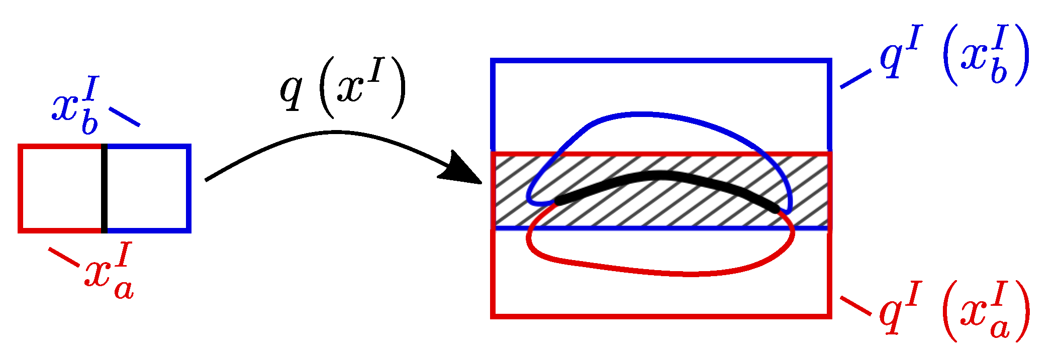
However, proving global observability solely by distinguishability using intervals is not possible. The reason is the consistent intersecting edge between two neighboring intervals that leads to an intersection in the mapping. Figure 1 illustrates this issue exemplarily. The observability function $q\left(x\right)$ is calculated for the illustrated neighboring intervals $x_a^I$ and $x_b^I$. The black line demonstrates the intersection in the mapping. Overestimation in the evaluation of the observability function leads to the fact that the interval enclosures $q^I\left(x_a^I\right)$ and $q^I\left(x_b^I\right)$ overlap mutually. The shaded area is the intersection of the two results. In the figure it can be observed that this issue even arises without overestimation.

Using condition (10) to check distinguishability facilitates the reduction of the investigation of global observability to a local problem. The justification is that only directly neighboring intervals are indistinguishable due to overestimation. A local formulation of observability for a nonlinear system is given by the following definition. To utilize this definition, the Jacobian

$$\begin{array}{c}\hfill Q\left(x\right)=\frac{\partial q\left(x\right)}{\partial x}\end{array}$$

of the observability function is introduced, which is called observability matrix.

Definition 3

(Local observability of autonomous systems for $x_0$). If $rank\left(Q\left(x\right)\right)=n$ holds for one $x\in D_x$, the system

$$\begin{array}{c}\hfill \begin{array}{cc}\hfill \dot{x}& =f\left(x\left(t\right)\right),x\left(0\right)=x_0\hfill \\ \hfill y& =h\left(x\right(t\left)\right)\hfill \end{array}\end{array}$$

is locally observable in this point x [1,19].

Definition 3 only accounts for a single point $x\in D_x$. A more general statement is stated in the following definition.

Definition 4

(Local observability of autonomous systems). If $rank\left(Q\left(x\right)\right)=n$ holds for all $x\in D_x$, the system

$$\begin{array}{c}\hfill \begin{array}{cc}\hfill \dot{x}& =f\left(x\left(t\right)\right),x\left(0\right)=x_0\hfill \\ \hfill y& =h\left(x\right(t\left)\right)\hfill \end{array}\end{array}$$

is locally observable [1,19].

To verify the condition of Definition 4, intervals are used. Thereby, the observability matrix turns into an interval matrix

$$\begin{array}{c}\hfill Q^I\left(x^I\right)={\left.\frac{\partial q\left(x\right)}{\partial x}\right|}_{x=x^I}.\end{array}$$

(11)

The nonlinear system is locally observable, if $Q^I\left(x\right)$ is full rank, such that

$$\begin{array}{c}\hfill \mathrm{rank}\left(Q^I\left(x^I\right)\right)=n.\end{array}$$

(12)

The verification of (12) is explained further in Section 2.3. The examined interval $x^I$ in (12) is the hull ${\tilde{x}}^I$ of the currently considered interval ${\check{x}}^I$ with all intervals that are indistinguishable according to condition (10). By verifying condition (12) for ${\tilde{x}}^I$, it can be proven that ${\check{x}}^I$ is locally observable in the area ${\tilde{x}}^I$. Since ${\check{x}}^I$ is locally observable in the area ${\tilde{x}}^I$ and distinguishable to all other intervals in $D_x$, all initial states $x_0\in {\check{x}}^I$ are globally observable in $D_x$. For all other intervals $x^I$ inside ${\tilde{x}}^I$, global observability cannot be proven. The reason is that ${\tilde{x}}^I$ only contains the indistinguishable intervals of ${\check{x}}^I$. For any $x^I\subset {\tilde{x}}^I$ there could exist indistinguishable intervals outside ${\tilde{x}}^I$. Hence, to prove global observability for all intervals in $D_x$, it is necessary to determine all indistinguishable intervals for every interval in $D_x$, build the respective hull and check condition (12) in each case. Note that condition (12) can only be met if ${\tilde{x}}^I$ is small enough to minimize the overestimation. If global observability for all intervals in $D_x$ can be proven by the outlined procedure, the nonlinear system is globally observable in $D_x$.

Until now, it is assumed that the system is indeed globally observable. If only a subset $\mathcal{B}\subset D_x$ happens to be observable, the conditions (10) and (12) can be used to determine $\mathcal{B}$. The observable area satisfies both conditions, whereas the other areas violate at least one of them. Additionally, the method provides all indistinguishable states. This information could be beneficial for the design of a controller. It could also be used to receive an idea about how to adapt the measurement equation to achieve global observability of the system. Further work in the field of sensor replacement can be found in [20,21].

2.3. Algorithm for Studying the Observability of Nonlinear Systems

The algorithm, which is described in the following, is represented as pseudo code in Algorithm 1. This algorithm is completely implemented in C++. To verify the observability of a nonlinear system, interval arithmetic is used. Therefore, the Interval Arithmetic Library [22] of boost [23] is necessary. Using this library, calculations with intervals are made possible by appropriate operator overloading. However, it is essential to ensure that the rounding guidelines are set correctly for the desired interval data type. The external library Eigen [24] is also used for the algorithm. Eigen is a library for linear algebra, which enables matrix and vector computation and automatic differentiation.

Algorithm1Robust observability

- INPUT: $f\left(x,\alpha \right)$, $h\left(x,\beta \right)$, $D_x$ and ${\delta }^I=\left\{{\alpha }^I,{\beta }^I\right\}$

1: generate ${\mathcal{Z}}_1$ for $D_x$ and $\delta$, store in $\mathcal{R}$  2: while$\mathcal{R}\ne \varnothing$ and $\mathrm{rad}\left(x_i^I\right)>ϵ$ do  3:    take first ${\mathcal{Z}}_i$ from $\mathcal{R}$  4:    bisect $x_i^I,{\delta }_i^I\in {\mathcal{Z}}_i$ to $x_a^I,{\delta }_a^I$ and $x_b^I,{\delta }_b^I$ and remove all connections to $x_i^I$ from $\mathcal{R}$  5:    compute $q^I\left(x_a^I\right)$ and $q^I\left(x_b^I\right)$  6:    if ${\delta }_{\mathcal{O}}^I\cap {\delta }_l^I\ne \varnothing$ with $\mathcal{O}=\left\{a,b\right\}$ then  7:       check condition (10) for both intervals with all respective intervals $x_l^I\in {\mathcal{L}}_i$ and generate the lists ${\mathcal{L}}_a$ and ${\mathcal{L}}_b$  8:    end if  9:    for $j=\left\{a,b\right\}$ do 10:       compute hulls ${\tilde{x}}_j^I$ from ${\mathcal{L}}_j$ and $x_j^I$ 11:       if condition (25) holds then 12:          remove the interval $x_j^I$ from the data structure and save it as observable 13:       else 14:          add ${\mathcal{Z}}_j$ to the list $\mathcal{R}$ 15:          add the identification number from ${\mathcal{Z}}_j$ to all ${\mathcal{Z}}_l$ from $\mathcal{R}$ according to the list ${\mathcal{L}}_j$ 16:       end if 17:    end for 18:    if necessary, adapt $\kappa$ 19: end while

2.3.1. Initialization of the Algorithm

The inputs of the algorithm are the state space representation consisting of $f\left(x,\alpha \right)$ and $h\left(x,\beta \right)$ as well the initial area $D_x$. Therefore, the initial area $D_x$ represents the set of all initial state values, which are of interest to the user.

The algorithm generates and manages two levels of lists for processing the data structure. The outer list and thus the first level is called $\mathcal{R}$ structured as a First In—First Out (FIFO) list. Since $\mathcal{R}$ manages all intervals from $D_x$, the FIFO structure provides a queue for processing the data. Thus, the intervals are bisected uniformly which is of importance for the methodology.

For efficient processing of the examined intervals, we introduce the object

$$\begin{array}{c}\hfill {\mathcal{Z}}_i=\left\{x_i^I,{\delta }_i^I,{\mathcal{L}}_i,q^I\left(x_i^I\right)\right\}.\end{array}$$

(13)

This object contains the intervals $x_i^I\subset D_x$ and ${\delta }_i^I\subset {\delta }^I$, the respective inner list ${\mathcal{L}}_i$ and the previous results of the Lie derivatives $q^I\left(x_i^I\right)$, whereby i is the identification number. The inner list ${\mathcal{L}}_i$ is one of multiple lists that together represent the second level of the data structure. Since each interval $x^I\subset D_x$ is assigned to a separate object (13), all indistinguishable intervals are assigned to the respective list $\mathcal{L}$. All these objects are stored in the outer list

$$\begin{array}{c}\hfill \mathcal{R}=\left\{{\mathcal{Z}}_r,\dots ,{\mathcal{Z}}_s\right\},r\le i\le s,r,s\in \mathbb{N}.\end{array}$$

After the data structure is established, the object ${\mathcal{Z}}_1$ is generated for the multidimensional interval $D_x$. Here the identification number is 1, since it is the first object. Furthermore, the identification numbers are assigned continuously with each newly created object. The corresponding list ${\mathcal{L}}_1$ is initially empty, since $\mathcal{L}$ never contains the identification number of the interval itself. Then ${\mathcal{Z}}_1$ is assigned to the list $\mathcal{R}$. All subsequent steps of Algorithm 1 are executed as long as the list $\mathcal{R}$ is not empty. However, the list $\mathcal{R}$ only runs empty if the nonlinear system is observable on $D_x$. If the system is not or only partially observable, the algorithm would never terminate. In this case, suitable termination criteria can be selected. For example, the smallest interval width below a threshold $ϵ$ can be used. At the beginning of each loop, the first object ${\mathcal{Z}}_i$ is taken from the list $\mathcal{R}$. Afterwards, the interval $x_i^I$ of the object ${\mathcal{Z}}_i$ is bisected along the longest edge in order to evenly scale down the intervals, successively.

2.3.2. Calculation of Lie Derivatives for Proving Distinguishability Using the Power Series

As described above, Lie derivatives are required to prove global observability. In contrast to the classic derivation, the Lie derivative of the form $L_{f}h\left(x\right)$ is the derivative of the function $h\left(x\right)$ along $f\left(x\right)$. Therefore, the number of Lie derivatives required to prove observability cannot be determined a priori. If an algorithm is used to determine and evaluate the Lie derivatives, it is necessary to establish a sufficient number of Lie derivatives in advance. This is hardly possible, since it can happen that more Lie derivatives are required than have been implemented. Thus, the determination of the observability can fail. Therefore, we reveal how an automatic determination of Lie derivatives can be performed in the following.

An alternative to the Lie derivatives is the use of the power series. The basic calculation rules are first described. For this, the base object is defined as

$$\begin{array}{c}\hfill a\left(t\right):={\displaystyle \sum _{k=0}^{\infty }}{\mathfrak{a}}_k{t}^k.\end{array}$$

(14)

Given two power series $a\left(t\right)$ and $b\left(t\right)$ according to definition (14), the calculation rules

$$\begin{array}{cc}\hfill \left(a+b\right)\left(t\right)& ={\displaystyle \sum _{k=0}^{\infty }}\left({\mathfrak{a}}_k+{\mathfrak{b}}_k\right)t^k,\hfill \end{array}$$

(15)

$$\begin{array}{cc}\hfill \left(a-b\right)\left(t\right)& ={\displaystyle \sum _{k=0}^{\infty }}\left({\mathfrak{a}}_k-{\mathfrak{b}}_k\right)t^k,\hfill \end{array}$$

(16)

$$\begin{array}{cc}\hfill \left(a·b\right)\left(t\right)& ={\displaystyle \sum _{k=0}^{\infty }}\left({\displaystyle \sum _{l=0}^k}{\mathfrak{a}}_l·{\mathbf{b}}_{k-l}\right)t^k,\hfill \\ \hfill \left(a/b\right)\left(t\right)& ={\displaystyle \sum _{k=0}^{\infty }}\left(\frac{{\mathfrak{a}}_k}{{\mathfrak{b}}_0}-\frac{1}{{\mathfrak{b}}_0}{\displaystyle \sum _{l=0}^{k-1}}\frac{{\mathfrak{a}}_0}{{\mathfrak{b}}_0}{\mathfrak{b}}_{k-l}\right)t^k\hfill \end{array}$$

(17)

follow. The corresponding power series expressions can also be created for other mathematical functions, such as trigonometric functions. For simplicity, these are not described. To combine the power series with the Lie derivatives, the state $x\left(t\right)$ is described as a power series

$$\begin{array}{c}\hfill x\left(t\right)={\displaystyle \sum _{k=0}^{\infty }}{\mathfrak{x}}_k{t}^k\end{array}$$

according to definition (14). Thus, it follows for the state equations

$$\begin{array}{c}\hfill f\left(x\left(t\right)\right)={\displaystyle \sum _{k=0}^{\infty }}{\mathfrak{f}}_k{t}^k.\end{array}$$

(18)

For the ordinary differential equation of the nonlinear system, it follows that

$$\begin{array}{c}\hfill \dot{x}\left(t\right)={\displaystyle \sum _{k=0}^{\infty }}{\mathfrak{x}}_{k+1}\left(k+1\right)t^k.\end{array}$$

(19)

Inserting (19) in (18) yields

$$\begin{array}{c}\hfill {\mathfrak{x}}_{k+1}=\frac{1}{k+1}{\mathfrak{f}}_k,\end{array}$$

(20)

with ${\mathfrak{f}}_k=f\left({\mathfrak{x}}_0,{\mathfrak{x}}_1,\dots ,{\mathfrak{x}}_k\right)$ and $x\left(0\right)={\mathfrak{x}}_0$. Furthermore, if the output equation (2) is formulated by the power series

$$\begin{array}{c}\hfill y\left(t\right)={\displaystyle \sum _{k=0}^{\infty }}{\mathfrak{y}}_k{t}^k,\end{array}$$

(21)

the Taylor series coefficients of equation (6) can be determined. Therefore, the coefficients ${\mathfrak{y}}_k={\mathfrak{h}}_k$ with ${\mathfrak{h}}_k=h\left({\mathfrak{x}}_0,{\mathfrak{x}}_1,\dots ,{\mathfrak{x}}_k\right)$ are required. Consequently, the definition (21) is used together with the Taylor series from equation (6) and

$$\begin{array}{c}\hfill {\mathfrak{y}}_k=\frac{1}{k!}{L}_f^{k}h\left(x_0\right)\end{array}$$

(22)

holds for each of the coefficients. Inserting ${\mathfrak{y}}_k={\mathfrak{h}}_k$ into (22) yields the Lie derivatives

$$\begin{array}{c}\hfill L_f^{k}h\left(x_0\right)=k!{\mathfrak{h}}_k.\end{array}$$

(23)

Thus, it is possible to determine the value of any Lie derivative without computing its analytic expression. This procedure can be implemented as an algorithm. Additionally, both automatic differentiation and interval arithmetic can be applied. Consequently, it becomes possible to calculate the solution set of Lie derivatives over a whole range of the values of $x_0$. Simultaneously, the values of the Jacobian can also be determined by using automatic differentiation. Note that the calculation of the Lie derivatives as well as the interval observability matrix (11) is performed accordingly even if the nonlinear system has uncertainties. The system uncertainties are described as a bounded interval in the nonlinear system equations. Using IA automatically considers these uncertainties and the calculation of both (8) and (11) can be executed as per description.

2.3.3. Example: Direct Calculation of Lie Derivatives

Let us assume the nonlinear system

$$\begin{array}{c}\hfill f\left(x\right)=\left(\begin{array}{c}{x}_2\\ -x_1+x_1^2{x}_2\end{array}\right)\end{array}$$

(24)

with the initial point $x\left(0\right)={\mathfrak{x}}_0={\left(24\right)}^{\mathrm{T}}$ and the output function

$$h\left(x\right)=x_1+x_2^3.$$

The first two Lie derivatives are

$$\begin{array}{cc}\hfill L_f^{0}h\left(x\right)& =x_1+x_2^3\hfill \\ \hfill L_f^{1}h\left(x\right)& =x_2-3x_1{x}_2^2+3x_1^2{x}_2^3\hfill \end{array}$$

and with $x\left(0\right)$ yields $L_f^{0}h\left(x\right)=66$ and $L_f^{1}h\left(x\right)=676$. To obtain the same results with an automatic iterative calculation first ${\mathfrak{x}}_1$ according to (20) is necessary. Thus, we obtain ${\mathfrak{f}}_0={\left(414\right)}^{\mathrm{T}}$ by inserting ${\mathfrak{x}}_0$ in (24) and according to (20) ${\mathfrak{x}}_1={\left(414\right)}^{\mathrm{T}}$. Now we can utilize (23) to obtain the same results by computing $h\left({\mathfrak{x}}_0\right)$ and $h\left({\mathfrak{x}}_0,{\mathfrak{x}}_1\right)$, whereby, $h\left({\mathfrak{x}}_0,{\mathfrak{x}}_1\right)$ can be computed by the calculation rules (15)–(17). With this method, all further Lie derivatives can be computed iteratively with (20) and (23) without calculating the Lie derivatives analytically. Using the power series arithmetic, any number of values of the Lie derivatives can be calculated without a single analytically determined Lie derivative.

2.3.4. Applying the Local Condition

After calculating the Lie derivatives $q^I\left(x_a^I\right)$ and $q^I\left(x_b^I\right)$, condition (10) is checked. If the algorithm is in any iteration, the original list ${\mathcal{L}}_i$ is not empty. In the previous iterations it could already be ensured that $x_i^I$ is indistinguishable from all intervals in the list. Therefore, $x_a^I$ and $x_b^I$ only need to be checked against the intervals located in the list. This results in lists ${\mathcal{L}}_a$ and ${\mathcal{L}}_b$. The hope here is that the bisection will reduce the overestimation, whereby areas can be distinguished from $D_x$, which were previously indistinguishable. As already explained, the condition (10) alone cannot be used to numerically prove the observability of nonlinear systems. It is therefore necessary to refer to the local conditions. First it is necessary to form the hull of all intervals of the list ${\mathcal{L}}_j$ with the interval $x_j^I$ for $j=a,b$. To check the local condition (12), the interval observability matrix $Q^I\left({\tilde{x}}_j^I\right)$ must be calculated. This requires the Jacobian. By using the automatic differentiation provided in the program library Eigen, the value of the matrix $Q^I\left({\tilde{x}}_j^I\right)$ can be determined without having to analytically set up the Jacobian. The rank is then checked. If the matrix $Q^I\left({\tilde{x}}_j^I\right)$ has full rank, it can be proven that the states enclosed by the corresponding interval $x_j^I$ are globally observable on $D_x$. However, if the full rank of the matrix $Q^I\left({\tilde{x}}_j^I\right)$ is not detectable for the currently considered hull ${\tilde{x}}_j^I$, the corresponding interval $x_j^I$ cannot be discarded yet. The interval observability matrix is a matrix of dimension $\left(n\times \kappa p\right)$, where n represents the number of system states, $\kappa$ the number of Lie derivatives and p the dimension of the output. To observe all states, $\kappa$ is selected so that $\kappa p\ge n$ applies. Consequently, the maximum rank of the interval observability matrix $Q^I\left({\tilde{x}}_j^I\right)$ is equal to n. The exact rank of the matrix is not of importance for the local condition (12), only whether the rank is full. A suitable method for checking the rank is to examine the estimated eigenvalues. For this purpose, the method from Rohn from [25] offers a possibility to enclose these eigenvalues as sharply as possible using an interval. The precondition is that the interval matrix is a square matrix. Accordingly, the quadratic interval matrix is defined with the dimension $\left(\left(n+\kappa p\right)\times \left(n+\kappa p\right)\right)$ as

$$V^I:=\left(\begin{array}{cc}0& Q^I\left({\tilde{x}}_j^I\right)\\ Q^I{\left({\tilde{x}}_j^I\right)}^{\mathrm{T}}& 0\end{array}\right).$$

Using Rohn’s theorem from [25], the interval eigenvalues of the matrix $V^I$ can be enclosed. The second theorem of Rohn from [25] states that the eigenvalues of an interval matrix are enclosed by

$${\lambda }_i^I\left(V^I\right)\subseteq \left[{\lambda }_i\left(\mathrm{mid}\left(V^I\right)\right)-\rho \left(\mathrm{rad}\left(V^I\right)\right),{\lambda }_i\left(\mathrm{mid}\left(V^I\right)\right)+\rho \left(\mathrm{rad}\left(V^I\right)\right)\right].$$

Here, $\rho$ is the spectral radius of the matrix $\mathrm{rad}\left(V^I\right)$, whose radius is determined for all entries according to Equation (4). The singular values of matrix $Q^I\left({\tilde{x}}_j^I\right)$ are related to the eigenvalues of matrix $V^I$. Therefore, it is sufficient to verify that $2n$ eigenvalues of matrix $V^I$ are non-zero to demonstrate the full rank of the interval observability matrix $Q^I\left({\tilde{x}}_j^I\right)$. Consequently, the local condition can be rewritten with the theorem of Rohn [25] to the condition

$$\left\{\lambda \left(\mathrm{mid}\left(V^I\right)\right)|\left|\lambda \left(\mathrm{mid}\left(V^I\right)\right)\right|-\rho \left(\mathrm{rad}\left(V^I\right)\right)>0\right\}=2n.$$

(25)

If it can be determine by condition (25) that $2n$ of the $n+\kappa p$ eigenvalues are non-zero then the interval observability matrix $Q^I\left({\tilde{x}}_j^I\right)$ is full rank. The Jacobian Conjecture states that the inverse of a function exists if the rank condition (12) is fulfilled. Although the local condition (12) is a commonly used criterion for observability, the Jacobian Conjecture is not definitively proven for the case $n>1$ and is considered one of the greatest mathematical problems of the century [26].

2.3.5. Final Remarks

The interval observability matrix $Q^I\left({\tilde{x}}_j^I\right)$ includes many more matrices than the Jacobian matrices because it uses intervals. Furthermore, all matrices in between, which are not Jacobians themselves, are included. If an interval ${\tilde{x}}^I$ meets condition (25), it means that all possible matrices meet this condition instead of solely all Jacobians. This can basically be reduced to the mean value theorem. Assume two points $x,y\in {\tilde{x}}^I$ then

$$q\left(x\right)-q\left(y\right)=\underset{M}{\underbrace{\left[\begin{array}{c}{\left(\frac{\partial q_i\left({\xi }_1\right)}{\partial x}\right)}^{\mathrm{T}}\\ {\left(\frac{\partial q_i\left({\xi }_2\right)}{\partial x}\right)}^{\mathrm{T}}\\ ⋮\end{array}\right]}}\left(x-y\right)$$

for ${\xi }_i$ in between x and y. If this is done for all points out of ${\tilde{x}}_j^I$ then all matrices $M\in M^I$, due to the usage of IA. Therefore, condition (12) test the interval matrix $M^I$ since

$$M^I={\left.\frac{\partial q\left(x\right)}{\partial x}\right|}_{x={\tilde{x}}_j^I}.$$

Thus, if the interval observability matrix $Q^I\left({\tilde{x}}_j^I\right)$ is proven to be full rank, a more strict requirement is already fulfilled by condition (25) due to the interval arithmetic. Consequently, the local rank condition represents a clearly secured condition for checking the observability.

The last step of the algorithm in each iteration is to determine the number of Lie derivatives $\kappa$ to be calculated. There is no method for determining the required number of Lie derivatives for any nonlinear system in advance and for proving observability. However, the numerical approach to determining observability offers the flexibility to vary the number of Lie derivatives. To achieve this, the algorithm always calculates one more Lie derivative than is currently necessary. The minimum number is specified by the system dimension. Both the test of the condition (10) to determine distinctness and the examination of the rank by means of the condition (25) are performed with comparatively less numerical effort. If it turns out that one or both conditions can be fulfilled with more Lie derivatives, the number of Lie derivatives is incremented for the next iteration. Whenever possible, the number of Lie derivatives required is reduced to increase the efficiency of the algorithm. However, if no interval over a larger number of Lie derivatives ever meets either condition, the number of Lie derivatives is also increased successively.

3. Results of the Algorithm

In this section, the algorithm presented above will be evaluated by three examples. The examples should offer a better understanding of the methodology and point out individual aspects separately. Therefore, there are no system uncertainties in the first two considered examples in order to emphasize specific advantages of the method without being distracted by the interval parameters. All examples are executed on a standard 64 bit computer with i7-8700 @3.20GHz and 16GB RAM with a non-real-time operating system.

3.1. Example 1

The first example is taken from [11]. The nonlinear system is given by

$$\begin{array}{ccc}f\left(x\right)& =& \left(\begin{array}{c}-x_2^{}+x_1^{}\left(1-x_1^2-x_2^2\right)\\ \phantom{-}{x}_1^{}+x_2^{}\left(1-x_1^2-x_2^2\right)\\ -x_3^{}\left(x_1^2+x_2^2\right)\end{array}\right)\\ h\left(x\right)& =& x_1^2+x_2^2+x_3^2.\end{array}$$

(26)

According to [11], this system is non observable. To verify the algorithm presented in the previous section, the observability is examined using the presented method. Therefore, the system is analyzed on the set

$$D_x=\left(\begin{array}{c}\left[-11\right]\\ \left[-11\right]\\ \left[-11\right]\end{array}\right).$$

After 16 days, 5 h, 18 min and 30 s no globally observable interval could be identified. During this time, 75,000 iterations have been executed. The long computing time and small amount of iterations implies that the system (26) is not observable. The small amount of iterations also implies that the lists ${\mathcal{L}}_i$ contain several intervals. Hence, numerous intervals are indistinguishable from one another.

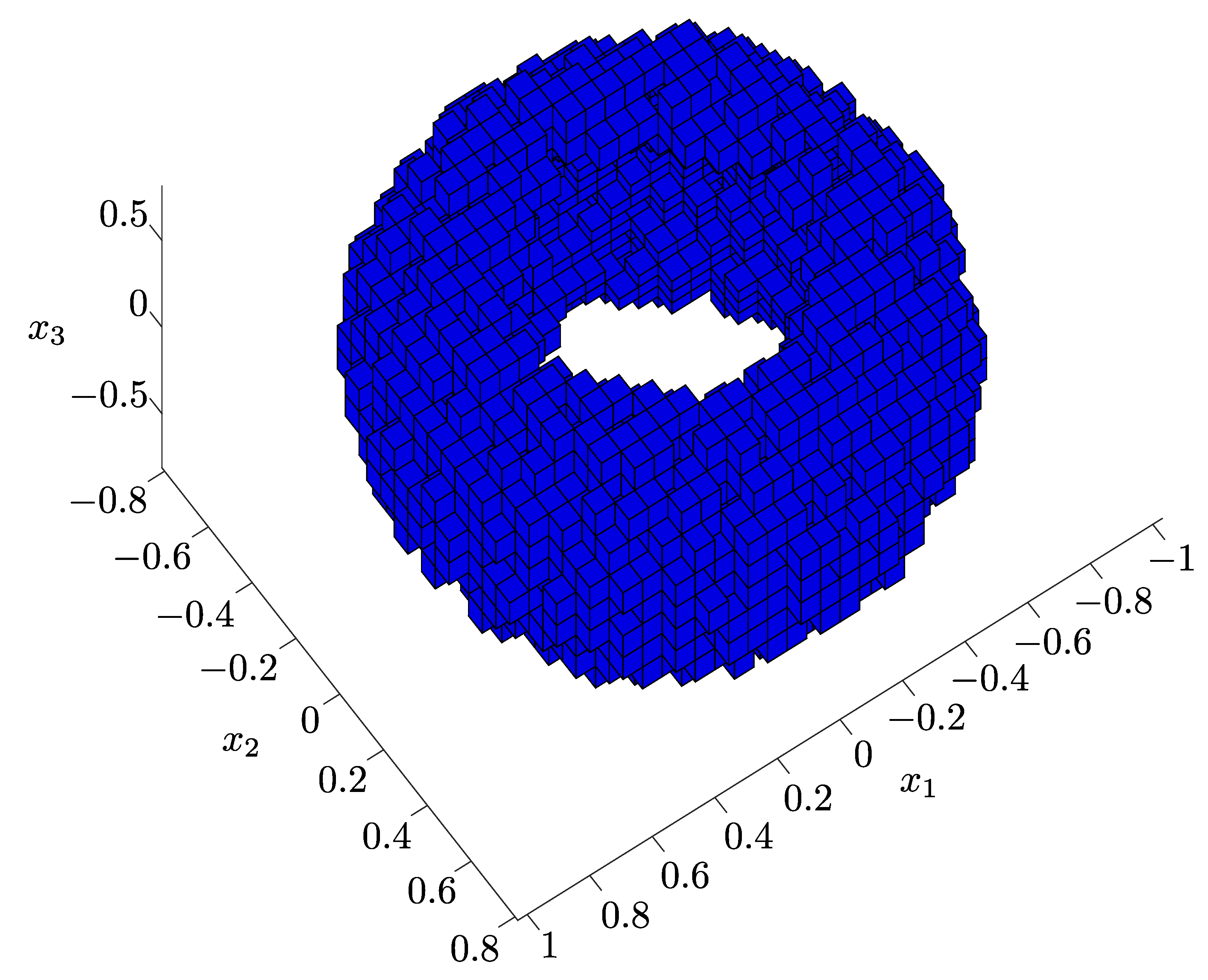
Additionally to the statement that the system is non observable, the presented method is capable of providing the set of states that are indistinguishable from a specific initial state. This is exemplarily demonstrated in Figure 2. All blue intervals are indistinguishable from the initial state

$$x^I=\left(\begin{array}{ll}[-0.5\phantom{000}& -0.4375]\\ [-0.4375& -0.375\phantom{0}]\\ [\phantom{\mathrm{-}}0.3125& \phantom{\mathrm{-}}0.375\phantom{0}]\end{array}\right),$$

(27)

which is located inside the blue torus of indistinguishable intervals. The shape of a torus results from the quadratic terms in the measurement equation $h\left(x\right)$ and the recurring terms within the system equations $f\left(x\right)$. Additionally, overestimation expands the shape. The figure illustrates an example after 10,000 iterations. After further iterations, the structure of indistinguishable intervals keeps its shape, however, the torus is enclosed more sharply.

The information about the set of states that are indistinguishable from another state can be used during the design phase of a plant. Information can be derived on how to adapt the measurement equation to make the system observable. In the provided example, the shape of a torus suggests that the quadratic terms in the measurement equation $h\left(x\right)$ should be avoided. Other methods are not able to provide this type of information. For example, in [11] only non-observability could be identified.

3.2. Example 2

In the following, a system with trigonometric functions shall be examined on observability. Therefore, the nonlinear system

$$\begin{array}{ccc}f\left(x\right)& =& \left(\begin{array}{c}cos\left(x_2+\frac{1}{2}\right)\\ sin\left(x_1\right)\end{array}\right)\\ h\left(x\right)& =& x_1^3+\frac{1}{2}{x}_2^2.\end{array}$$

(28)

is considered. The observability is examined on the set

$$D_x=\left(\begin{array}{c}\left[-1010\right]\\ \left[-1010\right]\end{array}\right).$$

(29)

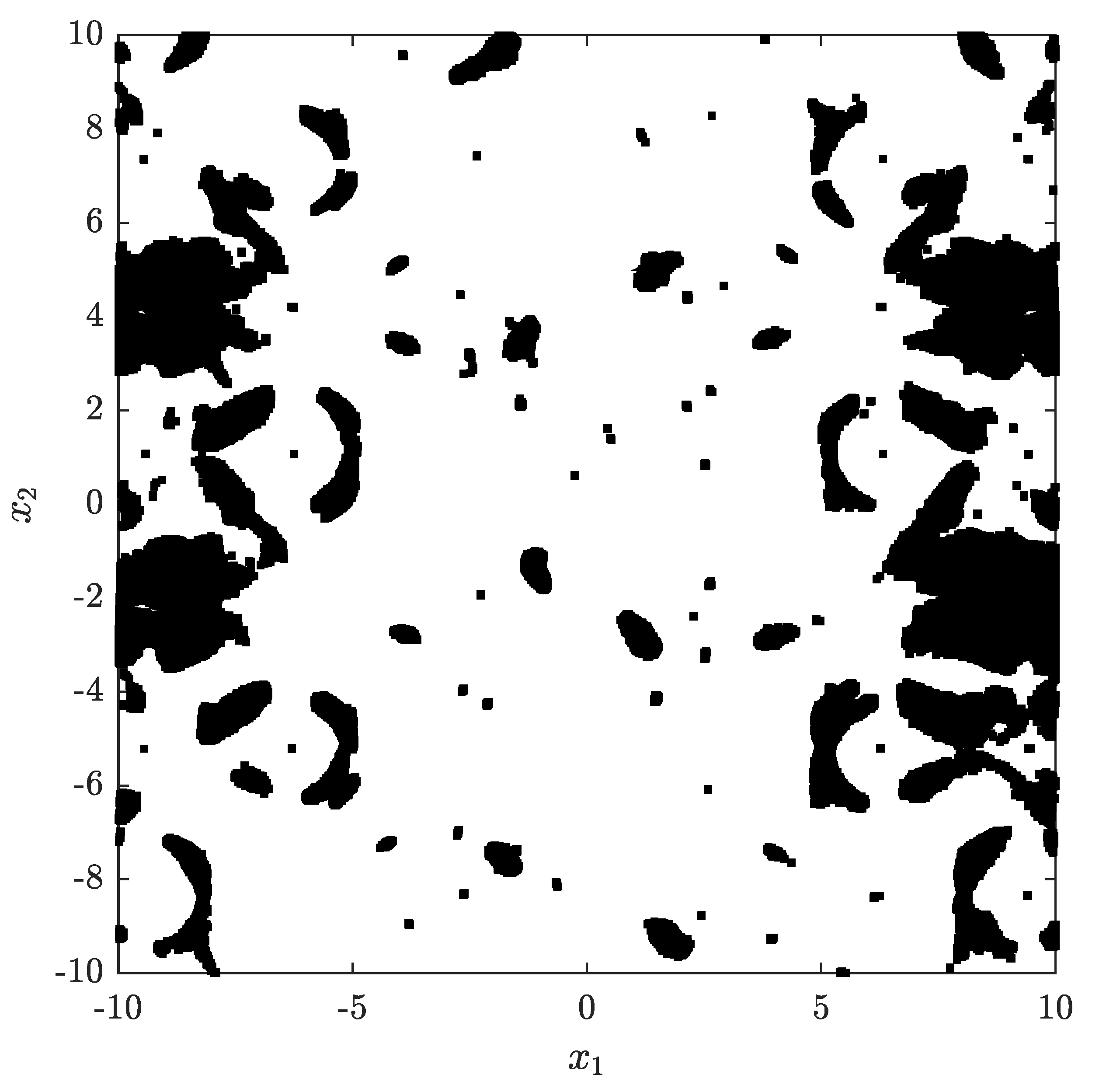
Figure 3 demonstrates all intervals in black, in which global observability could not be proven after 691,000 iterations. These iterations take a computing time of 3 d, 5 h, 42 min and 43 s to prove that 89.186% of the initial $D_x$ (29) is observable. However, most of the computational time is spent for the last 63,000 iterations. After 628,000 iterations and 528.084 s 88.266% of the initial $D_x$ (29) already have been proven to be observable. This highly increase in the computational time and the few areas for which observability could been additionally proven suggest that most of the black areas of Figure 3 are indeed indistinguishable. This is due to the fact that the lengths of the lists ${\mathcal{L}}_i$ increase, as the number of indistinguishable intervals for each interval increases. This increase in the number of indistinguishable intervals may indicate that the black areas of Figure 3 are not globally observable on $D_x$. The example reveals that the presented method is able to find rather complex structures, that cannot be represented by simple conditions.

3.3. Example 3

The state space representation from [13] is given by

$$\begin{array}{ccc}f\left(x,a\right)& =& \left(\begin{array}{c}{x}_2\left(x_2+a\right)\\ x_2\end{array}\right)\\ h\left(x\right)& =& x_1\end{array}$$

(30)

with the system uncertainty a. The observability of system (30) has been investigated in [13] using quantifier elimination. Using the presented algorithm, the observability is examined on the set

$$D_x=\left(\begin{array}{c}\left[-55\right]\\ \left[-55\right]\end{array}\right)$$

(31)

and the system uncertainty is limited to $a^I=[-11]$. After 42,500,000 iterations, all intervals for which global observability is not yet provable on (31) have an uncertainty of $a^I=[-0.08593750.0703125]$. All other intervals could be removed from the list $\mathcal{R}$ indicating that the system is globally observable there. The computing time for the number of iterations is 20 h, 58 min and 9 s. Further iterations reduce the area $a^I$ of the intervals that remain in $\mathcal{R}$. This result corresponds to the result in [13]. There, the system is observable for $a\ne 0$, if the first three Lie derivatives are calculated.

3.4. Remark to the Presented Examples

In all three examples the investigated set $D_x$ is of the same magnitude in every component of the state vector. If, for a nonlinear system the observability has to be determine for which one component of the state vector has a magnitude several decades higher than an other component due to a different physical unit, then this would be troublesome. The algorithm would need to bisect the component with higher magnitude many times to reduce the overestimation. This would result in a colossal growth of the list structure and slow the algorithm. To counteract this, an initial normalization of the state domain would be necessary.

4. Discussion

As elaborated in the previous section, the presented method provides three main advantages. Firstly, the algorithm is capable of determining which initial states cannot be distinguished from which particular initial state in the case that the system is not entirely observable on a given set. This can provide further understanding why a given system is not entirely observable. Thus, the method supports the designing of a technical system by providing information on how to modify the output function in order to achieve global observability on the desired state space. Hence, the usage of different sensors can be checked whether they provide observability. Secondly, the algorithm delivers the initial states, which are observable on $D_x$ and which are probably not. Therefore, if the nonlinear system is only observable on a subset $\mathcal{B}\subset D_x$, this subset $\mathcal{B}$ can be determined. This is the case even if the subset $\mathcal{B}$ is of a complex structure. Thirdly, the algorithm is capable of considering system uncertainties and can determine the observability in dependency of these uncertainties. This is particularly useful if parameters of the system are unknown or the measurement function contains design parameters due to different types of sensors that could be used. From the results it is possible to extract which sensors benefit the observability of the states that are of interest for the user. This is mostly archived by the interval based numerical approach. Furthermore, interval based methods deliver guaranteed results and are robust against rounding errors [17].

The runtime of the algorithm highly depends on the considered nonlinear system and whether the states are observable or not. This was especially noticeable in Example 2. For an increase of 0.92% over 3 d and 5 h of computational time was necessary, while the first 628,000 iterations only took 8 min and 48.084 s. This drastic increase of computational time per iteration occurs when the initial states are indistinguishable. In that case, the list of the objects (13) grows for many elements by every iteration, which slows the algorithm down. Nonetheless, in case of complex nonlinear systems, an adaptation of the algorithm to parallelize the execution might be worthwhile to enhance the performance. However, the determination whether the nonlinear system is observable is a task that needs to be done once before the technical system is used. Therefore, the runtime of the method is not of immediate importance. The here presented work aims to demonstrate the benefits of interval based numerical approaches.

References

- Hermann, R.; Krener, A. Nonlinear controllability and observability. IEEE Trans. Autom. Control. 1977, 22, 728–740. [Google Scholar] [CrossRef] [Green Version]
- Ding, S.; Chen, W.; Mei, K.; Murray-Smith, D.J. Disturbance Observer Design for Nonlinear Systems Represented by Input–Output Models. IEEE Trans. Ind. Electron. 2020, 5, 1222–1232. [Google Scholar] [CrossRef] [Green Version]
- Fliess, M. A remark on nonlinear observability. IEEE Trans. Autom. Control. 1982, 27, 489–490. [Google Scholar] [CrossRef]
- Brockett, R.W. Nonlinear Systems and Nonlinear Estimation Theory. In Stochastic Systems: The Mathematics of Filtering and Identification and Applications. NATO Advanced Study Institutes Series (Series C—Mathematical and Physical Sciences); Springer: Dordrecht, The Netherlands, 1981; pp. 441–477. [Google Scholar]
- Tibken, B. Observability of nonlinear systems–An algebraic approach. In Proceedings of the 2004 43rd IEEE Conference on Decision and Control (CDC) (IEEE Cat. No. 04CH37601), Nassau, Bahamas, 14–17 December 2004; pp. 4824–4825. [Google Scholar]
- Kawano, Y.; Ohtsuka, T. Global observability of polynomial systems. In Proceedings of the SICE Annual Conference, Taipei, Taiwan, 18–21 August 2010; pp. 2038–2041. [Google Scholar]
- Zeng, S.; Allgöwer, F. On the ensemble observability problem for nonlinear systems. In Proceedings of the 2015 54th IEEE Conference on Decision and Control (CDC), Osaka, Japan, 15–18 December 2015; pp. 6318–6323. [Google Scholar]
- Zeng, S. On the Ensemble Observability of Dynamical Systems. Ph.D. Thesis, Institut für Systemtheorie und Regelungstechnik, University of Stuttgart, Stuttgart, Germany, 2016. [Google Scholar]
- Lagrange, S.; Delanoue, N.; Jaulin, L. Guaranteed Numerical Injectivity Test via Interval Analysis. In Trends in Constraint Programming; ISTE: London, UK, 2017; pp. 233–244. [Google Scholar]
- Lagrange, S.; Delanoue, N.; Jaulin, L. On sufficient conditions of the injectivity: Development of a numerical test algorithm via interval analysis. Reliable Comput. 2007, 13, 409–421. [Google Scholar] [CrossRef]
- Röbenack, K.; Reinschke, K.J. An efficient method to compute Lie derivatives and the observability matrix for nonlinear systems. In Proceedings of the International Symposium on Nonlinear Theory and Applications (NOLTA), Dresden, Germany, 17–21 September 2010; pp. 625–628. [Google Scholar]
- Rauh, A.; Minisini, J.; Hofer, E. Verification Techniques for Sensitivity Analysis and Design of Controllers for Nonlinear Dynamic Systems with Uncertainties. Int. J. Appl. Math. Comput. Sci. 2009, 19, 425–439. [Google Scholar] [CrossRef]
- Röbenack, K.; Voßwinkel, R. Formal Verification of Local and Global Observability of Polynomial Systems Using Quantifier Elimination. In Proceedings of the 2019 23rd International Conference on System Theory, Control and Computing (ICSTCC), Sinaia, Romania, 9–11 October 2019; pp. 314–319. [Google Scholar]
- Tarski, A. A Decision Method for Elementary Algebra and Geometry. In Quantifier Elimination and Cylindrical Algebraic Decomposition. (A Series of the Research Institute for Symbolic Computation, Johannes-Kepler-University, Linz, Austria); Springer: Vienna, Austria, 1998. [Google Scholar]
- Paradowski, T.; Tibken, B.; Swiatlak, R. An Approach to Determine Observability of Nonlinear Systems Using Interval Analysis. In Proceedings of the 2017 American Control Conference (ACC), Seattle, WA, USA, 24–26 May 2017; pp. 3932–3937. [Google Scholar]
- Paradowski, T. Intervallarithmetische Untersuchung der Beobachtbarkeit und Zustandsschätzung nichtlinearer Systeme. Ph.D. Thesis, Faculty of Electrical, Information and Media Engineering, University of Wuppertal, Wuppertal, Germany, 2020. Submitted. [Google Scholar]
- Moore, R.E.; Kearfott, R.B.; Cloud, M.J. Introduction to interval analysis. In Society for Industrial and Applied Mathematics; SIAM: 3600 University City Science Center Philadelphia, PA, USA, 2009. [Google Scholar]
- Jaulin, L.; Kieffer, M.; Didrit, O.; Walter, É. Applied Interval Analysis; Springer: London, UK, 2001. [Google Scholar]
- Röbenack, K. Nichtlineare Regelungssysteme; Springer: Vieweg, Germany, 2017. [Google Scholar]
- Frisk, E.; Krysander, M. Sensor placement for maximum faultisolability. In Proceedings of the 18th International Workshop on Principles of Diagnosis (DX-07), Nashville, TN, USA, 29–31 May 2007. [Google Scholar]
- Raissi, T.; Efimov, D.; Zolghadri, A. Interval State Estimation for a Class of Nonlinear Systems. IEEE Trans. Autom. Control. 2012, 57, 260–265. [Google Scholar] [CrossRef]
- Brönnimann, H.; Melquiond, G.; Pion, S. The design of the Boost interval arithmetic library. Theor. Comput. Sci. 2006, 351, 111–118. [Google Scholar] [CrossRef] [Green Version]
- The Boost C++ Libraries. Available online: http://www.boost.org/ (accessed on 24 January 2020).
- Eigen. Eigen C++ Librarie. Available online: http://eigen.tuxfamily.org/ (accessed on 24 January 2020).
- Rohn, J. Bounds on Eigenvalues of Interval Matrices. J. Appl. Math. Mech. 1998, 78, 1049–1050. [Google Scholar] [CrossRef] [Green Version]
- Smale, S. Mathematical Problems for the Next Century. The Math. Intell. 1998, 20, 7–15. [Google Scholar] [CrossRef]
Figure 1.
Overestimation of adjacent intervals in the mapping area. Common edge (illustrated in black) leads to an overlapping (illustrated as black shaded area).
Figure 2.
Illustration of all indistinguishable intervals for the interval (27) after 10,000 iterations for the nonlinear system (26).
© 2020 by the authors. Licensee MDPI, Basel, Switzerland. This article is an open access article distributed under the terms and conditions of the Creative Commons Attribution (CC BY) license (http://creativecommons.org/licenses/by/4.0/).
Share and Cite
MDPI and ACS Style
Paradowski, T.; Lerch, S.; Damaszek, M.; Dehnert, R.; Tibken, B. Observability of Uncertain Nonlinear Systems Using Interval Analysis. Algorithms 2020, 13, 66. https://0-doi-org.brum.beds.ac.uk/10.3390/a13030066
AMA Style
Paradowski T, Lerch S, Damaszek M, Dehnert R, Tibken B. Observability of Uncertain Nonlinear Systems Using Interval Analysis. Algorithms. 2020; 13(3):66. https://0-doi-org.brum.beds.ac.uk/10.3390/a13030066
Chicago/Turabian StyleParadowski, Thomas, Sabine Lerch, Michelle Damaszek, Robert Dehnert, and Bernd Tibken. 2020. "Observability of Uncertain Nonlinear Systems Using Interval Analysis" Algorithms 13, no. 3: 66. https://0-doi-org.brum.beds.ac.uk/10.3390/a13030066
Note that from the first issue of 2016, this journal uses article numbers instead of page numbers. See further details here.