Two-Step Classification with SVD Preprocessing of Distributed Massive Datasets in Apache Spark

Abstract

At the dawn of the 10V or big data data era, there are a considerable number of sources such as smart phones, IoT devices, social media, smart city sensors, as well as the health care system, all of which constitute but a small portion of the data lakes feeding the entire big data ecosystem. This 10V data growth poses two primary challenges, namely storing and processing. Concerning the latter, new frameworks have been developed including distributed platforms such as the Hadoop ecosystem. Classification is a major machine learning task typically executed on distributed platforms and as a consequence many algorithmic techniques have been developed tailored for these platforms. This article extensively relies in two ways on classifiers implemented in MLlib, the main machine learning library for the Hadoop ecosystem. First, a vast number of classifiers is applied to two datasets, namely Higgs and PAMAP. Second, a two-step classification is ab ovo performed to the same datasets. Specifically, the singular value decomposition of the data matrix determines first a set of transformed attributes which in turn drive the classifiers of MLlib. The twofold purpose of the proposed architecture is to reduce complexity while maintaining a similar if not better level of the metrics of accuracy, recall, and $F1$. The intuition behind this approach stems from the engineering principle of breaking down complex problems to simpler and more manageable tasks. The experiments based on the same Spark cluster indicate that the proposed architecture outperforms the individual classifiers with respect to both complexity and the abovementioned metrics.

1. Introduction

In the big data era, the major drivers behind redefining application paradigms are the need for efficient and reliable distributed computing frameworks as well as the ability to handle large data volumes collected from fields so diverse as smart cities, digital health care, high resolution navigation systems, and digital cultural heritage. In addition, the need for the development of programming languages which take into account both the defining characteristics of these frameworks and the recent lessons about defensive programming, code readability and maintenance, and version control in an abstract and programmer friendly manner, must also be taken into account. Such is the case of the Apache Spark framework, a significant part of the Hadoop ecosystem along with Kafka, in order to build streaming platforms and Hive aiming to manage data in relational databases, in conjunction with Scala. The latter is a multi-paradigm (functional and object-oriented) programming language with a strong static type system running on top of the JVM ecosystem. Moreover, PySpark, namely the Spark Python API, has remarkable success since it provides Python functionality for Spark Resilient Distributed Datasets ($RDDs$), the main Spark data abstraction type.

Among machine learning ($ML$) tasks, classification stands out as one of the most computationally intensive ones. This can be attributed not only to the massive data volume driving the advanced ML models but also to the time required to fetch a specific batch with dynamically formed or even ad hoc queries involving thousands of rows. Moreover, in the big data era, even elementary operations, such as a single inner product or a hash mapping, may require additional time because of the number of operands involved and their distribution across the shared file system. In addition, the iterative training process of most classifiers results in a high number of computations. Even evaluating a loss function may take a significant portion of the total computations in some very rare cases. In order to improve performance, feature selection or transformation can take place before the actual classification. Although this preprocessing step requires time, the resulting feature set may contain considerably less attributes which may further represent the various classes in an easily separable way. In turn, this leads to a more efficient classification process in terms of both accuracy and total computation time.

The primary research objective of this article is twofold. Firstly, the two-step feature selection and classification methodology is described. As a preprocessing step, the singular value decomposition ($SVD$) has been selected as it efficiently identifies eigenfeatures hidden in massive datasets. As stated in our previous work, learning new data features while preserving old data features can be considered as one of the most important goal of incremental learning methods [1]. Secondly, the results of the proposed methodology applied to a considerable number of real and synthetic datasets using the Apache Spark MLlib, a machine learning library optimized for distributed systems which provides among others the SVD functionality, are discussed. Several classification models such as decision trees, random forest, and logistic regression, have been investigated and their performance in terms of precision, recall and $F1$ metric, as the dataset size varies, has been recorded. As a secondary objective, the specifics of the Spark system, along with the PySpark and the SparkQL modules developed in order to perform the two-step classification, are outlined.

The principal motivation behind this article is to show the potential of preprocessing in a typical data science pipeline. Additionally, the distributed nature of Apache Spark makes the preprocessing step considerably easier, thus gaining valuable insight into the attribute space with comparatively low complexity.

The remainder of this work is structured as follows. Section 2 briefly overviews the relevant scientific literature and various cloud computing methodologies. Section 3 presents the classification algorithms available by MLlib and used in the proposed approach along with the proposed methodology. Section 4 discusses the training steps, the analysis cases as well as the two datasets used. Moreover, Section 5 describes the evaluation experiments conducted and comments on the results. Finally, Section 6 recapitulates the main conclusions and draws directions for future work. Matrices are represented by boldface uppercase and vectors by boldface lowercase, whereas ordinary lowercase are reserved for scalars.

2. Related Work

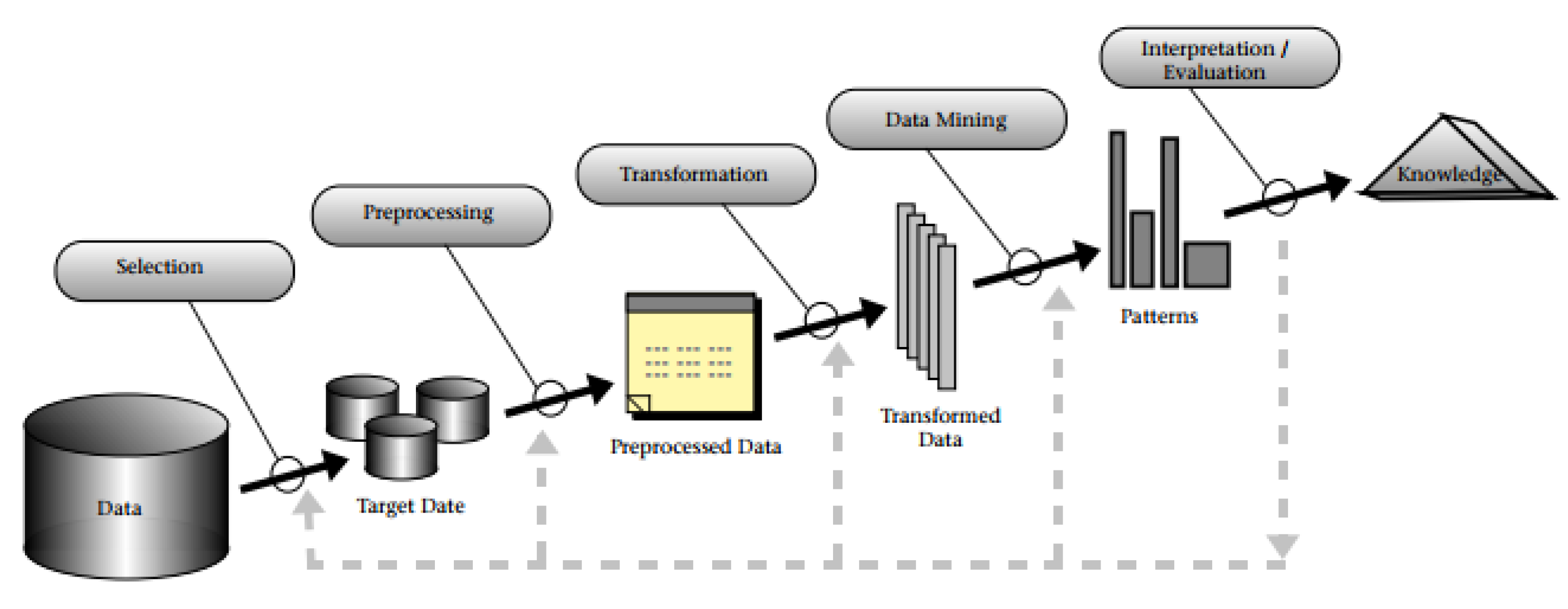
2.1. Data Mining and Two-Step Classification

The field of data mining came into existence relatively recently with the stated objective of systemizing the methodologies for extracting hidden patterns or other knowledge of interest from massive datasets. For instance, data mining provides the tools for discovering latent correlations between features, thus allowing feature transformation and dimensionality reduction [2]. Both are crucial in the extract-transform-load ($ETL$) cycle in databases. As stated in [3], the knowledge discovery has a wide range of applications, with marketing, finance and fraud detection defining a portion of them. The process of knowledge discovery is structured in several stages, the first of which is feature selection, as presented in Figure 1. The preprocessing and transformation steps follow and lead to the main stage of data mining, where a suitable algorithm or an ad hoc version of it, extracts latent information in a form appropriate for future use [4].

Data mining consists of various tasks, most notably visualization, cleansing, missing value completion, outlier discovery, clustering, dimensionality reduction, and classification. In its most basic form, the latter consists of assigning labels taken from a finite set to algorithmic objects, for instance graphs, vectors or countable sequences, based on a small number of known label-object pairings. A methodological approach to classification stems from the common engineering intuition to dividing hard optimization problems to simpler subtasks in order to obtain a solution. The classification techniques based on this approach are many and diverse. In the Gauss-Dantzig selector, linear programming performs very sparse model selection under certain inequality constraints and then ordinary least squares estimate the values of the model coefficients [5,6]. Another prime example constitutes the generic scheme proposed in [7] for clustering objects stored in GIS databases, where in each clustering iteration, there is a step dependent only on non-spatial attributes followed by a step where the location-based operations are executed. In addition, in [8], a methodology for deduplicating records in databases in an unsupervised way is described, where synthetic high quality records are created based on the underlying domain and subsequently they are driven to a high performing classifier such as a support vector machine (SVM). In [9], an expectation-maximization ($EM$)-like clustering algorithm for fuzzy data based on belief functions is implemented and compared to one-step fuzzy classifiers. Finally, an implicit two-step spatiosocial clustering of trilingual tweets is proposed in [10], where a genetic algorithm takes into account both linguistic similarity and spatial proximity models. Other applications include limiting vulnerability from cyber attacks [11] and improving healthcare services [12].

2.2. Distributed Computing

The need for parallel and later for distributed processing and storage systems was apparent at least since the first days of computers. Concerning the latter, after a long evolutionary course and with the rapid scaling of the Internet in the late $1990s$ and early $2000s$, large storage systems were developed by literally every major Internet company, since conventional RDBMS solutions proved inadequate for huge non-tabular data volumes [13]. However, in the beginning, these systems were relatively specialized. Google Dremel [14] constitutes a striking example of a distributed system for querying large datasets, while Google Pregel [15] is a system targeted to cope with linked knowledge [16,17]. In the early $2010s$, NoSQL databases, like Cassandra and HBase, arose in order to deal with non-tabular data types in the distributed manner of scaling out according to the BASE guideline set instead of the traditional scale up and the ACID principles.

Regarding processing large datasets, Apache Spark [18], an integral part of the Hadoop ecosystem introduced in 2009 [19], is perhaps one of the most well-known platforms for massive distributed computing. Unlike Hadoop which is based on the MapReduce computing paradigm, Spark is based on $DAG$ paradigm. In the latter, computation flow must be arranged in a way which eliminates non-local loops so that intermediate results, which can be any primitive data type but also SQL tables, graphs, or tensors depending on the modules installed, can freely flow in the form of the abstraction of Resilient Distributed Dataset (RDDs), a fault-tolerant correlation of elements distributed across many nodes. Alternatively, based on dual graph properties, the computations can be moved and executed on large data stores in order to avoid costly data copies. On the contrary, the MapReduce paradigm [20] consists of three stages; map, shuffle and reduce. In the map stage, the data are split into a number of chunks and each chunk is sent to a mapper with the aim of executing the Map() algorithm. Its result is a set of <key, value> pairs which, during the shuffle stage, are grouped by the key, and in following, each key is fed into the proper reducer executing the Reduce() function. It is possible that the result of the reduce phase can be driven to a new MapReduce job. The main advantage of DAG over MapReduce is that intermediate results don’t have to be flushed to the disk, since DAG allows local iterative computations in memory, which can have a positive impact on the performance [21]. Based on the success of Spark, other data mining platforms seek to exploit its potential. One example is considered the Distributed Weka Spark [22] that is based on Weka [23] and implemented on top of Spark.

Because of the inherent complexity in terms of memory, computation and communication of ML problems, these problems are prime applications for distributed systems. In [24], a $kd$-tree was implemented on Hadoop, while in [25], a fast parallel k-means clustering algorithm was developed based on MapReduce. Another example is Pegasus, a big graph mining tool built on MapReduce and introduced in [26]. What is more, other platforms for distributed computing can be considered. dist-keras is a version of the keras TensorFlow front-end supporting a number of distributed iterative optimization schemes, such as AdaGrad and Adam. $H2O$ is a platform for large scale descriptive statistics and statistical ML methods including ${\ell }_1$ or lasso regularization and coordinate descent. Elephas aims at massively parallel neural networks of various configurations, robust numerical training procedures, as well as extensive convergence checks. Complementary to distributed computing, local parallel computing with GPUs or TPUs has been also applied to Deep Learning ($DL$). TensorFlow constitutes an open source low-level framework which has been originally designed from Google to simulate brain circuits [27]. It relies on GPU computing and organizes its computations on graphs populated in sessions. Known front-ends include theano and the abovementioned keras. Keras has been used in a framework in order to estimate the probability that the next mention of any account will be to a verified account or simply when a tweet will be directed towards a verified account [28], that is an important metric of digital influence. Finally, PyTorch is an independent ecosystem for ML in Python for tasks including computer vision, NLP along with neural network training.

Furthermore, distributed algorithms exist for most, if not all, data mining tasks. For instance, the back error propagation ($BEP$) algorithm used to train feedforward neural networks is a distributed version of the gradient descent algorithm [29]. The scheme for hierarchical routing under energy conservation constraints in ad hoc networks presented in [30] and the density-based iterative method of [31], can be considered as basic examples of distributed clustering. Distributed classification for fully cooperative agents is described in [32]. Distributed string matching has been proposed in [33] as a means for understanding various types of human motion from body sensor readings. In addition, consensus methods have been considered for distributed signal classification in [34]. In addition, distributed signal processing algorithms such as those presented in [35] for signal classification in low power node sensor networks and in [36] for classifying acoustic objects in sensor arrays of variable topology based on sound propagation features, can serve as preprocessing steps for data mining methods. Monte Carlo simulations for Hadoop are described in [37].

Finally, Spark contains MLlib, a specialized distributed ML library, which also makes use of the cloud. MLlib contains efficient and scalable implementations of algorithms for classification, clustering, regression and collaborative filtering as well as APIs for Java, Scala and Python [38]. A sentiment analysis tool for binary and ternary classification of the emotional content of tweets based on Spark was proposed in [39]. Moreover, [40] is a survey of ML algorithms over Spark with distributed hash table ($DHT$) structures with a benchmark stored in Cassandra. Ultimately, a novel scheme based on Bloom filters in Spark for exploiting hashtags and emoticons in addition to natural language processing techniques inside large tweet collections in order to evaluate their sentiment polarity is introduced in [41].

3. Proposed Method

In this section, we will discuss the classification algorithms utilized in our experiments as well as the proposed methodology. The focus lied in the relationships between the dataset size and the computation time needed to perform classification as well as between the dataset size and the metrics evolved. The results of our work are presented in

Table 1. Decision tree.

Dataset Size	Precision	Recall	$\mathit{F}1$ Metric	Time	Depth	Number of Nodes
one-step classifier
5.000	0.633	0.631	0.632	0:12:19	4	31
10.000	0.665	0.665	0.665	0:14:09	6	119
25.000	0.662	0.662	0.662	0:18:53	7	231
50.000	0.682	0.683	0.682	0:39:13	8	469
75.000	0.688	0.687	0.687	0:50:17	7	251
100.000	0.688	0.688	0.688	1:03:39	9	961
200.000	0.692	0.692	0.692	1:42:47	9	1001
two-step classifier
5.000	0.618	0.618	0.618	0:11:43	2	7
10.000	0.657	0.657	0.657	0:14:26	7	205
25.000	0.638	0.639	0.638	0:18:13	7	237
50.000	0.657	0.657	0.657	0:37:21	6	119
75.000	0.661	0.662	0.661	0:48:17	7	255
100.000	0.659	0.659	0.659	1:04:29	10	1667
200.000	0.663	0.663	0.663	1:39:18	9	963

,

Table 2. Random forest.

Dataset Size	Precision	Recall	$\mathit{F}1$ Metric	Time	Number of Trees	Number of Nodes
one-step classifier
5.000	0.683	0.682	0.682	0:18:04	58	32,662
10.000	0.698	0.697	0.697	0:24:52	52	40,712
25.000	0.699	0.700	0.699	0:38:09	46	50,044
50.000	0.704	0.704	0.704	1:32:04	38	48,974
75.000	0.713	0.713	0.713	2:02:18	54	75,846
100.000	0.713	0.713	0.713	2:28:50	44	65,826
200.000	0.710	0.711	0.710	4:10:07	54	90,658
two-step classifier
5.000	0.661	0.661	0.661	0:17:04	44	22,474
10.000	0.686	0.684	0.685	0:22:46	42	29,762
25.000	0.671	0.671	0.671	0:39:18	60	61,290
50.000	0.679	0.678	0.679	1:35:13	52	61,358
75.000	0.681	0.681	0.681	2:20:12	54	72,610
100.000	0.683	0.684	0.684	2:47:25	54	78,582
200.000	0.684	0.684	0.684	4:44:11	52	82,542

,

Table 3. Logistic regression.

Dataset Size	Precision	Recall	$\mathit{F}1$ Metric	Time
one-step classifier
5.000	0.609	0.609	0.609	0:00:02
10.000	0.649	0.645	0.639	0:00:02
25.000	0.636	0.634	0.634	0:00:02
50.000	0.644	0.642	0.642	0:00:04
75.000	0.644	0.645	0.644	0:00:05
100.000	0.648	0.648	0.648	0:00:05
200.000	0.641	0.639	0.639	0:00:08
two-step classifier
5.000	0.605	0.606	0.606	0:00:01
10.000	0.619	0.617	0.618	0:00:01
25.000	0.616	0.616	0.616	0:00:03
50.000	0.615	0.615	0.615	0:00:03
75.000	0.617	0.617	0.617	0:00:04
100.000	0.618	0.618	0.618	0:00:06
200.000	0.620	0.621	0.620	0:00:08

,

Table 4. Gradient-boosted trees.

Dataset Size	Precision	Recall	$\mathit{F}1$ Metric	Time	Number of Trees	Number of Nodes	Depth
one-step classifier
5.000	0.680	0.681	0.680	0:33:54	150	1050	2
10.000	0.707	0.707	0.707	0:45:17	150	2250	3
25.000	0.701	0.701	0.701	1:13:27	150	2250	3
50.000	0.714	0.714	0.714	1:24:24	150	4648	4
75.000	0.723	0.724	0.723	1:34:58	150	4650	4
100.000	0.723	0.723	0.723	1:42:02	150	4650	4
200.000	0.725	0.725	0.725	2:08:07	150	4650	4
two-step classifier
5.000	0.654	0.654	0.654	0:32:13	150	1050	2
10.000	0.684	0.684	0.684	0:40:36	150	2250	3
25.000	0.681	0.681	0.681	1:11:34	150	4646	4
50.000	0.691	0.691	0.691	1:14:43	150	4642	4
75.000	0.693	0.693	0.693	1:25:17	150	4648	4
100.000	0.694	0.694	0.694	1:34:30	150	4648	4
200.000	0.695	0.695	0.695	1:57:28	150	4650	4

,

Table 5. Multilayer perceptron.

Dataset Size	Precision	Recall	$\mathit{F}1$ Metric	Time	Best Layer
one-step classifier
5.000	0.595	0.595	0.595	0:06:51	[28, 15, 14, 2]
10.000	0.641	0.641	0.641	0:12:55	[28, 15, 14, 2]
25.000	0.688	0.688	0.688	0:27:49	[28, 15, 14, 2]
50.000	0.711	0.712	0.711	0:54:28	[28, 15, 14, 2]
75.000	0.726	0.726	0.726	1:17:05	[28, 20, 15, 2]
100.000	0.726	0.726	0.726	1:40:54	[28, 25, 20, 15, 2]
200.000	0.720	0.720	0.720	3:50:29	[28, 25, 20, 2]
two-step classifier
5.000	0.551	0.551	0.551	0:08:45	[21, 35, 25, 20, 2]
10.000	0.569	0.571	0.570	0:12:45	[21, 15, 14, 2]
25.000	0.583	0.583	0.583	0:27:25	[21, 15, 14, 2]
50.000	0.627	0.627	0.627	0:52:05	[21, 15, 14, 2]
75.000	0.663	0.663	0.663	1:16:24	[21, 35, 30, 25, 20, 2]
100.000	0.693	0.693	0.693	1:41:06	[21, 25, 20, 2]
200.000	0.695	0.695	0.695	3:16:22	[21, 40, 30, 20, 2]

,

Table 6. Decision tree.

Dataset Size	Precision	Recall	$\mathit{F}1$ Metric	Time	Depth	Number of Nodes
one-step classifier
5.000	0.581	0.583	0.581	0:12:23	10	443
10.000	0.594	0.593	0.593	0:13:33	7	215
25.000	0.593	0.592	0.592	0:17:01	8	327
50.000	0.589	0.59	0.589	0:32:32	8	357
75.000	0.606	0.607	0.607	0:40:26	9	749
100.000	0.602	0.603	0.602	0:48:19	9	745
200.000	0.609	0.609	0.609	1:21:53	10	1357
two-step classifier
5.000	0.57	0.568	0.569	0:11:31	8	263
10.000	0.589	0.589	0.589	0:13:37	7	189
25.000	0.593	0.593	0.593	0:16:25	8	331
50.000	0.593	0.593	0.593	0:51:13	8	353
75.000	0.608	0.61	0.609	0:53:45	9	757
100.000	0.61	0.61	0.61	1:05:24	9	739
200.000	0.611	0.611	0.611	1:48:17	10	1391

,

Table 7. Random forest.

Dataset Size	Precision	Recall	$\mathit{F}1$ Metric	Time	Number of Trees	Number of Nodes
one-step classifier
5.000	0.59	0.59	0.59	0:16:07	50	24,056
10.000	0.612	0.609	0.611	0:21:43	54	36,924
25.000	0.622	0.623	0.622	0:33:33	52	48,906
50.000	0.615	0.615	0.615	1:22:39	36	40,438
75.000	0.628	0.629	0.629	1:47:26	56	68,434
100.000	0.631	0.633	0.632	2:15:43	60	78,488
200.000	0.627	0.627	0.627	4:15:01	58	85,640
two-step classifier
5.000	0.597	0.596	0.597	0:16:07	46	22,682
10.000	0.622	0.62	0.621	0:21:18	54	37,778
25.000	0.62	0.62	0.62	0:33:02	60	57,682
50.000	0.625	0.626	0.626	1:36:53	56	63,868
75.000	0.63	0.632	0.631	2:06:27	46	57,202
100.000	0.631	0.632	0.632	2:36:19	60	80,748
200.000	0.628	0.628	0.628	4:26:49	56	84,224

,

Table 8. Logistic regression.

Dataset Size	Precision	Recall	$\mathit{F}1$ Metric	Time
one-step classifier
5.000	0.551	0.555	0.553	0:00:02
10.000	0.574	0.572	0.573	0:00:02
25.000	0.561	0.56	0.56	0:00:02
50.000	0.563	0.563	0.563	0:00:02
75.000	0.567	0.566	0.566	0:00:02
100.000	0.567	0.567	0.567	0:00:02
200.000	0.563	0.564	0.563	0:00:04
two-step classifier
5.000	0.605	0.606	0.606	0:00:01
10.000	0.619	0.617	0.618	0:00:01
25.000	0.616	0.616	0.616	0:00:01
50.000	0.615	0.615	0.615	0:00:01
75.000	0.617	0.617	0.617	0:00:01
100.000	0.618	0.618	0.618	0:00:02
200.000	0.620	0.621	0.620	0:00:04

,

Table 9. Gradient-boosted trees.

Dataset Size	Precision	Recall	$\mathit{F}1$ Metric	Time	Number of Trees	Number of Nodes	Depth
one-step classifier
5.000	0.587	0.589	0.588	0:30:48	150	1050	2
10.000	0.611	0.612	0.611	0:38:21	150	2250	3
25.000	0.623	0.622	0.622	1:00:27	150	4646	4
50.000	0.628	0.629	0.629	1:10:17	150	4644	4
75.000	0.642	0.644	0.643	1:13:24	150	4636	4
100.000	0.638	0.64	0.639	1:21:09	150	4646	4
200.000	0.64	0.641	0.64	1:49:08	150	4650	4
two-step classifier
5.000	0.595	0.596	0.596	0:30:27	150	1050	2
10.000	0.603	0.602	0.603	0:36:13	150	2250	3
25.000	0.617	0.618	0.618	0:43:43	150	2250	3
50.000	0.627	0.629	0.628	1:22:24	150	4646	4
75.000	0.643	0.644	0.644	1:20:34	150	4648	4
100.000	0.64	0.641	0.64	1:29:18	150	4650	4
200.000	0.638	0.64	0.639	2:04:26	150	4650	4

,

Table 10. Multilayer perceptron.

Dataset Size	Precision	Recall	$\mathit{F}1$ Metric	Time	Best Layer
one-step classifier
5.000	0.552	0.551	0.551	0:06:52	[21, 40, 30, 20, 2]
10.000	0.569	0.568	0.568	0:12:53	[21, 35, 30, 25, 20, 2]
25.000	0.552	0.552	0.552	0:27:51	[21, 15, 14, 2]
50.000	0.553	0.553	0.553	0:52:27	[21, 15, 14, 2]
75.000	0.563	0.564	0.564	1:16:54	[21, 35, 30, 25, 20, 2]
100.000	0.601	0.602	0.602	1:42:20	[21, 30, 25, 20, 15, 2]
200.000	0.645	0.643	0.644	3:20:58	[21, 40, 35, 30, 25, 2]
two-step classifier
5.000	0.516	0.518	0.517	0:06:56	[16, 35, 25, 20, 2]
10.000	0.524	0.524	0.524	0:11:14	[16, 35, 30, 25, 20, 2]
25.000	0.543	0.542	0.543	0:24:02	[16, 15, 14, 2]
50.000	0.546	0.547	0.547	0:46:20	[16, 25, 20, 2]
75.000	0.553	0.553	0.553	1:06:16	[16, 35, 25, 20, 2]
100.000	0.563	0.564	0.564	1:27:21	[16, 35, 25, 20, 2]
200.000	0.578	0.579	0.579	2:50:38	[16, 40, 30, 20, 2]

,

Table 11. Decision tree.

Dataset Size	Precision	Recall	$\mathit{F}1$ Metric	Time	Depth	Number of Nodes
one-step classifier
5.000	0.862	0.859	0.860	0:15:25	17	731
10.000	0.923	0.923	0.923	0:17:21	16	1007
25.000	0.954	0.954	0.954	0:21:09	18	1625
50.000	0.966	0.966	0.966	0:24:44	25	2441
75.000	0.968	0.968	0.968	0:39:55	27	3363
100.000	0.981	0.981	0.981	0:41:43	27	3139
200.000	0.989	0.989	0.989	0:57:26	30	4083
two-step classifier
5.000	0.879	0.881	0.879	0:14:42	17	765
10.000	0.921	0.921	0.921	0:15:37	19	1013
25.000	0.955	0.955	0.955	0:18:39	26	1773
50.000	0.976	0.976	0.976	0:21:54	27	2299
75.000	0.974	0.974	0.974	0:34:25	24	2839
100.000	0.984	0.984	0.984	0:36:31	26	2951
200.000	0.991	0.991	0.991	0:52:08	30	3861

,

Table 12. Random forest.

Dataset Size	Precision	Recall	$\mathit{F}1$ Metric	Time	Number of Trees	Number of Nodes
one-step classifier
5.000	0.907	0.907	0.907	0:29:27	60	28,908
10.000	0.927	0.925	0.926	0:36:01	50	28,522
25.000	0.945	0.945	0.945	0:49:12	44	31,618
50.000	0.953	0.953	0.953	1:04:11	42	35,836
75.000	0.950	0.949	0.949	2:01:05	44	38,600
100.000	0.958	0.958	0.958	2:28:11	48	45,134
200.000	0.951	0.950	0.950	3:42:04	56	56,274
two-step classifier
5.000	0.918	0.915	0.916	0:25:53	38	17,730
10.000	0.936	0.935	0.935	0:31:19	56	31,786
25000	0.941	0.939	0.939	0:43:14	38	27,384
50.000	0.942	0.940	0.941	1:01:23	60	48,250
75.000	0.942	0.940	0.941	1:52:59	40	33,402
100.000	0.956	0.955	0.955	2:18:01	56	48,278
200.000	0.947	0.945	0.946	3:45:36	60	58,190

,

Table 13. Logistic regression.

Dataset Size	Precision	Recall	$\mathit{F}1$ Metric	Time
one-step classifier
5.000	0.858	0.861	0.860	0:00:26
10.000	0.861	0.862	0.861	0:00:26
25.000	0.814	0.818	0.816	0:00:32
50.000	0.803	0.807	0.804	0:00:42
75.000	0.802	0.806	0.803	0:01:00
100.000	0.825	0.828	0.826	0:01:14
200.000	0.800	0.804	0.802	0:01:56
two-step classifier
5.000	0.805	0.805	0.805	0:00:21
10.000	0.821	0.822	0.821	0:00:23
25.000	0.772	0.774	0.776	0:00:29
50.000	0.758	0.762	0.761	0:00:42
75.000	0.747	0.751	0.749	0:00:52
100.000	0.787	0.789	0.788	0:01:04
200.000	0.762	0.766	0.763	0:01:45

and

Table 14. Multilayer perceptron.

Dataset Size	Precision	Recall	$\mathit{F}1$ Metric	Time	Best Layer
one-step classifier
5.000	0.639	0.646	0.641	0:09:20	[31, 35, 25, 20, 12]
10.000	0.691	0.708	0.697	0:14:27	[31, 35, 25, 20, 12]
25.000	0.720	0.719	0.719	0:32:22	[31, 40, 30, 20, 12]
50.000	0.707	0.732	0.721	1:01:55	[31, 40, 30, 20, 12]
75.000	0.724	0.738	0.727	1:30:39	[31, 40, 30, 20, 12]
100.000	0.755	0.776	0.759	1:55:59	[31, 35, 25, 20, 12]
200.000	0.775	0.778	0.775	3:59:41	[31, 35, 25, 20, 12]
two-step classifier
5.000	0.631	0.646	0.637	0:09:00	[24, 25, 20, 12]
10.000	0.717	0.723	0.719	0:14:15	[24, 25, 20, 12]
25.000	0.723	0.734	0.725	0:32:41	[24, 40, 30, 20, 12]
50.000	0.784	0.788	0.787	1:02:01	[24, 40, 30, 20, 12]
75.000	0.753	0.746	0.751	1:29:44	[24, 40, 30, 20, 12
100.000	0.762	0.768	0.765	1:54:06	[24, 40, 30, 20, 12]
200.000	0.764	0.776	0.772	3:59:29	[24, 25, 20, 12]

. Recall, precision, and the $F1$ metric were used as the evaluation metrics of the different algorithms. In addition, the time needed to train each classifier is presented, as well as information about the analysis cases. However, before presenting the various classifiers used in the experiments, the important characteristics of 10V data will be discussed.

3.1. 10V Data

Big data is a rather generic term which may actually be misleading in a number of significant cases. since the extraction of non-trivial knowledge from them is complicated not only by sheer size but also from other factors such as the lack of structure or random patterns of missing values. In order to describe this kind of data, the term 10V data has been coined. The latter summarizes the following top data properties:

• Volume: The volume of 10V data greatly exceeds the main memory capacity and, therefore, the data have to be moved to secondary memory and possibly across over a distributed system such as NFS, Minio, and HDFS. Thus, new computational strategies about moving the computations and not the data have to be developed.
• Velocity: This factor refers to the rate data are generated or refreshed. Data update rate depends on the application and ranges from milliseconds to hours. The larger the time scale, the bigger the need for a sizeable buffer zone.
• Variety: 10V collected data can well be structured in various formats, semistructured, or unstructured according to the collection policies. It is not unlikely the same dataset contains graphs, images, sound clips, maps, video, and text as well as raw measurements in binary blobs.
• Variability: Large datasets are bound to contain missing values and outliers, both of which need to be addressed with cleansing and anomaly discovery methods as appropriate. The latter are crucial in improving data quality and facilitate building more efficient pipelines.
• Volatility: This factor refers to the useful data life span. Before the advent of 10V data it was not uncommon to store everything in data warehouses. Now there is pressure for more selective strategies. Choosing which entries or which transformed attributes for long term storage is a major topic in data science.
• Visualization: Humans tend to understand better the “big picture” inherent in the processed and refined knowledge because of the way brain operates. Thus, information visualization may well be the key to successfully conveying a message. Although lately the importance of storytelling techniques has gained traction, visualization remains the best and easiest way to describe sizeable amounts of knowledge.
• Vulnerability: Each and every computing device nowadays is a potential security threat. The systems of a data processing pipeline are no exception, especially if they collect measurements with the outside world.
• Veracity: Creating ad hoc queries and small scale tests easily is an important parameter in data quality. Given the unstructured nature of 10V data, the development of ad hoc queries is paramount as invaluable insight can be gained from them.
• Validity: This factor refers to how relevant the dataset is to the questions which are to be answered. This includes among others how data are sampled and collected, how frequently are updated, how the collection methodology influences data integrity, and what transforms are appropriate.
• Value: The design of a specialized ML pipeline or the implementation of a generic one is an expensive action. Therefore, there should be at least some evidence that the knowledge contained in the raw data can be of tremendous benefit.

3.2. Classification Algorithms

3.2.1. Decision Trees

Decision trees constitute a classification algorithm which can be represented as a tree structure [42]. The nodes of the tree represent features of the dataset and, depending on each feature’s value, we navigate through the tree structure. This procedure continues until a leaf is reached, as a leaf represents an output class. The root of the tree is chosen as the feature which best partitions the training dataset by minimizing a loss function. This procedure is recursively executed to each subtree, each representing a dataset partition, until the training data are divided into subsets of the same class.

3.2.2. Random Forest

Random forest is considered a generalization of the decision tree [43] as it consists of a set of decision trees. In order to classify a new input, we insert it in each tree of the forest, ending in the “vote” of an output class. The class that will receive the most votes, is the output class that the random forest will return. To construct each tree, a number of cases from the original data, equal to the number of trees of the forest, are sampled with replacement and in following a subset of the features of that specific selection in order for the size level of tree to be increased, are utilized.

3.2.3. Logistic Regression

Logistic regression is a regression model that can be utilized when the dependant value (i.e., output class) is categorical. It uses a logistic function to express the relationship between the dependant and the independent (i.e., features of each class) value. Apache Spark supports both binomial and multinomial logistic regression; for example, assuming we have K output classes, then one class is chosen as pivot, in following $K-1$ models are created and the class with the largest probability among the $K-1$ models is considered as the result.

3.2.4. Gradient-Boosted Trees

Gradient-boosted regression trees use tree averaging for ML purposes [44]. The difference is that although they are based on tree averaging, instead of training many trees, small trees are used in order to subsequently avoid overfitting. Each new tree that is added, attempts to minimize the current remaining regression error. Despite the fact that this classifier was initially proposed for regression purposes, it can predict the average output class and also minimize the squared-loss.

3.2.5. Multilayer Perceptron

A multilayer perceptron constitutes an artificial neural network model used to map a set of input vectors to a set of known classes. It comprises of layers with nodes, having a specific weight, that are fully connected to the nodes of the next level. With use of the back-propagation method, which changes the connection weights of each node to the ones of the next layer in order to minimize the output error, the multilayer perceptron for a given dataset can be trained.

3.2.6. One-Vs-Rest

The one-vs-rest (or one-vs-all) classifier uses a base classifier, which can efficiently perform binary classification. As a second step, it trains a single classifier per output class by considering the portion of the data that belong to that class as positive and the rest as negative. In order to determine the label of the output class, it uses the classifier with the highest confidence score.

3.3. Feature Selection

Feature selection is a challenging topic in classification since the set of features of minimum cardinality is rarely known in advance; this also accurately describes a given dataset in the sense that adding more features to that set improves a pre-specified classification performance metric. On the other hand, too many attributes may in fact impede the classifier. SVD is a linear algebraic technique which relies on the factorization of the original data matrix $\mathbf{A}\in {\mathbb{R}}^{m\times n}$ with m observations (rows) and n attributes (columns) in order to achieve dimensionality reduction as in Equation (1):

$$\mathbf{A}\stackrel{▵}{=}\mathbf{U}\mathsf{\Sigma }{\mathbf{V}}^T=\sum _{k=1}^r{\sigma }_{k,k}{\mathbf{u}}_k{\mathbf{v}}_k^T,\mathbf{U}\in {\mathbb{R}}^{m\times r},\mathbf{V}\in {\mathbb{R}}^{n\times r},\mathsf{\Sigma }\in {\mathbb{R}}^{r\times r},r\le min\left\{m,n\right\}$$

(1)

In Equation (1), $\mathbf{U}$ and $\mathbf{V}$ are orthonormal matrices containing the respective bases for two distinct r-dimensional linear spaces that comprise eigenfeatures. The nature of these spaces depends directly on the underlying domain. For instance, in the document retrieval case, SVD is another name for the latent semantic indexing ($LSI$). In the latter, $\mathbf{U}$ and $\mathbf{V}$ are the eigendocument and eigenterm spaces respectively, which combined yield the original document-term matrix. $\mathsf{\Sigma }$ is always a diagonal matrix with strictly positive diagonal entries ${\sigma }_{k,k}$, $1\le k\le r$ and dictates how the two features spaces are composed. As it can be seen from the right form of Equation (1), this coupling is straightforward as only the k-th column ${\mathbf{u}}_k$ of $\mathbf{U}$ and the k-th row ${\mathbf{v}}_k^T$ of $\mathbf{V}$ are combined in a cross product scaled by ${\sigma }_{k,k}$. A key aspect of SVD is that r is directly discovered from $\mathbf{A}$ and as a result, it belongs to unsupervised ML methods.

SVD works best when the attributes are linearly connected. In that case, the resulting attribute set is typically smaller and yet captures most of the essence of the original attribute set. When there are non-linear connections in the feature set, then the SVD yields the orthogonal projection of the best attribute set to the observation data.

As stated in the dimensionality reduction, RDD based, API documentation of MLlib, spark.mllib provides an efficient SVD implementation for row oriented matrices, provided in the RowMatrix class. According to the same documentation, two strategies can be followed:

• When n is smaller than 100 or when k exceeds $⌈\frac{n}{2}⌉$, then the Gramian matrix ${\mathbf{A}}^T\mathbf{A}$ is computed and its top eigenvectors are subsequently computed locally at the Spark driver.
• Otherwise, the Gramian matrix is computed in a distributed way and its top eigenvectors are again locally computed at the driver as in the previous case.

3.4. Complexities

Ordinarily, the complexity of a full SVD execution in serial environments is considered to be exceedingly large, albeit it is polynomial, namely $\mathrm{O}\left((\right)n^3)$, where n is the longest dimension of $\mathbf{A}$. This is attributed to the fact that every right eigenvector of both the Gramian matrix and its transpose has to be computed in order for the factors $\mathbf{U}$ and $\mathbf{V}$ to be computed. Nevertheless, in our experiments, only the singular values, namely the diagonal entries ${\sigma }_{k,k}$, need to be computed in order to assess which feature is essential. This reduces the full SVD problem to the computation of the eigenvalues of the Gramian matrix or those of its transpose, whichever is shorter in dimensions. In turn, this can be reduced to computing the eigenvalues of an equivalent companion matrix. Due to the special structure of the latter, its eigenvalues can be computed in a quadratic number of steps.

Moreover, in a distributed system such as Spark, each node can undertake the computation of a chunk of eigenvalues with much lower complexity. This can be accomplished through a number of ways. For instance, given a set of orthonormal vectors as a starting point, the power method can be used in order to computed each eigenvalue. The upper bound for this method is pseudolinear in the size of the Gramian matrix or its transpose, but it may require more communication. On the other hand, the companion matrix method may require more operations but is cheaper in terms of communication. At any rate, the SVD implementation of the MLlib is quite efficient and takes full advantage of the underlying distributed system.

4. Implementation

Our approach follows the proposal of [3], as presented in Section 2. However, since this procedure is dataset specific, we will discuss it separately for each dataset. Initially, we need to introduce the framework on which the computation took place. The overall architecture of the proposed system is depicted in Figure 2 taking into account the corresponding modules of our approach. Specifically, a preprocessing step is utilized and in following, the classification procedure is employed.

Furthermore, Figure 3 takes a deeper look at the system by illustrating the Spark stack from an $ML$ perspective. It can be seen that there are many specialized libraries providing functionalities, especially when there is no obvious implementation given the $DAG$ model of Spark. Therefore, development of data science applications and pipelines is greatly simplified.

The complexity metric chosen was the wallclock time. Although in distributed systems there is inevitably network traffic involved in the computation, the Hadoop ecosystem is strongly built around the principle that the computations may be moved freely but data rarely are. Moreover, the local intensive computations are CPU bound. Thus, the wallclock time is a relatively safe indicator of the amount of time required.

4.1. Databricks

The creators of Apache Spark have also founded Databricks with the aim of providing researchers with a Web-based platform where they can store and analyse their data with Spark and perform analysis ranging from ad hoc queries to complete data pipelines. In addition, computing clusters provided by the framework, depending on the needs of each case, are provided. Databricks comes in several different editions, among them the community one, which we have used in our experiments. This specific version offers researchers a mini cluster with 6 GB of RAM and also cloud storage. As programming language for our implementations, Python (PySpark) was chosen. Another feature of Databricks is the dataframe ($DF$), an expansion of the RDD, which is a distributed collection of data but unlike RDD, data are organized in a tabular form. Furthermore, a DF provides certain optimizations in order to achieve faster processing. Of course, it is possible to transform a DF to RDD and vice versa.

4.2. Higgs Dataset

The first dataset used in our experiments is Higgs artificial dataset [45] that is provided by UCL (http://archive.ics.uci.edu/ml/datasets/HIGGS). This dataset was created using Monte Carlo simulations and contains $11M$ rows of data with 28 attributes, where 21 of them correspond to kinematic properties measured by accelerators and the last seven are functions of the previous ones. The purpose of this dataset is to provide researchers with tools to distinguish whether a collision could produce Higgs bosons.

The first task we performed was to check if the dataset needed any preprocessing. Since it was artificial, it needed only to be ensured that no null entries were present. Then, we performed two classification analyses. The first one contained all the 28 attributes whereas the second contained the first 21 attributes. In order to perform the analyses, we split the original data into smaller segments that we present below. There are a couple of things to consider before proceeding.

Initially, we did not choose to perform the analysis on the remaining seven attributes, since they consist on such a low number that during the two-step classification process, where we would have to pick only some of them in order to perform the classification analysis, we would lose a decent amount of data and the results were off. In following, we did not use any special rule during the splitting of the data. In order to perform the analyses, we split the original data into smaller segments as presented in Section 5. Finally, it has to be noted that the corresponding dataset is used for binary classification.

4.3. PAMAP Dataset

The second dataset in our experiments is PAMAP realistic dataset [46], also provided by UCL (http://archive.ics.uci.edu/ml/datasets/PAMAP2+Physical+Activity+Monitoring). It contains $2.8M$ rows of data from 8 subjects and 12 different activities. The devices used to obtain those measurements were inertial measurement units on the ankle, chest and hands of the subject as well as a heart rate monitor. There were missing entries, mainly because of entries lost from the wireless sensors and problematic hardware setup. In addition, the sampling frequency of the heart rate monitor was lower than that of the inertial measurement units. All those missing values were indicated as NaN.

Our first attempt to clean up the data by withdrawing all the rows containing at least one NaN value resulted in withdrawing $2.6M$ rows of data. To overcome this obstacle, we replaced all the intermediate NaN values of the heart rate monitor with the last known value. After that replacement, the dataset contained only 13K rows with one or more NaNs, which were ignored in the analysis. Additionally, rows with saturated accelerometer or invalid orientation readings were excluded too, reaching a total of 18K discarded rows. Apart from that, there was also some additional preprocessing; the dataset contained a column with the timestamp at which the reading took place. That feature was also excluded as no time-history related analysis was conducted.

In order to perform the analyses, we split the original data into segments of 5K, 10K, 25K, 50K, 75K, 100K, and 200K rows. However, in order for the results to be comparable, we had to keep the ratio of instances belonging to specific classes the same across all experiments. Thus, we ensured that at each subset, the fraction of observations belonging to a specific class is the same.

4.4. Analysis Cases

For each segment of both datasets, a series of classification analyses was performed.

• Decision trees were optimized based on the depth of the trees with values ranging between 2 and 30.
• Random forest was optimized in terms of the number of trees in the forest with values ranging between 1 and 60, having a step equal to two and maximum tree height equal to 10.
• Logistic regression was implemented for binomial and multinomial.
• Gradient-boosted tree was optimized based on the depth of the trees with values ranging between 2 and 4 and the total number of trees equal to 150. It must be noted that this type of classifier was only used with the Higgs dataset because it is considered as a binomial classifier.
• Multilayer perceptron with two, three, and four levels of hidden layers. For the case of two levels, the numbers of nodes were $15-14$, $20-15$, $25-20$ respectively, whereas for case of three levels the numbers of nodes were $25-20-15$, $35-25-20$, $40-30-20$, and for the case of four levels $30-25-20-15$, $35-30-25-20$, and $40-35-30-25$. Moreover, the number of epochs was set equal to 1000.
• One-Vs-Rest was only used with the PAMAP dataset.

5. Evaluation

The results of our work are presented in Table 1, Table 2, Table 3, Table 4, Table 5, Table 6, Table 7, Table 8, Table 9, Table 10, Table 11, Table 12, Table 13 and Table 14. The metrics of recall, precision, and $F1$ evaluate the performance of each classifier. In addition, the computation time necessary to train each classifier is presented as well as information about the optimal classifier parameters.

5.1. Higgs Dataset

5.1.1. Analysis with all Features

The results for the decision tree classifier are presented in Table 1. We can observe that, as expected, the metrics were getting better, but also the resulting tree was getting bigger and more complex as it had more nodes and paths, and it took more time to be evaluated as the subset size grows. However, it is worth noting that the relation between the dataset size and computation time was not linear. For instance, for a dataset 20 times bigger, as it happens from 5K rows to 100K rows, we had to spend less than twice the time for the small dataset, whereas for a dataset twice the size of the original, the computation time was almost the same.

In the case of random forest, we can observe from the entries of Table 2 that, like the decision tree, the results were better as the dataset size grew. Additionally, the number of the trees in the forest were approximately the same in almost every examined case. The sole exception was when the dataset comprised of 200K rows, in which case the forest had less trees and also the trees themselves had fewer nodes.

In the case of the binomial logistic regression of Table 3, since there was no optimization done, we can observe that the computation time was high. In addition, as expected, the metrics were approximately proportional to the dataset size.

In following, in Table 4, the results for the gradient boosted trees classifier are presented. Same as before, we observe that the bigger the dataset the better the results were, as well as the complexity of the returned tree.

Finally, the multilayer perceptron classifier is presented in Table 5, where the bigger the dataset, the more accurate classifications were performed. In terms of complexity of the neuron network, we can observe that its complexity did not scale that much as the dataset size was getting bigger, although the smallest dataset returned the most hidden layers, without showing high values at the metrics; a percentage of $60.6\%$ in $F1$ metric was the second lowest, after logistic regression.

To sum up the results, the gradient-boosted trees classifier showed the best performance, achieving a $72.5\%$ score of the $F1$ metric, but it also had the highest training time. The binomial logistic regressor showed the poorest results, with a highest score of $64.8\%$ in the $F1$ metric, but it was the fastest. It should be though noted that, in terms of computational time, it is not a fair comparison since in all the other classifiers, an optimization regarding a parameter was performed. Regarding the irregularities in the results, in the sense that smaller datasets gave better results than the ones containing more entries, this is probably due to some overfitting procedures, caused by the fact that we randomly split the dataset in a certain amount of rows.

5.1.2. Analysis with Limited Number of Features

Next, we repeated the same tests with the same settings, limiting the number of features that we used as input to both one-step and two-step classification experiments to the first 21 features.

The results of the decision tree classifier are presented in Table 6. In the same context as before, as the dataset got larger, the better the classifier results were getting and the more complex the resulting tree. Some observed irregularities might have been caused due to the biased dataset since we performed random selection of rows. Specifically, the tree in the case of 5K rows was larger than the tree in the case of 10K for both one-step and two-step classifier, although in the latter to a lesser degree. In this case, the proposed two-step classifier performed the same as the formal classification method in terms of tree complexity and $F1$ metric (about $2\%$ better results for maximum cases), although it required about $32\%$ more time to calculate the classification model. Again, the scaling of the classifier was not linear regarding computation time and dataset size.

In Table 7, the results of the random forest classifier are presented. Again, as the dataset grew, the results were getting better and the resulting model was getting more complex in terms of the total number of nodes. Both one-step and two-step classification methods performed the same in terms of $F1$ metric, with the model of the two-step classifier being a bit simpler, but it required more time to be calculated (about $5\%$ in the case of 200K rows).

Results from the binomial logistic regression classifier are depicted in Table 8. Both one-step and two-step classifiers performed almost equally in term of $F1$ metric, while the computation time was still low. In addition, as we are already aware, the bigger the dataset, the more accurate the classifier got.

In Table 9, the results of the gradient boosted trees classifier are depicted. Again, the two classification methods performed almost equally in terms of the $F1$ metric, but like the random forest, the two-step method required more time for evaluating the model. As expected, as the dataset was getting bigger, the classification performance improved.

Finally, in Table 10, the results of the multilayer perceptron classifier are presented. As expected, the results improved as the dataset size got larger. Moreover, in terms of performance, the two-step classification method provided approximately $5\%$ less accurate results (in terms of $F1$ metric), but required about $15\%$ less time to calculate the model.

5.1.3. Discussion over Higgs Dataset

To sum up the results in the binomial classification case, we could say that the proposed two-step classification method produced, in most cases, about $5\%$ less accurate results. Taking into consideration the time needed to calculate the model, the results are not clear. There were cases that the proposed method performed better than the one-step (normal) classification method, like the case of the multilayer perceptron when we considered the total number of cases in which it took $15\%$ less time, but there were also cases that it took it more time, like the decision tree classifier. There, we took into account limited number of features that required about $32\%$ more time to calculate the mode, whereas there was a minor increase in the metrics, e.g., $2\%$. It must be noted though, that this output could be dataset specific, as the proposed method did not work as well as it worked in the case with all features taken into account.

Before proceeding, we should note that, as a general rule of thumb, when we took into account the total number of features, the classifier performed better in terms of the $F1$ metric, but it required more time to compute the classification models. To be more specific, in the case of the one-step classification method, in almost all of the cases, we lost about 7–10% in terms of the $F1$ metric, while in terms of computational time, the following percentages are considered (for 200K rows). In the case of multilayer perceptron, it required $13\%$ less time to compute the model, in following the gradient boosted tree classifier took $15\%$ less time, the decision tree $20\%$ less time, but in the case of random forest we had almost a tie (required $3\%$ more time).

Examining the two-step classifier, in the case of decision trees, we lost about $5\%$ in the $F1$ metric, while in the case of random forest, the loss was $6\%$. In addition, in the case of logistic regression, the loss was $4\%$, in following, in the case of gradient boosted tree classifier, the loss was $5.5\%$ and in the case of multilayer perceptron, we had the highest loss of $12\%$. In terms of computational time, we had an almost tie (about $1\%$ to $3\%$ difference) in all but the multilayer perceptron classifier, which took $13\%$ less time to be computed. As expected, there is no point in comparing the computational time of the logistic regression classifier, since its computational time is very low.

5.2. PAMAP Dataset

The second dataset that we examined was PAMAP in terms of multinomial classification. We performed a series of classification analyses, as with the Higgs dataset, with the exception of using one-vs-rest classifier instead of gradient boosted trees classifier, as the latter does not support multinomial classification.

In Table 11, the results of the decision tree classifier are presented. It can be immediately seen that the overall scores were higher than the ones examined in the Higgs dataset. In the same context as before, as the dataset got larger, the better the classifier results got and the more complex the resulting tree. Worth noting is the fact that in this case, the height of the tree had the highest possible value in all cases, but its complexity increased since nodes kept increasing in number. In addition, the computational time needed, as expected, kept increasing along with the size of the dataset, but not in a linear manner; when the size of the dataset increased by 40 times (from 5K to 200K rows), the time needed nearly doubled. Comparing the proposed two-step classifier with the one-step classifier, we observe that the former performed almost the same as the formal classification method in terms of the $F1$ metric, with the resulting tree being less complex. In addition, it required about 10–15% less time to produce the classification model.

In following, in Table 12, the results of the random forest classifier are presented. Again, as the dataset grew in size the results got better and the resulting model got more complex in terms of the total number of nodes, although we should mention that the values of the metrics were high in almost all the cases. Both one- and two-step classification methods performed almost the same in terms of the $F1$ metric (about $0.5\%$ less accurate results), with the model of the two-step classifier being a bit simpler. In addition, in all but the 200K rows case, two-step model required about $5\%$ less time to be computed (in the case of 200K rows required $0.5\%$ extra time). As the dataset size grew bigger, so did the three metrics, except the case of the 10K rows. In overall, this classifier produced slightly lower metrics compared with the decision tree classifier. Furthermore, the training time of this classifier was higher enough than the decision tree one. When the size of the dataset increased by 40 times, it needed almost 3 times more for the classifier to be trained.

The next classifier is the multinomial logistic regression, which is depicted in Table 13. Again, as in the Higgs dataset, there was no parameter optimization performed. With few exceptions, we can argue that as the dataset size increased, so did the metrics, although some fluctuation existed. The metrics’ scores was lower that the decision trees as well as random forest classifier. As for the scaling of time regarding the size of the dataset, for a 20 times bigger dataset, from 10K to 200K rows, the classifier’s training time increased by 7 times. When comparing the two classification methods, the results were almost the same, with a $4\%$ drop in $F1$ metric in the case of two-step classifier, which was also about $10\%$ faster.

Table 14 depicts the results of the multilayer perceptron classifier. Concretely, the results got better as the dataset grew larger. Both one- and two-step classification methods provided almost the same results, both in $F1$ metric and in time needed to produce the model.

Finally, the last classifier examined is one-vs-all in

Table 15. One-vs-all.

Dataset Size	Precision	Recall	$\mathit{F}1$ Metric	Time
one-step classifier
5.000	0.755	0.755	0.749	0:02:03
10.000	0.789	0.791	0.789	0:02:15
25.000	0.788	0.792	0.789	0:02:29
50.000	0.781	0.784	0.781	0:02:56
75.000	0.770	0.773	0.771	0:04:56
100.000	0.796	0.798	0.796	0:07:17
200.000	0.774	0.778	0.775	0:11:16
two-step classifier
5.000	0.699	0.703	0.702	0:01:29
10.000	0.725	0.724	0.725	0:01:45
25.000	0.706	0.708	0.708	0:02:10
50.000	0.714	0.717	0.716	0:03:24
75.000	0.703	0.705	0.704	0:04:05
100.000	0.744	0.744	0.744	0:05:48
200.000	0.715	0.718	0.717	0:09:14

. As the base classifier, we have chosen logistic regression. This classifier performance was rather poor, both in time needed to train the classifier and in the metrics’ scores. Examining again the $F1$ metric, it achieved $77\%$ while the logistic regression achieved about $80\%$. Considering time scaling, with regard to the dataset size, for 20 times bigger dataset, the classifier’s training time was increased by 3 times.

Discussion over PAMAP Dataset

To sum the results up, we can see that in the case of multinomial classification, the proposed two-step classifier performs almost identically to the one-step classification method in terms of the $F1$ metric. However, in all cases, two-step classifier was faster and the produced models, as in the random forest and decision tree case, were simpler. This in an indication that the preprocessing step has successfully identified a smaller attribute set which captures the essence of the larger one, as it was also the case with the Higgs dataset.

Overall, it can be argued that the best choice in PAMAP dataset is the decision tree classifier, since it performed better in the metric scores from all other classifiers and its training time scaled well regarding the dataset size. As we have discussed in the Higgs dataset as well, logistic regression again was the fastest one to train, although the comparison is not fair since there was no parameter optimization.

6. Conclusions and Future Work

This article focuses on two topics directly related to distributed ML, namely on the performance of one- vs two-step classification in terms of precision, recall, and the $F1$ metric as well as on the relationships of the dataset size with these metrics and with the total computation time. The two-step classification as a methodological framework is rooted in the engineering approach of dividing a complex task into simpler ones. So far the framework has yielded a number of important techniques such as the Gauss-Dantzig model selector and the EM algorithms for parameter estimation. The proposed architecture has the following general form:

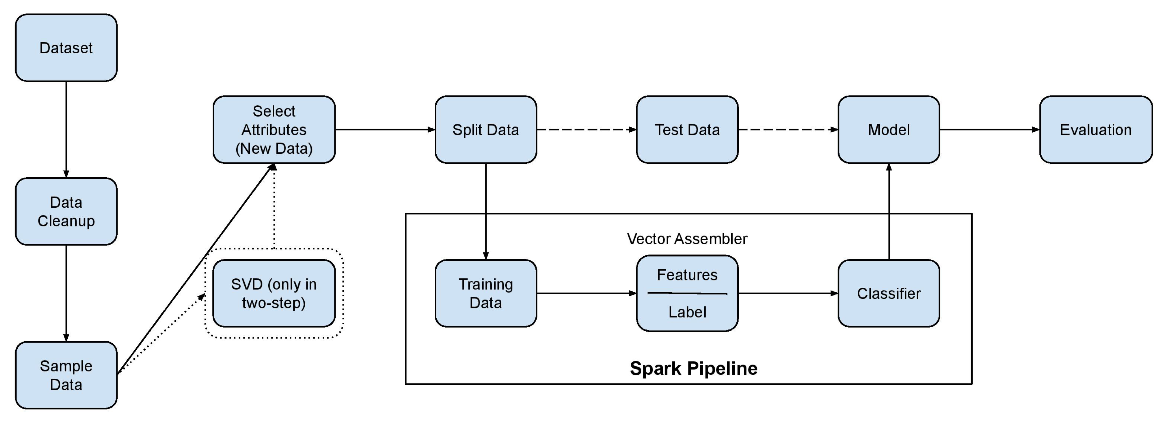
• SVD has been initially applied to the original data matrix in order to obtain a low dimensional representation with a smaller attribute set.
• The classifier has been subsequently applied to the new attribute set in order to obtain the final labellings.

In order to test our approach, we examined two different datasets, one binary and one multiclass, and we recorded the performance of various classification algorithms in a distributed environment. Each classification method had strengths and limitations, depending on the dataset. For example, in Higgs dataset, decision tree was mediocre, but in PAMAP, it outperformed all the other classification methods.

From this work, certain conclusions can be drawn. First and foremost, it shows the potential of Spark to apply well-known ML operations to big data seamlessly without knowing how the dataset is distributed across HDFS. Additionally, it should be noted that it is not always apparent how an ML algorithm, especially an iterative one, can be implemented in the Spark DAG paradigm. The latter demonstrates the important contribution of MLlib as it provides a number of important classification algorithms. Third, from an algorithmic perspective it shows that modular architectures based on preprocessing can be more efficient, especially in a distributed environment, and thus the computational resources given to the preprocessing step are well spent. This is especially true for the SVD, which is typically considered expensive in traditional computing systems for large datasets. Fourth, sophisticated algorithms add significantly to the performance of a system. The wallclock time required to complete classification has been used as the complexity benchmark for reasons stated in Section 4.

As for future work, more datasets can serve as performance benchmarks of the proposed classification method. More tests will yield a better understanding of the optimal combinations of feature set size and classifier. Of course, the cluster on which we run the classification methods is another key aspect of the cloud computing in general, so checking the same or similar algorithms and dataset on different clusters may prove fundamental and reveal latent knowledge.

Reference

References

1. Alexopoulos, A.; Kanavos, A.; Giotopoulos, K.C.; Mohasseb, A.; Bader-El-Den, M.; Tsakalidis, A.K. Incremental Learning for Large Scale Classification Systems. In IFIP International Conference on Artificial Intelligence Applications and Innovations; Iliadis, L., Maglogiannis, I., Plagianakos, V., Eds.; Springer: Cham, Switzerland, 2018; Volume 520, pp. 112–122. [Google Scholar]
2. Hand, D.J.; Mannila, H.; Smyth, P. Principles of Data Mining; MIT Press: Cambridge, MA, USA, 2001. [Google Scholar]
3. Fayyad, U.M.; Piatetsky-Shapiro, G.; Smyth, P. From Data Mining to Knowledge Discovery in Databases. AI Mag. 1996, 17, 37–54. [Google Scholar]
4. Witten, I.H.; Eibe, F.; Hall, M.A.; Pal, C.J. Data Mining: Practical Machine Learning Tools and Techniques, 3rd ed.; Morgan Kaufmann: Burlington, MA, USA, 2016. [Google Scholar]
5. Candes, E.; Tao, T. The Dantzig Selector: Statistical Estimation when p is Much Larger than n. Ann. Stat. 2007, 35, 2313–2351. [Google Scholar] [CrossRef] [Green Version]
6. Koltchinskii, V. The Dantzig Selector and Sparsity Oracle Inequalities. Bernoulli 2009, 15, 799–828. [Google Scholar] [CrossRef]
7. Koperski, K.; Han, J.; Stefanovic, N. An Efficient Two-Step Method for Classification of Spatial Data. In Proceedings of the International Symposium on Spatial Data Handling (SDH), Vancouver, BC, Canada, 11–15 July 1998; pp. 45–54. [Google Scholar]
8. Christen, P. A Two-Step Classification Approach to Unsupervised Record Linkage. In Proceedings of the 6th Australasian Data Mining Conference (AusDM), Gold Coast, Australia, 3–4 December 2007; pp. 111–119. [Google Scholar]
9. Lian, C.; Ruan, S.; Denoeux, T. An Evidential Classifier based on Feature Selection and Two-Step Classification Strategy. Pattern Recogn. 2015, 48, 2318–2327. [Google Scholar] [CrossRef] [Green Version]
10. Drakopoulos, G.; Stathopoulou, F.; Kanavos, A.; Paraskevas, M.; Tzimas, G.; Mylonas, P.; Iliadis, L. A Genetic Algorithm for Spatiosocial Tensor Clustering: Exploiting TensorFlow Potential; Springer: Berlin, Germany, 2019; pp. 1–11. [Google Scholar]
11. Alloghani, M.; Al-Jumeily, D.; Hussain, A.; Mustafina, J.; Baker, T.; Aljaaf, A.J. Implementation of Machine Learning and Data Mining to Improve Cybersecurity and Limit Vulnerabilities to Cyber Attacks. In Nature-Inspired Computation in Data Mining and Machine Learning; Yang, X.S., He, X.S., Eds.; Springer: Cham, Switzerland, 2020; Volume 855, pp. 47–76. [Google Scholar]
12. Alloghani, M.; Baker, T.; Al-Jumeily, D.; Hussain, A.; Mustafina, J.; Aljaaf, A.J. Prospects of Machine and Deep Learning in Analysis of Vital Signs for the Improvement of Healthcare Services. In Nature-Inspired Computation in Data Mining and Machine Learning; Yang, X.S., He, X.S., Eds.; Springer: Cham, Switzerland, 2020; Volume 855, pp. 113–136. [Google Scholar]
13. Moniruzzaman, A.B.M.; Hossain, S.A. NoSQL Database: New Era of Databases for Big data Analytics - Classification, Characteristics and Comparison. 2013. Available online: http://article.nadiapub.com/IJDTA/vol6_no4/1.pdf (accessed on 22 March 2020).
14. Melnik, S.; Gubarev, A.; Long, J.J.; Romer, G.; Shivakumar, S.; Tolton, M.; Vassilakis, T. Dremel: Interactive Analysis of Web-Scale Datasets. Proc. VLDB Endow. 2010, 3, 330–339. [Google Scholar] [CrossRef]
15. Malewicz, G.; Austern, M.H.; Bik, A.J.C.; Dehnert, J.C.; Horn, I.; Leiser, N.; Czajkowski, G. Pregel: A system for large-scale graph processing. In Proceedings of the ACM International Conference on Management of Data (SIGMOD), Indianapolis, IN, USA, 6–11 June 2010; pp. 135–146. [Google Scholar]
16. Isard, M.; Budiu, M.; Yu, Y.; Birrell, A.; Fetterly, D. Dryad: Distributed Data-Parallel Programs from Sequential. Building Blocks. In Proceedings of the 2nd ACM SIGOPS/EuroSys European Conference on Computer Systems, New York, NA, USA, 21 March 2007; pp. 59–72. [Google Scholar]
17. Low, Y.; Gonzalez, J.; Kyrola, A.; Bickson, D.; Guestrin, C.; Hellerstein, J.M. Distributed GraphLab: A Framework for Machine Learning in the Cloud. 2012. Available online: http://vldb.org/pvldb/vol5/p716_yuchenglow_vldb2012.pdf (accessed on 22 March 2020).
18. Zaharia, M.; Xin, R.S.; Wendell, P.; Das, T.; Armbrust, M.; Dave, A.; Meng, X.; Rosen, J.; Venkataraman, S.; Franklin, M.J.; et al. Apache Spark: A Unified Engine for Big Data Processing. Comm. ACM 2016, 59, 56–65. [Google Scholar] [CrossRef]
19. Shvachko, K.; Kuang, H.; Radia, S.; Chansler, R. The Hadoop Distributed File System. In Proceedings of the IEEE 26th Symposium on Mass Storage Systems and Technologies (MSST), Incline Village, NV, USA, 3–7 May 2010; pp. 1–10. [Google Scholar]
20. Dean, J.; Ghemawat, S. MapReduce: Simplified Data Processing on Large Clusters. Comm. ACM 2008, 51, 107–113. [Google Scholar] [CrossRef]
21. Shi, J.; Qiu, Y.; Minhas, U.F.; Jiao, L.; Wang, C.; Reinwald, B.; Özcan, F. Clash of the Titans: MapReduce vs. Spark for Large Scale Data Analytics. Proc. VLDB Endow. 2015, 8, 2110–2121. [Google Scholar] [CrossRef] [Green Version]
22. Koliopoulos, A.; Yiapanis, P.; Tekiner, F.; Nenadic, G.; Keane, J.A. A Parallel Distributed Weka Framework for Big Data Mining Using Spark. In Proceedings of the IEEE International Congress on Big Data, New York, NY, USA, 27 June–2 July 2015; pp. 9–16. [Google Scholar]
23. Hall, M.A.; Frank, E.; Holmes, G.; Pfahringer, B.; Reutemann, P.; Witten, I.H. The WEKA Data Mining Software: An Update. SIGKDD Explor. 2009, 11, 10–18. [Google Scholar] [CrossRef]
24. Yang, L.; Shi, Z. An Efficient Data Mining Framework on Hadoop using Java Persistence API. In Proceedings of the 10th IEEE International Conference on Computer and Information Technology (CIT), Bradford, UK, 29 June–1 July 2010; pp. 203–209. [Google Scholar]
25. Zhao, W.; Ma, H.; He, Q. Parallel K-Means Clustering Based on MapReduce; Springer: Berlin, Germany, 1 December 2009; pp. 674–679. [Google Scholar]
26. Kang, U.; Faloutsos, C. Big Graph Mining: Algorithms and Discoveries. SIGKDD Explor. 2012, 14, 29–36. [Google Scholar] [CrossRef]
27. Abadi, M.; Barham, P.; Chen, J.; Chen, Z.; Davis, A.; Dean, J.; Devin, M.; Ghemawat, S.; Irving, G.; Isard, M.; et al. TensorFlow: A system for large-scale machine learning. In Proceedings of the 12th USENIX Symposium on Operating Systems Design and Implementation (OSDI 16), Savannah, GA, USA, 2–4 November 2016; pp. 265–283. [Google Scholar]
28. Kyriazidou, I.; Drakopoulos, G.; Kanavos, A.; Makris, C.; Mylonas, P. Towards Predicting Mentions to Verified Twitter Accounts: Building Prediction Models over MongoDB with Keras. 2019. Available online: https://www.researchgate.net/profile/Georgios_Drakopoulos/publication/334681267_Towards_Predicting_Mentions_To_Verified_Twitter_Accounts_Building_Prediction_Models_Over_MongoDB_With_Keras/links/5d39dfe792851cd046869a4c/Towards-Predicting-Mentions-To-Verified-Twitter-Accounts-Building-Prediction-Models-Over-MongoDB-With-Keras.pdf (accessed on 22 March 2020).
29. Zhang, T. Solving Large Scale Linear Prediction Problems Using Stochastic Gradient Descent Algorithms. In Proceedings of the 21st International Conference on Machine Learning (ICML), Banff, AB, Canada, 4 July 2004. [Google Scholar]
30. Younis, O.; Fahmy, S. Distributed Clustering in Ad-hoc Sensor Networks: A Hybrid, Energy-Efficient Approach. In Proceedings of the 23rd Annual Joint Conference of the IEEE Computer and Communications Societies (INFOCOM), Hong Kong, China, 7–11 March 2004. [Google Scholar]
31. Januzaj, E.; Kriegel, H.; Pfeifle, M. DBDC: Density Based Distributed Clustering. In Advances in Database Technology - EDBT 2004; Bertino, E., Ed.; Springer: Berlin, Germany, 2004; Volume 2992, pp. 88–105. [Google Scholar]
32. Gorodetsky, V.; Karsaev, O.; Samoilov, V. Multi-agent Technology for Distributed Data Mining and Classification. In Proceedings of the IEEE/WIC International Conference on Intelligent Agent Technology (IAT), Halifax, NS, Canada, 13–17 October 2003; pp. 438–441. [Google Scholar]
33. Ghasemzadeh, H.; Loseu, V.; Jafari, R. Structural Action Recognition in Body Sensor Networks: Distributed Classification Based on String Matching. IEEE Trans. Inform. Tech. Biomed. 2010, 14, 425–435. [Google Scholar] [CrossRef] [PubMed]
34. Kokiopoulou, E.; Frossard, P. Distributed Classification of Multiple Observation Sets by Consensus. IEEE Trans. Signal Process. 2011, 59, 104–114. [Google Scholar] [CrossRef]
35. D’Costa, A.; Sayeed, A.M. Collaborative Signal Processing for Distributed Classification in Sensor Networks. In Information Processing in Sensor Networks; Zhao, F., Guibas, L., Eds.; Springer: Berlin, Germany, 2003; Volume 2634, pp. 193–208. [Google Scholar]
36. Malhotra, B.; Nikolaidis, I.; Harms, J.J. Distributed Classification of Acoustic Targets in Wireless audio-sensor Networks. Comput. Netw. 2008, 52, 2582–2593. [Google Scholar] [CrossRef]
37. Raychaudhuri, S. Introduction to Monte Carlo simulation. In Proceedings of the Winter Simulation Conference, Miami, FL, USA, 7–10 December 2008; pp. 91–100. [Google Scholar]
38. Meng, X.; Bradley, J.K.; Yavuz, B.; Sparks, E.R.; Venkataraman, S.; Liu, D.; Freeman, J.; Tsai, D.B.; Amde, M.; Owen, S.; et al. MLlib: Machine Learning in Apache Spark. J. Mach. Learn. Res. 2016, 17, 1235–1241. [Google Scholar]
39. Baltas, A.; Kanavos, A.; Tsakalidis, A. An Apache Spark Implementation for Sentiment Analysis on Twitter Data. In Algorithmic Aspects of Cloud Computing; Sellis, T., Oikonomou, K., Eds.; Springer: Cham, Switzerland, 2016; Volume 10230, pp. 15–25. [Google Scholar]
40. Sioutas, S.; Mylonas, P.; Panaretos, A.; Gerolymatos, P.; Vogiatzis, D.; Karavaras, E.; Spitieris, T.; Kanavos, A. Survey of Machine Learning Algorithms on Spark Over DHT-based Structures. In Algorithmic Aspects of Cloud Computing; Sellis, T., Oikonomou, K., Eds.; Springer: Cham, Switzerland, 2016; Volume 10230, pp. 146–156. [Google Scholar]
41. Kanavos, A.; Nodarakis, N.; Sioutas, S.; Tsakalidis, A.; Tsolis, D.; Tzimas, G. Large Scale Implementations for Twitter Sentiment Classification. Algorithms 2017, 10, 33. [Google Scholar] [CrossRef]
42. Kotsiantis, S.B. Supervised Machine Learning: A Review of Classification Techniques. Inform. (Slovenia) 2007, 31, 249–268. [Google Scholar]
43. Breiman, L. Random Forests. Mach. Learn. 2001, 45, 5–32. [Google Scholar] [CrossRef] [Green Version]
44. Mohan, A.; Chen, Z.; Weinberger, K.Q. Web-Search Ranking with Initialized Gradient Boosted Regression Trees. 2011. Available online: http://proceedings.mlr.press/v14/mohan11a/mohan11a.pdf (accessed on 22 March 2020).
45. Baldi, P.; Sadowski, P.; Whiteson, D. Searching for Exotic Particles in High-energy Physics with Deep Learning. Nat. Comm. 2014, 5, 4308. [Google Scholar] [CrossRef] [PubMed] [Green Version]
46. Reiss, A.; Stricker, D. Introducing a New Benchmarked Dataset for Activity Monitoring. In Proceedings of the International Symposium on Wearable Computers (ISWC), Newcastle, UK, 18–22 June 2012; pp. 108–109. [Google Scholar]
Figure 1. Knowledge discovery pipeline.
Algorithms 13 00071 g001
Figure 2. Proposed system architecture.
Algorithms 13 00071 g002
Figure 3. Apache Spark API stack.
Algorithms 13 00071 g003