p-Refined Multilevel Quasi-Monte Carlo for Galerkin Finite Element Methods with Applications in Civil Engineering

Abstract

Civil engineering applications are often characterized by a large uncertainty on the material parameters. Discretization of the underlying equations is typically done by means of the Galerkin Finite Element method. The uncertain material parameter can be expressed as a random field represented by, for example, a Karhunen–Loève expansion. Computation of the stochastic responses, i.e., the expected value and variance of a chosen quantity of interest, remains very costly, even when state-of-the-art Multilevel Monte Carlo (MLMC) is used. A significant cost reduction can be achieved by using a recently developed multilevel method: p-refined Multilevel Quasi-Monte Carlo (p-MLQMC). This method is based on the idea of variance reduction by employing a hierarchical discretization of the problem based on a p-refinement scheme. It is combined with a rank-1 Quasi-Monte Carlo (QMC) lattice rule, which yields faster convergence compared to the use of random Monte Carlo points. In this work, we developed algorithms for the p-MLQMC method for two dimensional problems. The p-MLQMC method is first benchmarked on an academic beam problem. Finally, we use our algorithm for the assessment of the stability of slopes, a problem that arises in geotechnical engineering, and typically suffers from large parameter uncertainty. For both considered problems, we observe a very significant reduction in the amount of computational work with respect to MLMC.

1. Introduction

There is an increasing need to accurately simulate and compute solutions to engineering problems, whilst accounting for model uncertainties. Methods for uncertainty quantification and propagation in engineering disciplines can be categorized into two groups: non-sampling and sampling methods.

Examples of non-sampling methods are the perturbation method and the Stochastic Galerkin Finite Element method. The perturbation method is based on a Taylor series expansion approximating the mean and variance of the solution [1]. While quite effective, its use is restricted to models with a limited number of relatively small uncertainties. The Stochastic Galerkin method, proposed by Ghanem and Spanos [2], is based on a spectral representation in the stochastic space. It transforms the uncertain coefficient partial differential equation (PDE) problem by means of a Galerkin projection technique into a large coupled system of deterministic PDEs. This method allows for somewhat larger numbers of uncertainties and is quite accurate. However, it is highly intrusive and memory demanding, making its implementation cumbersome, and restricting its use to still rather low stochastic dimensions.

Sampling methods, on the other hand, are typically non-intrusive. Each sample corresponds to a deterministic solve, with a particular choice for the parameter values. Two popular examples are the Stochastic Collocation method, see [3], and the Monte Carlo (MC) method, see [4]. The former samples a stochastic PDE at a carefully selected multidimensional set of collocation points. After this sampling, a Lagrange interpolation is performed, leading to a polynomial response surface. From this response surface, the relevant stochastic characteristics can easily be computed in a post-processing step. Like Stochastic Galerkin, the Stochastic Collocation method suffers from the curse of dimensionality: the computational cost grows exponentially with the number of random variables considered in the problem. The MC method on the other hand, selects its samples randomly and does not suffer from the curse of dimensionality. However, a drawback is its slow convergence as a function of the number of samples taken.

The convergence of Monte Carlo can be accelerated in a variety of ways. For example, an alternative non-random selection of sampling points can be used, as in Quasi-Monte Carlo [5,6] and Latin Hypercube [7] sampling methods. Other techniques, such as Multilevel Monte Carlo (MLMC) [8], Multilevel Quasi-Monte Carlo (MLQMC) [9] and its generalizations, see, e.g., [10,11], can speed up the method. These improved Monte Carlo methods are based on a hierarchy of meshes with increasing resolution, where samples on coarser meshes are computationally less expensive than samples on finer meshes.

For completeness, we mention that there also exist hybrid variants which exhibit both a sampling and non-sampling character. This type of methods combine, for example, the Stochastic Finite Element methodology with Monte Carlo sampling or a multi-dimensional cubature method, see, e.g., [12,13].

In previous work, we presented a comparison between Monte Carlo and Multilevel Monte Carlo [14], and between Multilevel Monte Carlo and Multilevel Quasi-Monte Carlo [15]. In this work, we will present a novel multilevel method: p-refined Multilevel Quasi-Monte Carlo (p-MLQMC). This method reduces the cost of the simulation by taking samples on a hierarchy of nested p-refined meshes, and by selecting the sample points in a non-random way.

In [16], the authors introduced a multi-order Monte Carlo algorithm (MOMC) for computing the statistics of quantities of interest described by linear hyperbolic equations with stochastic parameters. The MOMC method relies on a hierarchy of p-refined meshes, similar to the setup in this paper. A numerical analysis of MOMC, including numerical results for dispersion in long-distance propagation of waves subjected to uncertainty can be found in [16]. Our p-MLQMC method is also based on a hierarchy of p-refined meshes with the addition of a deterministic sampling rule. Our focus lies on the implementation and on the practicalities of p-MLQMC. We discuss how the uncertainty represented as a random field needs to be taken into account in the discretized versions of our civil/geotechnical model problem so as to ensure a minimal total computational cost. The MOMC method has a computational cost increase in function of a user requested tolerance $ϵ$, proportional to ${ϵ}^{-2}$, while for p-MLQMC this is close to ${ϵ}^{-1}$, because of the use of a deterministic sampling rule.

First we will introduce the multilevel methods and detail the technicalities pertaining to p-MLQMC. Here, we also discuss how the uncertainty is modeled and incorporated in our models. Second, we will present the two model problems on which we will test and benchmark our method. The model problems consist of an academic beam bending problem and a more complicated slope stability problem. Last, we present our results obtained with p-MLQMC.

2. p-Refined Multilevel Quasi-Monte Carlo

The Multilevel Monte Carlo method and Multilevel Quasi-Monte Carlo method are extensions of the standard Monte Carlo method, see, e.g., [8,9,17]. These methods rely on a clever combination of many computationally cheap low resolution samples and a relatively small number of higher resolution, but computationally more expensive samples. MLMC and MLQMC require a predefined hierarchy of meshes in order to work properly. Classically, the hierarchy of the meshes is based on a successive spatial refinement of the mesh per level, known as h-refinement. Hence, we will refer to classical MLMC and MLQMC as h-ML(Q)MC. Our p-MLQMC method, based on the MLQMC method, uses a spatial mesh refinement based on increasing the element’s polynomial order, i.e., p-refinement. In this section we will first give an overview of the main characteristics of the MLMC method, whereafter we give an overview of the MLQMC method, and highlight the differences with respect to the MLMC method. We then give an account of the mesh hierarchies before introducing the p-MLQMC algorithm. We conclude with a general complexity theorem for ML(Q)MC sampling.

2.1. The Multilevel and Multilevel Quasi Monte Carlo Methods

Let $\mathbb{E}\left[P_L\left({\mathbf{x}}^{\left(n\right)}\right)\right]$, or $\mathbb{E}\left[P_L\right]$ for short, be the expected value of a particular quantity of interest P depending on a set of random variables ${\mathbf{x}}_L^{\left(n\right)}$, discretized on mesh L. The standard MC estimator for $\mathbb{E}\left[P_L\right]$ using $N_L$ samples on mesh L, denoted as $Q_L^{\mathrm{MC}}$, can be written as

$$Q_L^{\mathrm{MC}}:=\frac{1}{N_L}\sum _{n=1}^{N_L}{P}_L\left({\mathbf{x}}_L^{\left(n\right)}\right).$$

(1)

The MLMC method, on the other hand, starts from a reformulation of $\mathbb{E}\left[P_L\right]$ as a telescoping sum. The expected value of the quantity of interest on the finest mesh L is expressed as the expected value of the quantity of interest on the coarsest mesh, plus a series of correction terms (or differences), i.e.,

$$\mathbb{E}\left[P_L\right]=\mathbb{E}\left[P_0\right]+\sum _{\ell =1}^L\mathbb{E}[P_{\ell }-P_{\ell -1}]=\sum _{\ell =0}^L\mathbb{E}\left[\Delta P_{\ell }\right],$$

(2)

where we defined $\Delta P_{\ell }:=P_{\ell }\left({\mathbf{x}}_{\ell }\right)-P_{\ell -1}\left({\mathbf{x}}_{\ell }\right)$ with $P_{-1}:=0$.

Each term on the right-hand side is then estimated separately by a standard MC estimator with $N_{\ell }$ samples, i.e.,

$$Q_L^{\mathrm{MLMC}}:=\frac{1}{N_0}\sum _{n=1}^{N_0}{P}_0\left({\mathbf{x}}_0^{\left(n\right)}\right)+\sum _{\ell =1}^L\left\{\frac{1}{N_{\ell }}\sum _{n=1}^{N_{\ell }}\left(P_{\ell }\left({\mathbf{x}}_{\ell }^{\left(n\right)}\right)-P_{\ell -1}\left({\mathbf{x}}_{\ell }^{\left(n\right)}\right)\right)\right\},$$

(3)

where $Q_L^{\mathrm{MLMC}}$ is the MLMC estimator for the expected value $\mathbb{E}\left[P_L\right]$, which is a discrete approximation for the expected value of the quantity of interest, $\mathbb{E}\left[P\right]$. The MLMC estimator in Equation (3) can be written as a sum of $L+1$ estimators for the expected value of the difference on each level, i.e.,

$$Q_L^{\mathrm{MLMC}}=\sum _{\ell =0}^L\frac{1}{N_{\ell }}\sum _{n=1}^{N_{\ell }}\Delta P_{\ell }^{\left(n\right)},$$

(4)

where we defined $\Delta P_{\ell }^{\left(n\right)}:=P_{\ell }({\mathbf{x}}_{\ell }^{\left(n\right)})-P_{\ell -1}({\mathbf{x}}_{\ell }^{\left(n\right)})$ with $P_{-1}^{\left(n\right)}:=0$.

Because of the telescoping sum property, i.e., Equation (2), the MLMC estimator is an unbiased estimator for the quantity of interest on the finest mesh, i.e.,

$$\mathbb{E}\left[Q_L^{\mathrm{MLMC}}\right]=\mathbb{E}\left[P_L\right].$$

(5)

The error is controlled by imposing a tolerance ${ϵ}^2$ on the mean square error (MSE) of the estimator, defined as

$$\begin{array}{cc}\hfill \mathrm{MSE}\left(Q_L^{\mathrm{MLMC}}\right)& :=\mathbb{E}\left[{\left(Q_L^{\mathrm{MLMC}}-\mathbb{E}\left[P\right]\right)}^2\right]\hfill \\ \hfill & =\mathbb{V}\left[Q_L^{\mathrm{MLMC}}\right]+{\left(\mathbb{E}\left[Q_L^{\mathrm{MLMC}}\right]-\mathbb{E}\left[P\right]\right)}^2\hfill \\ \hfill & =\mathbb{V}\left[Q_L^{\mathrm{MLMC}}\right]+{\left(\mathbb{E}\left[P_L-P\right]\right)}^2.\hfill \end{array}$$

(6)

The right-hand side of Equation (6) consists of two parts: the variance of the estimator, $\mathbb{V}\left[Q_L^{\mathrm{MLMC}}\right]$, and the squared bias, ${\left(\mathbb{E}\left[P_L-P\right]\right)}^2$. The stopping criterion for multilevel schemes is typically based on the requirements that both terms are less than ${ϵ}^2/2$. The root mean square error (RMSE) is defined as, $\mathrm{RMSE}\left(Q_L^{\mathrm{MLMC}}\right)=\sqrt{\mathrm{MSE}\left(Q_L^{\mathrm{MLMC}}\right)}$.

The variance of the estimator satisfies

$$\mathbb{V}\left[Q_L^{\mathrm{MLMC}}\right]=\sum _{\ell =0}^L\frac{V_{\ell }}{N_{\ell }},$$

(7)

with $V_{\ell }:=\mathbb{V}\left[\Delta P_{\ell }\right]$ the variance of the difference, which is used to determine the number of samples $N_{\ell }$ needed on each level ℓ. This is done by following the classic argument by Giles in [8], where the total cost of the MLMC estimator,

$$\cos \mathrm{t}\left(Q_L^{\mathrm{MLMC}}\right)=\sum _{\ell =0}^L{N}_{\ell }{C}_{\ell },$$

(8)

is minimized, with $C_{\ell }$ denoting the cost to compute a single realization of the difference $\Delta P_{\ell }^{\left(n\right)}$, subjected to the constraint

$$\sum _{\ell =0}^L\frac{V_{\ell }}{N_{\ell }}\le \frac{{ϵ}^2}{2}.$$

(9)

When treating the $N_{\ell }$ as continuous variables, one finds

$$N_{\ell }=\frac{2}{{ϵ}^2}\sqrt{\frac{V_{\ell }}{C_{\ell }}}\sum _{\ell =0}^L\sqrt{V_{\ell }{C}_{\ell }}.$$

(10)

The second term in Equation (6) is used to determine the maximum number of levels L. A typical MLMC implementation is level-adaptive, i.e., starting from a coarse finite element mesh, finer meshes are only added if required to reach a certain accuracy. Assuming that the convergence $\mathbb{E}\left[P_{\ell }\right]\to \mathbb{E}\left[P\right]$ is bounded as $|\mathbb{E}[P_{\ell }-P]|=\mathcal{O}\left(2^{-\alpha \ell }\right)$, then we can use the heuristic

$$|\mathbb{E}[P_L-P]|=\left|\sum _{\ell =L+1}^{\infty }\mathbb{E}[\Delta P_{\ell }]\right|\approx \frac{|\mathbb{E}[\Delta P_L]|}{2^{\alpha }-1}$$

(11)

and check for convergence using $|\mathbb{E}[P_L-P_{L-1}]|/(2^{\alpha }-1)\le ϵ/\sqrt{2}$, see [8] for details.

The MLQMC estimator has a similar formulation as MLMC. It differs in that it uses an average over a number of shifts $R_{\ell }$ on each level, and a set of deterministic sample points ${\mathbf{x}}_{\ell }^{(r,n)}$, i.e.,

$$Q_L^{\mathrm{MLQMC}}=\frac{1}{R_0}\sum _{r=1}^{R_0}\frac{1}{N_0}\sum _{n=1}^{N_0}{P}_0({\mathbf{x}}_0^{(r,n)})+\sum _{\ell =1}^L\frac{1}{R_{\ell }}\sum _{r=1}^{R_{\ell }}\left\{\frac{1}{N_{\ell }}\sum _{n=1}^{N_{\ell }}\left(P_{\ell }({\mathbf{x}}_{\ell }^{(r,n)})-P_{\ell -1}({\mathbf{x}}_{\ell }^{(r,n)})\right)\right\}.$$

(12)

This can again be rewritten as a sum of $L+1$ estimators, analogous as in Equation (4),

$$Q_L^{\mathrm{MLQMC}}=\sum _{\ell =0}^L\frac{1}{R_{\ell }}\sum _{r=1}^{R_{\ell }}\frac{1}{N_{\ell }}\sum _{n=1}^{N_{\ell }}\Delta P_{\ell }^{\left(r,n\right)},$$

(13)

where we defined $\Delta P_{\ell }^{\left(r,n\right)}:=P_{\ell }({\mathbf{x}}_{\ell }^{(r,n)})-P_{\ell -1}({\mathbf{x}}_{\ell }^{(r,n)})$ with $P_{-1}^{(r,n)}:=0$.

The major difference between MLMC and MLQMC is the choice of the sample points. For the MLMC estimator in Equation (3), the sample points ${\mathbf{x}}_{\ell }^{\left(n\right)}$ are chosen at random from a given distribution. For MLQMC however, the sample points ${\mathbf{x}}_{\ell }^{(r,n)}$ are optimally chosen in the stochastic space, based on a deterministic rule. Here, we use a rank-1 lattice rule, similar to [9]. By using these deterministic points, three practicalities must be addressed in order for MLQMC to work.

The first practicality pertains to the additional bias that is being generated on the stochastic quantities of the computed solution when using these deterministic points. In order to recover unbiased estimates, a number of random shifts ${\mathsf{\Xi }}_r,r=1,2,\dots ,R_{\ell }$ with ${\mathsf{\Xi }}_r\in {\left[0,1\right]}^s$, has to be introduced on each level. This leads to the extra summation in the MLQMC estimator in Equation (12), see Section 2.9 of [18].

The representation of the MLQMC sample points with inclusion of the aforementioned random shifts is as follows:

$${\mathbf{x}}^{\left(r,n\right)}=\mathrm{frac}\left(\frac{n}{N}\mathbf{z}+{\mathsf{\Xi }}_r\right)\mathrm{for}n=0,\dots ,N-1,$$

(14)

where $\mathrm{frac}\left(x\right)=x-x,x>0$, $\mathbf{z}$ is an s-dimensional vector of positive integers and N is the number of points in the lattice rule.

The second practicality relates to the number of points computed according to Equation (14). It is clear that the total number of points N needs to be known beforehand and thus cannot increase adaptively. Such a type of closed lattice rule cannot easily be used in an adaptive algorithm where additional samples are added on the fly. By rewriting Equation (14) as

$${\mathbf{x}}^{\left(r,n\right)}=\mathrm{frac}\left({\varphi }_2\left(n\right)\mathbf{z}+{\mathsf{\Xi }}_r\right)\mathrm{for}n\in \mathbb{N},$$

(15)

with ${\varphi }_2$ the radical inverse function in base 2, it is however possible to obtain an open lattice rule, i.e., removing the need to know N beforehand [19]. The radical inverse function in base 2 mirrors the binary representation of a number around its binary point ensuring that ${\varphi }_2\left(n\right)\in \left[0,1\right)$.

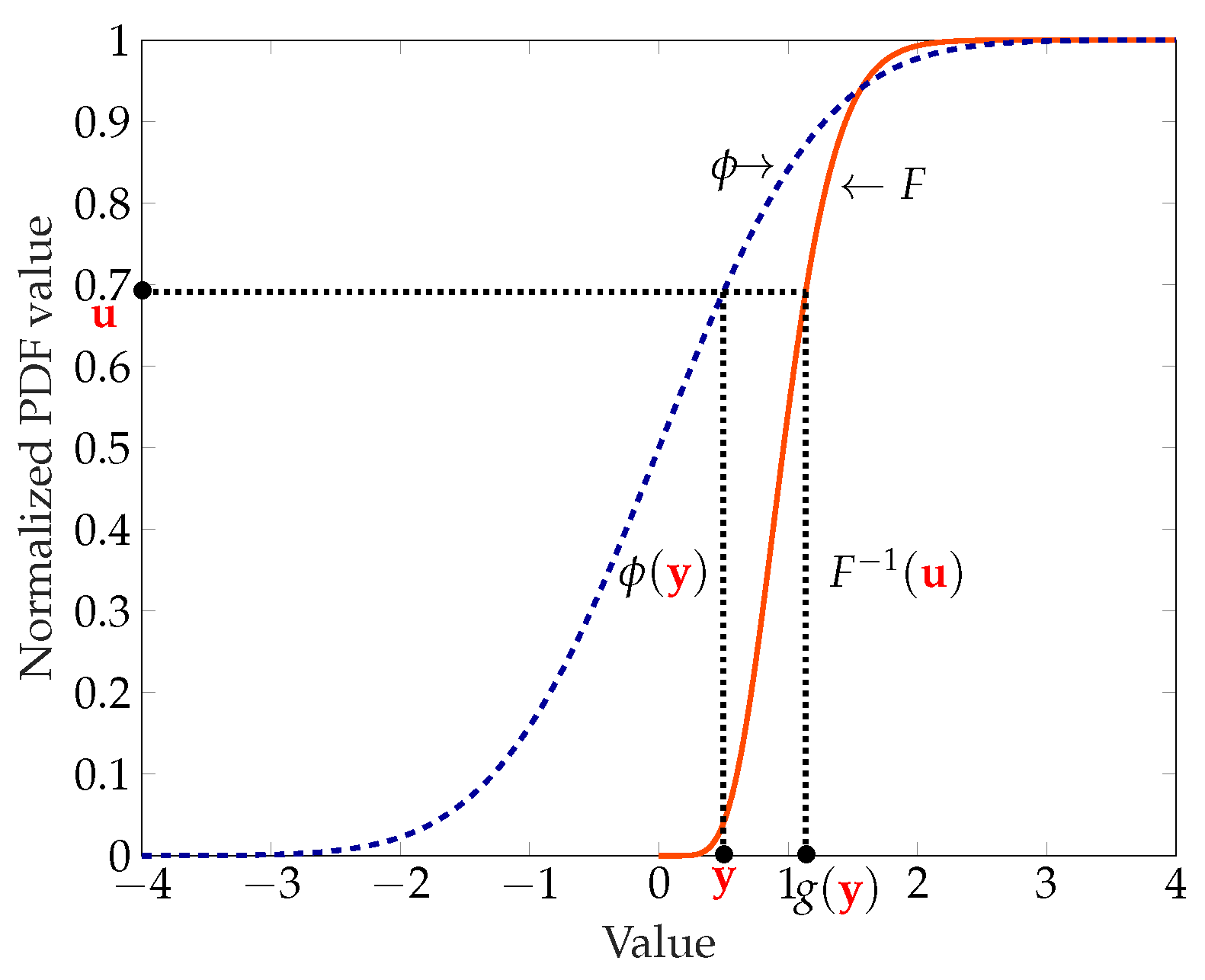
The third practicality concerns the computation of the points ${\mathbf{x}}^{(r,n)}$. These points are spatially located in the unit cube, that is ${\mathbf{x}}^{\left(r,n\right)}\in {\left[0,1\right)}^s$. In order to use these points in a Monte Carlo simulation that uses normally distributed random numbers, every set of points must be mapped from the ${[0,1)}^s$ to ${\mathbb{R}}^s$. For this the inverse, ${\mathsf{\Phi }}^{-1}$, of the univariate standard normal cumulative distribution function, $\mathsf{\Phi }\left(y\right)={\int }_{-\infty }^{y}exp\left(-t^2/2\right)/\sqrt{2\pi }dt$, is applied point wise to Equation (15), see [20]. This is written as

$${\mathbf{x}}^{\left(r,n\right)}={\mathsf{\Phi }}^{-1}\left(\mathrm{frac}\left({\varphi }_2\left(n\right)\mathbf{z}+{\mathsf{\Xi }}_r\right)\right)\mathrm{for}n\in \mathbb{N}.$$

(16)

The discussion pertaining to MLMC is applicable to MLQMC, with the exception of the part related to the computation of the number of samples. Unlike MLMC, the number of samples for MLQMC is not based on a formula as in Equation (10). In order to satisfy the statistical constraint, i.e., Equation (9), an adaptive algorithm is used, see [9]. Starting with an initial number of samples, this algorithm multiplies the number of samples on the level with maximum ratio ${\mathcal{V}}_{\ell }/C_{\ell },$ with a constant factor until the variance of the estimator $\mathbb{V}\left[Q_L^{\mathrm{MLQMC}}\right]={\sum }_{\ell =0}^L{\mathcal{V}}_{\ell }$ is smaller than ${ϵ}^2/2$. In our implementation this multiplication constant is chosen as $1.2$, and ${\mathcal{V}}_{\ell }$ is computed as

$${\mathcal{E}}_{\ell }:=\frac{1}{R_{\ell }}\sum _{r=1}^{R_{\ell }}\left\{\frac{1}{N_{\ell }}\sum _{n=1}^{N_{\ell }}\left(\Delta P_{\ell }^{\left(n,r\right)}\right)\right\},$$

(17)

and

$${\mathcal{V}}_{\ell }:=\frac{1}{R_{\ell }(R_{\ell }-1)}\sum _{r=1}^{R_{\ell }}\left\{{\left(\frac{1}{N_{\ell }}\sum _{n=1}^{N_{\ell }}\left(\Delta P_{\ell }^{\left(n,r\right)}\right)-{\mathcal{E}}_{\ell }\right)}^2\right\}.$$

(18)

The number of samples is multiplied by 1.2 (instead of the naive value 2) because, in the current setting where each sample involves the solution of a complex PDE, an exponential growth with a doubling of the number of samples is a dramatic event that causes huge jumps in the total cost of the estimator. Reducing this value from 2 to 1.2, as in, for example [21], is a compromise that causes a more gradual increase of the computational cost of the estimator, while, at the same time ensuring that enough progress is made. Note that increasing the amount of samples one at the time, i.e., the other extreme, would not be efficient in a parallel implementation, such as the one in this paper. We note that if the updated number of samples is not an integer, the least integer greater than this value is taken in order to have an integer value as updated number of samples.

In this work, we use a shifted rank-1 lattice rule in order to generate the MLQMC sample points ${\mathbf{x}}_{\ell }^{(r,n)}$, as is commonly done in other work regarding MLQMC, see for example [9,10,22]. Rank-1 lattice rules belong to one of two major classes of QMC points, i.e. lattices. The other class consists of digital nets/sequences, of which Sobol’ sequences are one of the oldest example, see [23]. One of the major differences between these two classes, is that rank-1 lattice rules rely on a generating vector $\mathbf{z}$ to construct the points, while digital nets/sequences rely on a set of generating matrices $C_1,\dots ,C_s$. The shifting procedure, also referred to as randomization, as done in Equation (14) for rank-1 lattice rules, also differs for both classes. Shifting in rank-1 lattice rules is mathematically easier than digital shifting or scrambling in digital nets/sequences. (Digital) shifting allows for a faster convergence rate compared to the standard Monte Carlo method if the function under consideration is sufficiently smooth. We note that scrambling, which is only applicable to digital nets/sequences, can further improve the QMC convergence rate. For a more thorough discussion on this subject, we refer to [18].

The generating vector $\mathbf{z}$ we use for p-MLQMC is available from [24]. This vector was constructed with the component-by-component (CBC) algorithm with decreasing weights, ${\gamma }_j=1/j^2$.

2.2. Mesh Hierarchies

Multilevel methods rely on a hierarchy of levels to achieve variance reduction and, by doing so, reduce the total computational cost. In common practice, this hierarchy of levels is defined as a hierarchy of successively refined nested grids or meshes with a discretization based on the Finite Element Galerkin approximation. For a bounded domain $\mathsf{\Omega }$ in ${\mathbb{R}}^2$, a mesh $\mathcal{T}$ on $\mathsf{\Omega }$ is a partition into a number $M\left(\mathcal{T}\right)$ of open disjoint subdomains $\mathcal{T}={\left\{T_j\right\}}_j^{M\left(\mathcal{T}\right)}$ with a mesh width h. We follow Ciarlet’s definition of a finite element defined as triples $\left(T,\mathcal{P},\mathcal{N}\right)$, see [25].

Definition 1.

A finite element is defined as $\left(T,\mathcal{P},\mathcal{N}\right)$ with

1. 

$T\subseteq \mathbb{R}$ a closed subset with nonempty interior and piecewise smooth boundary, i.e., the element domain,

2. 

$\mathcal{P}$ a finite-dimensional space of functions on T, i.e., the space of shape functions, and

3. 

$\mathcal{N}=\left(N_1,N_2,\dots ,N_k\right)$a basis for${\mathcal{P}}^{\prime }$, i.e., the set of nodal variables.

Classically, the mesh hierarchy used for MLMC and MLQMC is based on an h-refinement scheme, i.e., a succession of meshes ${\mathcal{T}}_0,{\mathcal{T}}_{\ell },\dots ,{\mathcal{T}}_L$ such that $h_0>h_{\ell }>\dots >h_L$ and $M\left({\mathcal{T}}_0\right)<M\left({\mathcal{T}}_{\ell }\right)<\dots <M\left({\mathcal{T}}_L\right)$. Figure 1 and Figure 2 show a hierarchy of nested uniform h-refined meshes, for the numerical examples considered in Section 3.1 and Section 3.3, where the nodal points are at the intersections of the line segments.

In the present paper, we propose to use a hierarchy of meshes based on a p-refinement scheme i.e., increasing the polynomial order of the interpolating shape functions, $\left(T,{\mathcal{P}}_1,{\mathcal{N}}_1\right)\in {\mathcal{T}}_0<\left(T,{\mathcal{P}}_{\ell +1},{\mathcal{N}}_{\ell +1}\right)\in {\mathcal{T}}_{\ell }<\dots <\left(T,{\mathcal{P}}_{L+1},{\mathcal{N}}_{L+1}\right)\in {\mathcal{T}}_L$, such that $dim{\mathcal{P}}_1<dim{\mathcal{P}}_{\ell +1}<\dots <dim{\mathcal{P}}_{L+1}$. Figure 3 and Figure 4 show a hierarchy of nested p-refined meshes, where the nodal points are represented as red dots.

In this paper we will only consider two-dimensional uniform, Lagrange type elements. In order to construct both mesh refinement hierarchies, we use a combination of the open source mesh generator Gmsh [26] and Matlab [27].

2.3. Algorithm

Algorithm 1 describes the implementation for p-MLQMC. The output produced by the algorithm consists of the expected value of the estimator for a given tolerance $ϵ$ on the root mean square error. The algorithm computes the expected value of the estimator and its variance on each level according to Equations (17) and (18). The algorithm starts with $R_{\ell }=10$ and $N_{\ell }=2$ on each level ℓ. The value of $R_{\ell }$ is typically chosen to be small, in the range of 10 to 32, in order to have a fair comparison with MLMC, see ([28], page 3678) and ([9], page 6). In Algorithm 1, the bias B is evaluated by Equation (11). The expected value $\mathbb{E}\left[Q_L^{\mathrm{MLQMC}}\right]={\sum }_{\ell =0}^L{\mathcal{E}}_{\ell }$, where ${\mathcal{E}}_{\ell }$ follows from Equation (17).

Algorithm 1: p-MLQMC.

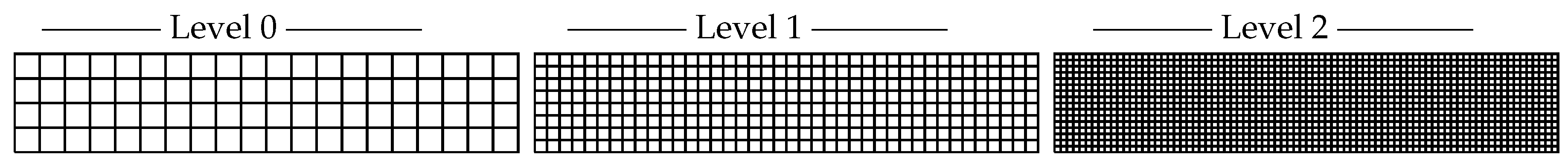
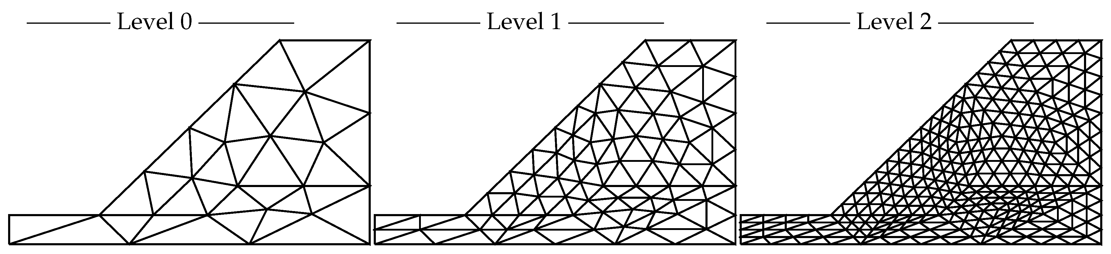
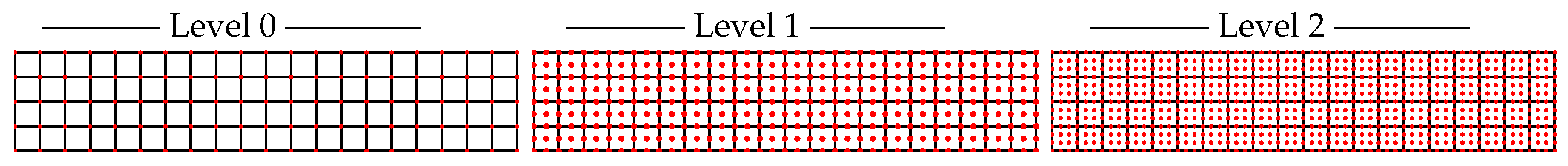
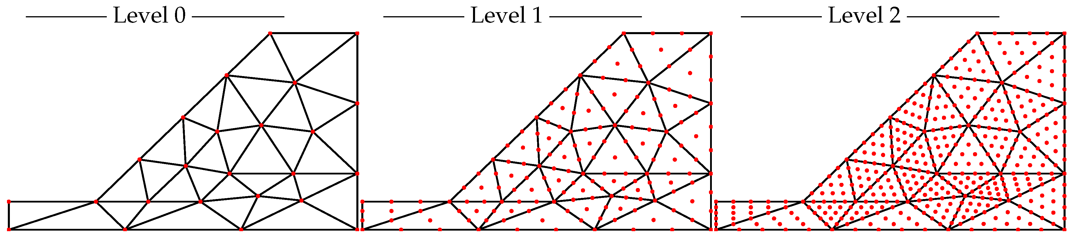
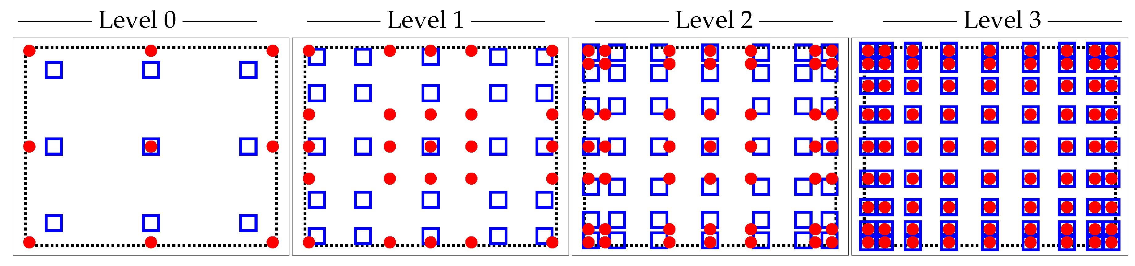
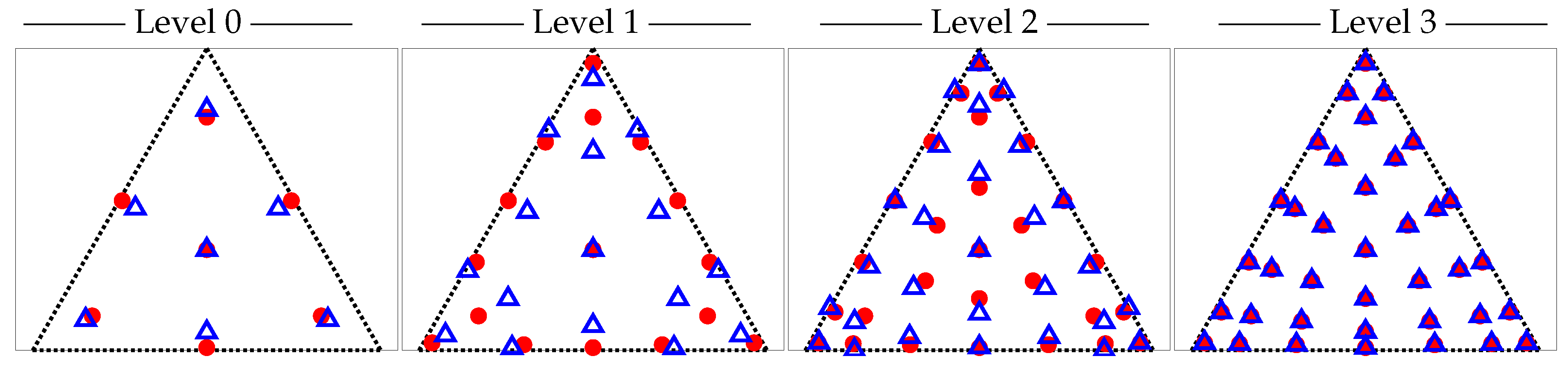
For this p-MLQMC algorithm to be able to work well, it is important to adequately generate the mesh hierarchy based on p-refinement. The challenge consists of selecting adequate points, on each level, in which to compute the discrete values of the random field. We generate these points starting from a given Gauss quadrature set on the finest level, i.e., level 3 for both our model problems. This is illustrated for one element for model problem 1 in Figure 5 and for model problem 2 in Figure 6. The ☐ and ∆, respectively represent the location of the actual Gauss quadrature points for a square and a triangular element, while the ● represent the location of the points where the values of the random field will be computed. This approach contrasts with a more intuitive one, which would consist of selecting the location of the actual Gauss quadrature points for the generation of the values of the random field. We observed numerically that our approach yields a larger decay of the expected value and variance of the multilevel differences compared to choosing the actual Gauss quadrature points for sampling from the random field, since, in that case the sets of quadrature points on different levels are not contained in each other, i.e., ☐₀ ⊈ ☐_ℓ ⊈ … ⊈ ☐_L. Such an inclusion property does hold however for our sets of random field evaluation points, i.e., ●₀ ⊆ ●_ℓ ⊆ … ⊆ ●_L. This implies that the sets of random values that are generated in these sets of points will also be included in one another. This will lead to a good decrease of $\mathbb{V}\left[\Delta P_{\ell }\right]$, as is required by the multilevel methodology. Note that on level 3, both ☐ and ∆ have the same spatial location as ●. We use the Gauss quadrature set on the finest mesh as a starting point for the construction of subsets on coarser meshes. The computed discrete random values are used during the numerical integration of the element stiffness matrix by means of Gauss quadrature points, see Section 2.6 for further details.

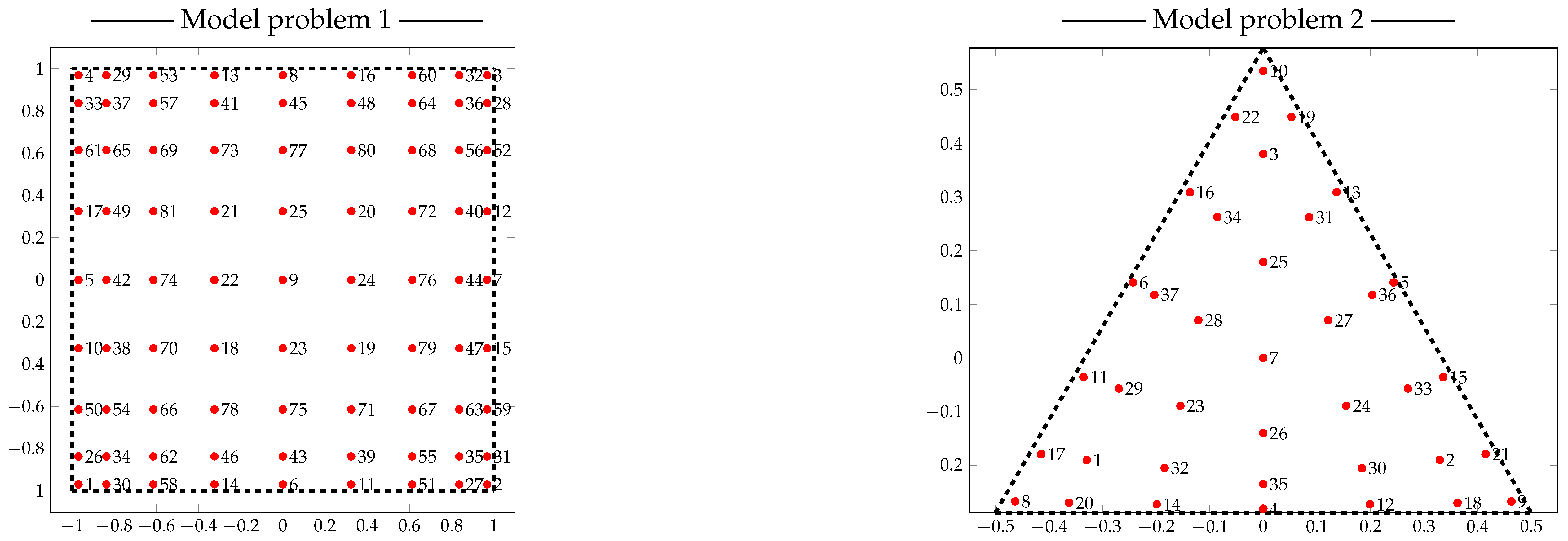
We will now describe an algorithm which generates the location of the points in which the discrete values of the random field are to be computed. Figure 5 and Figure 6, show the location of these points ●. As input to this algorithm, we require a set of Gauss quadrature points in natural coordinates for one element of the finest considered mesh. An algorithm for generating the point sets on each level is given in Algorithm 2. The output consists of a vector of points in which the discrete values of the random field are to be computed. This vector contains all the locations of the points on the finest level. Because the vector is sorted, taking subsets hereof gives the locations of the points on the coarser levels. Figure 7 shows in which sequence the points are chosen on a unit square and on a unit triangle. For example, for model problem 2, the evaluation points at the coarsest level are points $\left\{1,2,3,4,5,6,7\right\}$, the second coarsest level points $\left\{1,\dots ,7,8,9,10,11,12,13,14,15,16\right\}$, the third coarsest level points $\left\{1,\dots ,16,17,18,19,20,21,22,23,24,25,26,27,28\right\}$, and at the finest level points $\left\{1,\dots ,28,29,30,31,32,33,34,35,36,37\right\}$. See also

Table 1. Number of elements, degrees of freedom, element order and number of quadrature points for model problem 1.

	h-ML(Q)MC				p-ML(Q)MC
Level	Nel	DOF	Order	Nquad	Nel	DOF	Order	Nquad
0	80	210	1	9	80	210	1	9
1	320	738	1	9	80	738	2	25
2	1280	2754	1	9	80	1586	3	49
3	5120	10,626	1	9	80	2754	4	81
4	20,480	41,730	1	9	/	/	/	/

and

Table 2. Number of elements, degrees of freedom, element order and number of quadrature points for model problem 2.

	h-ML(Q)MC				p-ML(Q)MC
Level	Nel	DOF	Order	Nquad	Nel	DOF	Order	Nquad
0	33	48	1	7	33	48	1	7
1	132	160	1	7	33	338	3	16
2	528	582	1	7	33	892	5	28
3	2112	2218	1	7	33	1720	7	37
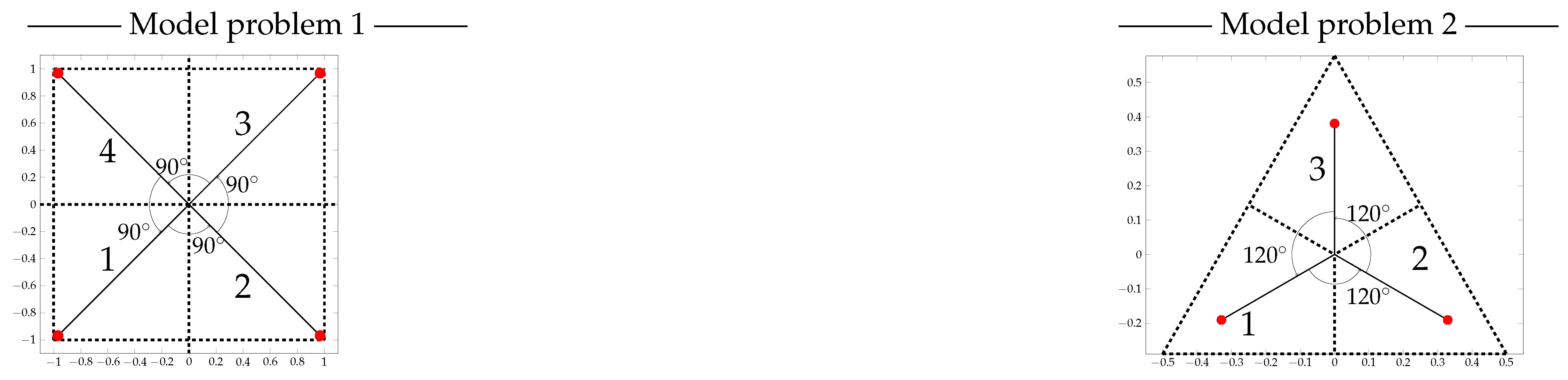
4	8448	8658	1	7	/	/	/	/

which, among other, list the number of quadrature points used per level. Once the locations of the points for one element in natural coordinates for each level have been obtained, the points are mapped to each element of the mesh by means of a transformation matrix. This results in a point set, listing the locations in global coordinates where the discrete values of the random field for the model problem are to be computed. As such, Algorithm 2 only works for two dimensional problems. Algorithm 2 consists of two main loops, the first loop starts on line 3, and returns a set of points which are closest to points of a given quadrature set on level ℓ. The second loop, starting on line 12, reorders the obtained set of closest points as in Figure 7, following the principle illustrated in Figure 8. Extending Algorithm 2 for three dimensions can be done be rewriting lines 12 to 24 to accommodate a reordering in three dimensions or to not consider a reordering at all. This would mean that lines 12 to 24 have to be omitted when computing the locations for the points in three dimensions.

Algorithm 2: Point Set Generation

In its current form, Algorithm 1 is level-adaptive, in the sense that levels are added to the estimator ($L\leftarrow L+1$) only when needed to reduce the bias. This means that the maximum level L that satisfies the bias constraint is not known a priori. The p-MLQMC method in Algorithm 1 takes as input a number of meshes ${\left\{{\mathcal{T}}_{\ell }\right\}}_{\ell =0\dots L}$ with maximum L, generated during a preprocessing step using the point selection method in Algorithm 2. If the bias constraint were not satisfied with the predefined maximum level L, it would force us to recompute a hierarchy of meshes ${\left\{{\mathcal{T}}_{\ell }\right\}}_{\ell =0\dots L}$ with a higher level L by means of Algorithm 2, and restart Algorithm 1 with these new meshes. The implication hereof is that samples from earlier runs of Algorithm 1 with maximum level L cannot be reused when restarting Algorithm 1 with maximum level $L+1$. The reason is that the inclusion principle is needed for the locations where discrete values of the random field are generated, as stated here above. In our implementation, we run Algorithm 2 only once for an a priori determined maximum level L, so that the set of points where the random field must be computed on each level remains the same during the course of Algorithm 1.

2.4. Cost Complexity Theorem

Having introduced the p-MLQMC method, we now present a complexity theorem for MLQMC, which also covers the MLMC method, when $\delta =1$. More details can be found in [22] and in ([29], page 76). We refer to [8] for the original MLMC complexity theorem and its generalization on which the current theorem is based, see [17].

Theorem 1.

Given the positive constants $\alpha ,\beta ,\gamma ,c_1,c_2,c_3$ such that $\alpha \ge {\displaystyle \frac{1}{2}}\min \left(\beta ,{\delta }^{-1}\gamma \right)$ with $\delta \in \left(1/2,1\right]$, and assume that the following conditions hold:

1. 

$\left|\mathbb{E}[P_{\ell }-P]\right|\le c_1{2}^{-\alpha \ell }$,

2. 

$\mathbb{V}\left[Q_{\ell }^{\mathrm{ML}\left(\mathrm{Q}\right)\mathrm{MC}}\right]\le c_2{2}^{-\beta \ell }{N}_{\ell }^{-1/\delta }$ and

3. 

$C_{\ell }\le c_3{2}^{\gamma \ell }$.

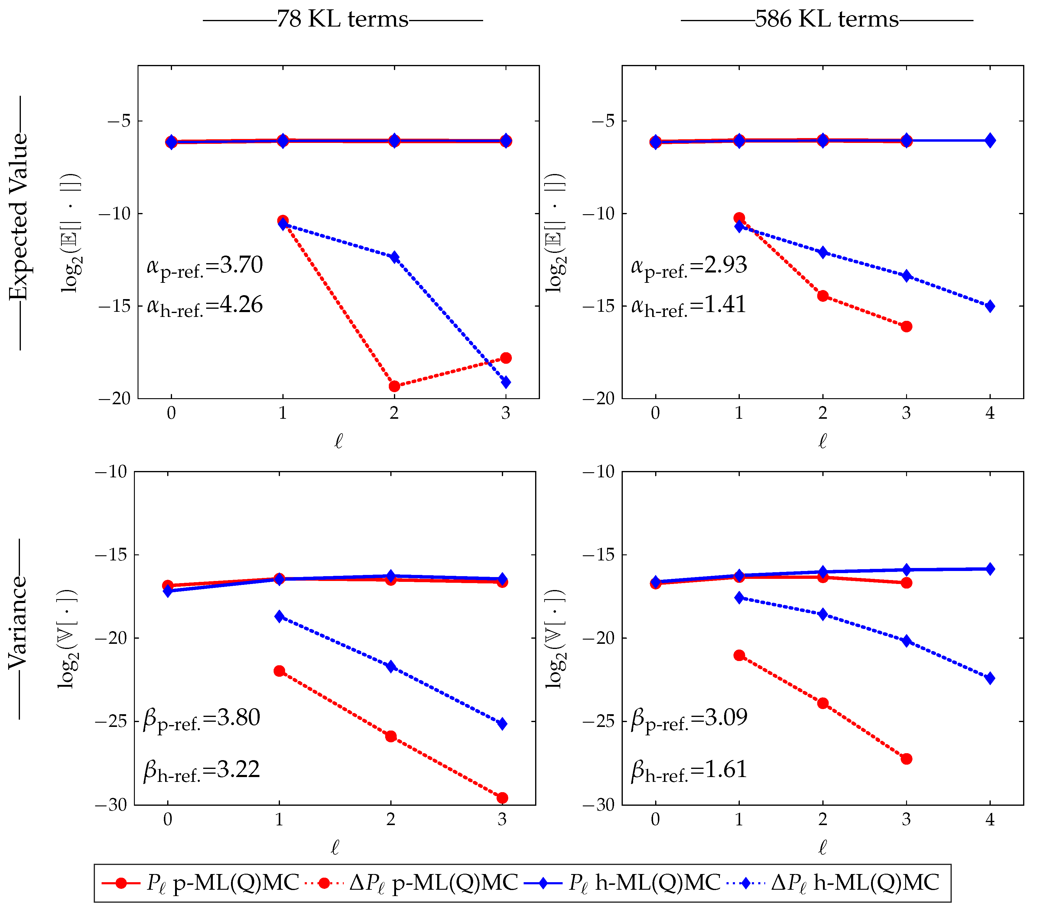
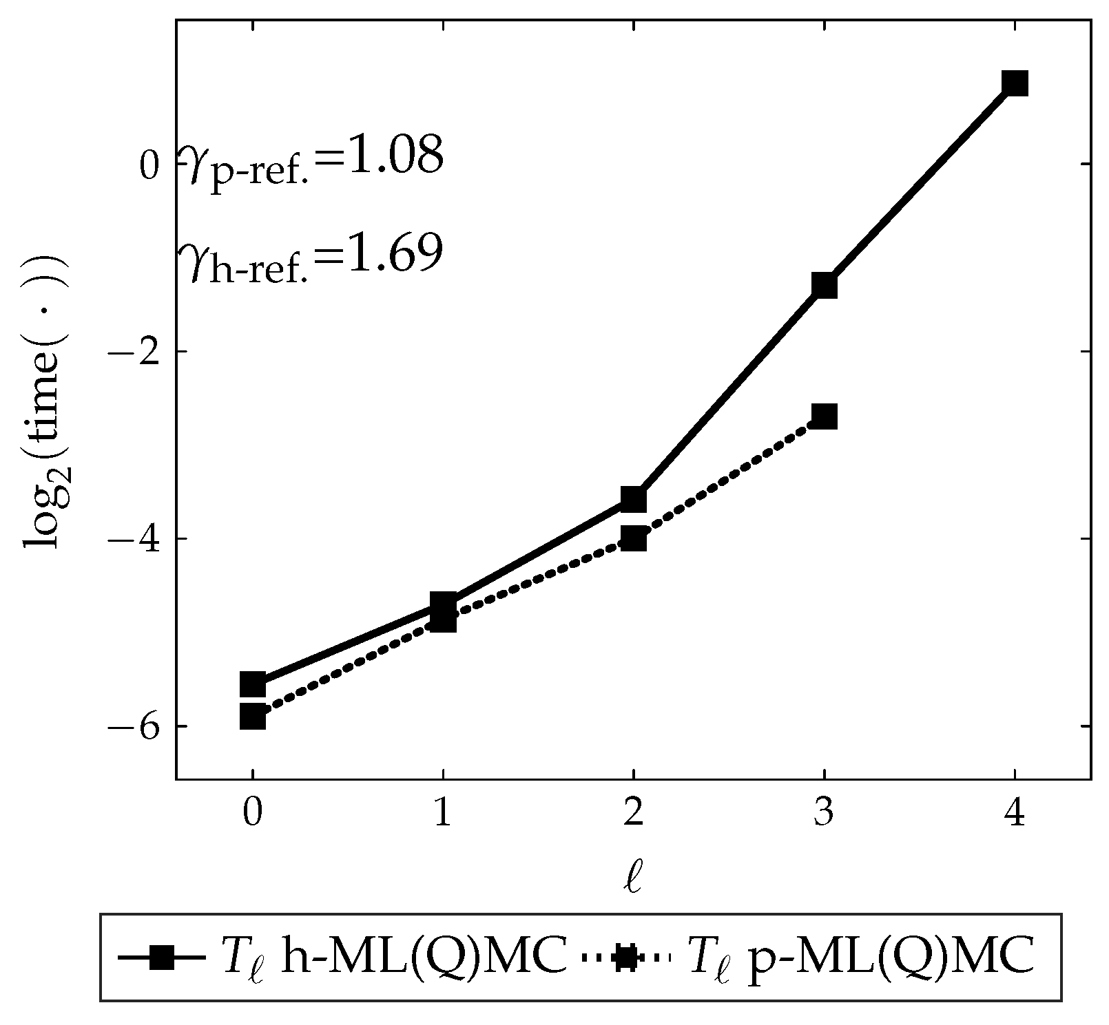
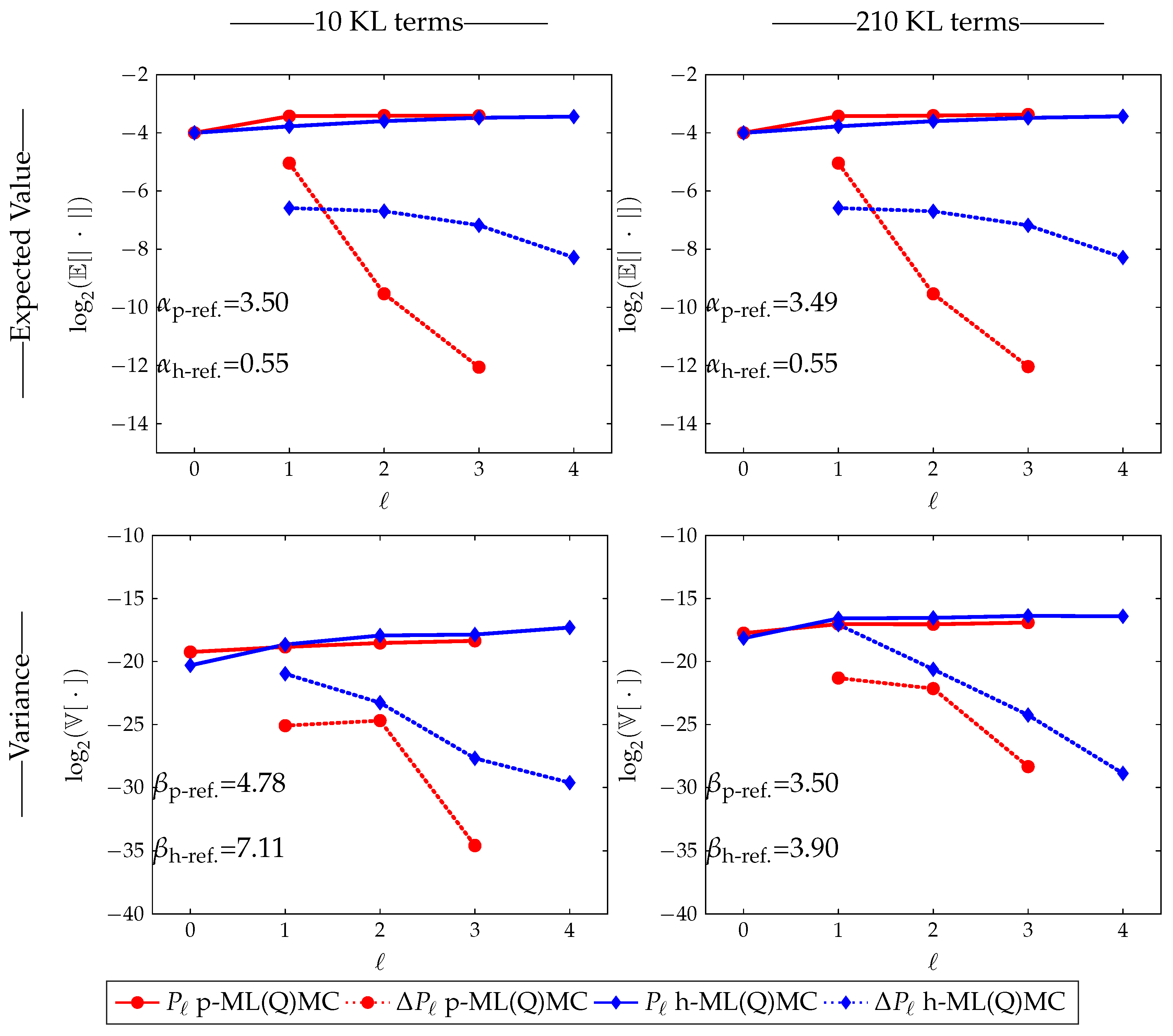
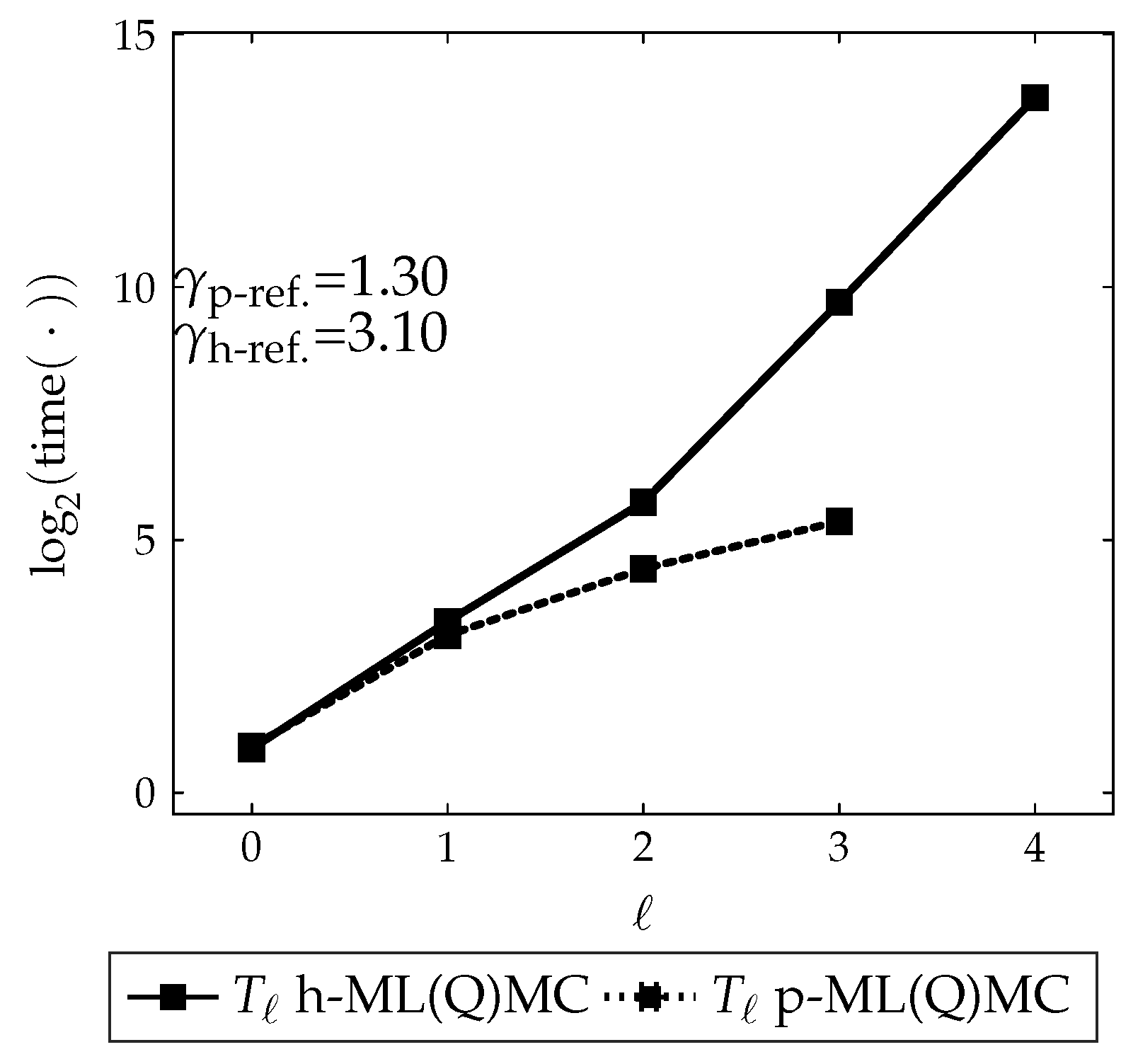
Then, there exists a positive constant $c_4$ such that for any $ϵ<exp(-1)$ there exists an L and a sequence ${\left\{N_{\ell }\right\}}_{\ell =0}^L$ for which the multilevel estimator, $Q_L^{\mathrm{ML}\left(\mathrm{Q}\right)\mathrm{MC}}$ has an $\mathrm{MSE}\le {ϵ}^2$, and

$$\mathrm{cost}(Q^{\mathrm{ML}\left(\mathrm{Q}\right)\mathrm{MC}})\le \left\{\begin{array}{ccc}{c}_4{ϵ}^{-2\delta }\hfill & \hfill & \mathrm{if}\delta \beta >\gamma ,\hfill \\ c_4{ϵ}^{-2\delta }{\left(logϵ\right)}^{1+\delta }\hfill & \hfill & \mathrm{if}\delta \beta =\gamma ,\hfill \\ c_4{ϵ}^{-2\delta -\left(\gamma -\delta \beta \right)/\alpha }\hfill & \hfill & \mathrm{if}\delta \beta <\gamma .\hfill \end{array}\right.$$

(19)

The constant $\alpha$ in Assumption 1 of Theorem 1, represents the rate at which $\mathbb{E}\left[\Delta P_{\ell }\right]$ decreases with increasing level ℓ. The constant $\beta$ in Assumption 2, stands for the decay rate of ${\mathcal{V}}_{\ell }$, i.e., the variance of the estimator of the difference on level ℓ. The constant $\gamma$ in Assumption 3, is determined by the efficiency of the solver. This factor will be different for h-refinement and p-refinement. All three factors will be estimated on the fly in our numerical experiments. The parameter $\delta$ depends on the Quasi-Monte Carlo (QMC) rule used.

The theorem can now be interpreted as follows. When the variance ${\mathcal{V}}_{\ell }$ decreases faster with increasing level ℓ than the cost increases, i.e., $\delta \beta >\gamma$, the dominant computational cost is located on the coarsest level, which is small because $C_0$ is small. Conversely, if the variance decreases slower with increasing level ℓ than the cost increases, i.e., $\delta \beta <\gamma$, the dominant computational cost will be located on the finest level. The cost will be small because ${\mathcal{V}}_L$ is small.

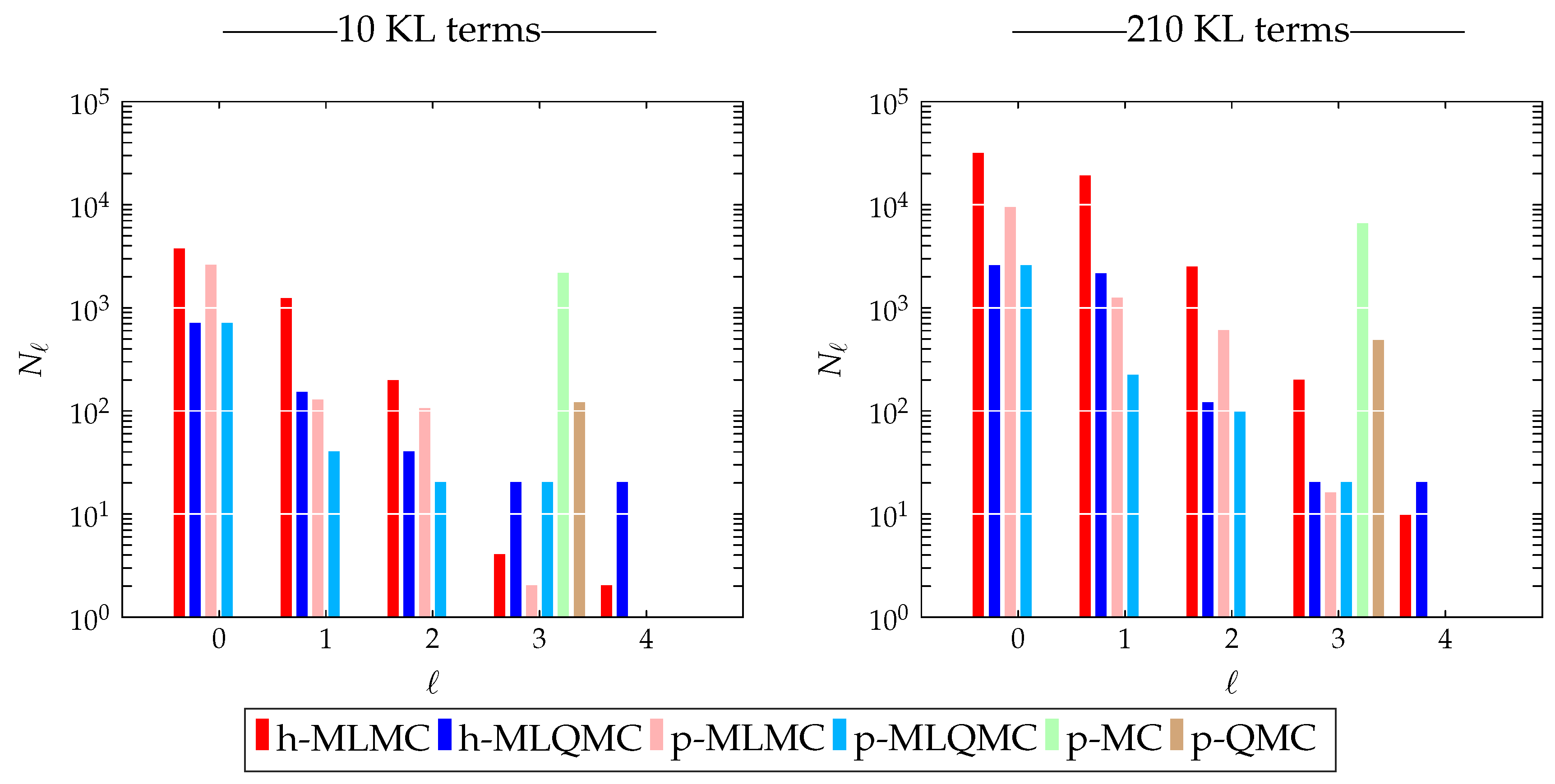
Observe that if $\mathbb{E}\left[P_{\ell }\right]\to \mathbb{E}\left[P\right]$, then $V_{\ell }\to 0$, see Equation (7), as ℓ increases. Hence, the number of samples $N_{\ell }$ will be a decreasing function of ℓ. This means that most samples will be taken on the coarse mesh, where samples are cheap, whereas increasingly fewer samples are required on the finer, but more expensive meshes. In practice, the number of samples must be truncated to $\lceil N_{\ell }\rceil$, the smallest integer larger than or equal to $N_{\ell }$.

Using Equation (10), the total cost of the MLMC estimator, from Equation (8), can be written as

$$\cos \mathrm{t}\left(Q^{\mathrm{MLMC}}\right)=\frac{2}{{ϵ}^2}{\left(\sum _{\ell =0}^L\sqrt{V_{\ell }{C}_{\ell }}\right)}^2.$$

(20)

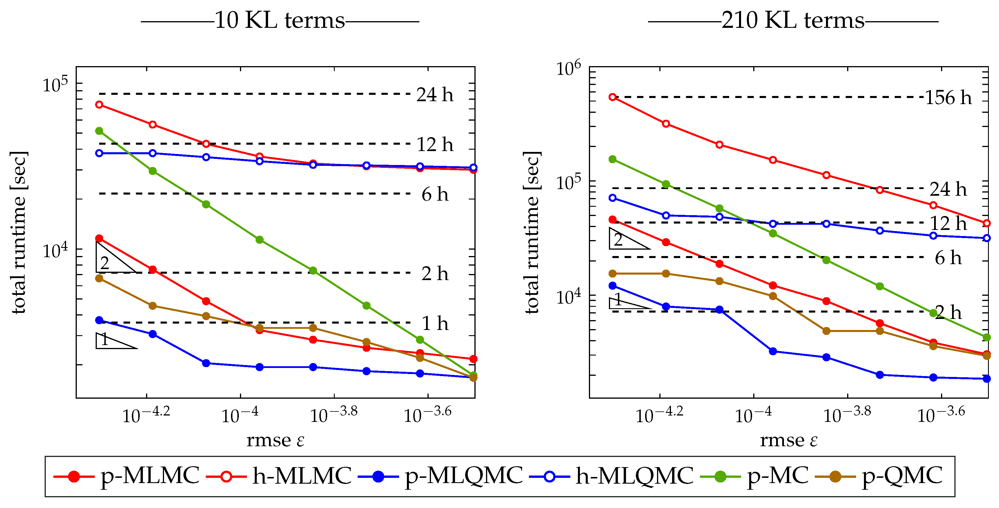
Following this theorem, we note that the optimal cost of the MLMC estimator, which corresponds to $\delta =1$, is proportional to ${ϵ}^{-2}$ when the variance over the levels decreases faster than the cost per level increases, i.e., $\beta >\gamma$. Similarly for the MLQMC estimator, we can hope to achieve an optimal cost proportional to ${ϵ}^{-1}$. Note that this is only true in the limit when $\delta \to 1/2$. We will show in our numerical experiments that the theoretically derived asymptotic cost complexity is close to what we observe. Quasi-Monte Carlo methods work so well because they are based on the concept of weighted function spaces and low effective dimension. Not all higher stochastic dimensions are of equal importance. A series of decreasing weights can be used to quantify this importance. The idea is then to analyze the problem at hand in this weighted function space. The weights can be used to design a good lattice rule that yields a good convergence of the QMC method. A more thorough analysis can be found in [28,30,31].

2.5. Modeling the Spatial Variability

The uncertain spatial variability of the Young’s modulus (model problem 1) and the soil’s cohesion (model problem 2) is represented by means of a random field. The Young’s modulus is represented as a gamma random field, while the soil’s cohesion is represented as a lognormal random field. The starting point for the construction of both fields is the generation of a (truncated) Gaussian random field. This is done by using a Karhunen–Loève (KL) expansion, see [32].

Consider a Gaussian random field $Z(\mathbf{x},\omega )$, where $\omega$ is a random variable with a given covariance kernel. For both cases we choose the Matérn covariance kernel,

$$C(\mathbf{x},\mathbf{y}):={\sigma }^2\frac{1}{2^{\nu -1}\mathsf{\Gamma }\left(\nu \right)}{\left(\sqrt{2\nu }{\displaystyle \frac{{∥\mathbf{x}-\mathbf{y}∥}_2}{\lambda }}\right)}^{\nu }{K}_{\nu }\left(\sqrt{2\nu }{\displaystyle \frac{{∥\mathbf{x}-\mathbf{y}∥}_2}{\lambda }}\right),$$

(21)

with $\nu$ the smoothness parameter, $K_{\nu }$ the modified Bessel function of the second kind, ${\sigma }^2$ the variance and $\lambda$ the correlation length. The parameter values, $\nu$, $\lambda$ and $\sigma$ will be given later on for both cases. The KL expansion can be formulated as:

$$Z(\mathbf{x},\omega )=\overline{Z}\left(\mathbf{x}\right)+\sum _{n=1}^{\infty }\sqrt{{\theta }_n}{\xi }_n\left(\omega \right)b_n\left(\mathbf{x}\right).$$

(22)

Here, $\overline{Z}\left(\mathbf{x}\right)$ denotes the mean of the field, and is set to zero. The ${\xi }_n\left(\omega \right)$ denote i.i.d. standard normal random variables. The symbols ${\theta }_n$ and $b_n\left(\mathbf{x}\right)$ respectively denote the eigenvalues and eigenfunctions of the covariance kernel corresponding to Equation (21). They are the solutions of the eigenvalue problem

$${\int }_{D}C(\mathbf{x},\mathbf{y})b_n\left(\mathbf{y}\right)\mathrm{d}\mathbf{y}={\theta }_n{b}_n\left(\mathbf{x}\right).$$

(23)

These can be approximated by means of a numerical collocation scheme, i.e., by solving

$${\int }_{D}C({\mathbf{x}}_k,\mathbf{y})b_n\left(\mathbf{y}\right)\mathrm{d}\mathbf{y}={\theta }_n{b}_n\left({\mathbf{x}}_k\right),k=1,2,\cdots ,M,$$

(24)

in some well-chosen collocation points ${\mathbf{x}}_k$. Following the Nyström method, see [33], the integral in Equation (24), is approximated by a numerical integration scheme which uses the collocation points as quadrature nodes, i.e.,

$$\sum _{q=1}^M{w}_{q}C({\mathbf{x}}_k,{\mathbf{y}}_q)\widetilde{b_n}\left({\mathbf{y}}_q\right)={\tilde{\theta }}_n\widetilde{b_n}\left({\mathbf{x}}_k\right),k=1,2,\cdots ,M.$$

(25)

In matrix notation, this becomes

$$\Sigma W{\tilde{B}}_n={\tilde{\theta }}_n{\tilde{B}}_n,$$

(26)

where $\Sigma$ is a symmetric positive semi-definite matrix with entries ${\Sigma }_{k,q}=C({\mathbf{x}}_k,{\mathbf{y}}_q)$, W is a diagonal matrix containing the weights $w_q$ on its diagonal and ${\tilde{B}}_n$ is a vector with entries ${\tilde{B}}_{n,q}={\tilde{b}}_n\left({\mathbf{y}}_q\right)$. The matrix eigenvalue problem, Equation (26), can be reformulated as

$$\mathsf{\Psi }{\tilde{B}}_n^{*}={\tilde{\theta }}_n{\tilde{B}}_n^{*},$$

(27)

where ${\tilde{B}}_n^{*}=\sqrt{W}{\tilde{B}}_n$ and $\mathsf{\Psi }=\sqrt{W}\Sigma \sqrt{W}$. Matrix $\mathsf{\Psi }$ is symmetric positive semi-definite. This implies that the eigenvalues ${\tilde{\theta }}_n$ are nonnegative real and the eigenvectors ${\tilde{B}}_n^{*}$ are orthogonal to each other. Using Equation (25), the Nyström eigenfunctions ${\tilde{b}}_n\left(\mathbf{x}\right)$ are obtained:

$${\tilde{b}}_n\left(\mathbf{x}\right)=\frac{1}{{\tilde{\theta }}_n}\sum _{q=1}^M\sqrt{w_q}{\tilde{B}}_{n,q}^{*}C(\mathbf{x},{\mathbf{y}}_q),$$

(28)

where ${\tilde{B}}_{n,q}^{*}$ stands for the q-th element of eigenvector ${\tilde{B}}_n^{*}$. These eigenvalues and eigenfunctions can be used as an approximate eigenpair in the KL expansion after a suitable normalization.

In an actual implementation, the number of KL terms in Equation (22) is truncated to a finite value s, representing the stochastic dimension, i.e.,

$$Z(\mathbf{x},\omega )=\overline{Z}\left(\mathbf{x}\right)+\sum _{n=1}^s\sqrt{{\theta }_n}{\xi }_n\left(\omega \right)b_n\left(\mathbf{x}\right).$$

(29)

The transformation of a Gaussian random field to respectively a gamma and a lognormal random field is detailed in Section 3.1.4 and Section 3.3.4.

2.6. Incorporating the Uncertainty in the Model

By using the Galerkin–Ritz variational formulation of the underlying weak form of the PDE describing the displacement, a system of equations as in Section 3.1.2 or Section 3.3.2 is obtained. This discrete form allows one to incorporate the uncertainty, modeled by means of the random fields, in the finite element model. This is achieved by assigning the discrete values of the random field to each element. For h-ML(Q)MC, this is accomplished by means of the midpoint approach, i.e., the value of the random field is taken constant within each individual element and equal to the value of the realization of the random field at the center point of the element [34]. For p-ML(Q)MC, this is accomplished by means of the integration point method, i.e., the uncertainty is taken into account by its closest quadrature point, see Figure 5 and Figure 6, when numerically integrating the element stiffness matrix by use of Gauss quadrature points [35]. In Figure 9, we show the realization of a gamma random field for three successive levels in case of h-refinement. Figure 10 shows a realization of a lognormal random field for model problem 2 on four successive levels.

It should be stressed that because of the telescoping sum property, i.e., Equation (2), we are free to choose the stochastic model on the different levels, i.e., we do not need to resolve all fine scale features of the random field on the coarse meshes. This is the case, for example, if we vary the number of KL terms, or equivalently, if we use random fields with an artificially enlarged correlation length. The advantage of the latter strategy is that it typically leads to improved convergence rates, $\alpha$, and $\beta$. We refer to [36] Section 4, where this technique was successfully used for highly oscillatory random fields that vary on a fine scale. The artificial smoothing of the random field allows one to choose much coarser meshes than would otherwise be expected from the correlation length of the random field. A complete error analysis can be found in [36,37].

3. Model Problems and Numerical Results

In this section, we describe two model problems, and discuss some numerical results. For both, we benchmark the p-MLQMC algorithm against standard MLMC. First, we introduce the problem. We describe the model, and then expand on the technicalities of the finite element method. Hereafter we introduce the mesh hierarchies. We continue by elaborating on the construction of the model problem specific random fields and conclude by giving the quantity of interest (QoI). Second we present the numerical results. We start by giving estimates for the rates ($\alpha$, $\beta$, $\gamma$) from Theorem 1 in Section 2.4. Next, we present the number of samples for the finest considered tolerance on the MSE. Then, we show how the uncertainty propagates towards the solution, i.e., the uncertainty that is present on the QoI. Lastly, we compare our p-MLQMC algorithm against the different other methods in terms of total simulation time. We first fully discuss the results for model problem 1 before following the same approach for model problem 2.

All the results have been computed on a workstation equipped with 2 physical cores, Intel Xeon E5-2680 v3 CPU’s, each with 12 logical cores, clocked at 2.50 GHz, and a total of 128 GB RAM.

3.1. Model Problem 1

3.1.1. Description

The academic problem we consider consists of the deflection of a cantilever beam clamped at both sides as seen in Figure 11, assuming plane stress, i.e., no stress component in its depth. The beam has a length of $5.0\mathrm{m}$, a height of $1.0\mathrm{m}$, and a width of $0.25\mathrm{m}$. The material is concrete with parameters as follows: a mass density of $2500\mathrm{kg}/{\mathrm{m}}^3$, a Poisson ratio of $0.15$ and a Young’s modulus subject to uncertainty, as specified below. The load of $10.000\mathrm{kN}$ is acting at mid-span. We consider a linear elastic and isotropic material model for this problem.

3.1.2. Finite Element Method

The Finite Element method will be used to compute the displacement of the beam assuming plane stress. An equidistant, regular rectangular mesh consisting of Lagrange quadrilateral elements is employed. The underlying equations and solution methods are reviewed hereunder.

The system equation is of the form

$$\mathbf{K}\underline{\mathbf{u}}=\underline{\mathbf{f}},$$

(30)

with $\mathbf{K}$ the global stiffness matrix, $\underline{\mathbf{f}}$ the global nodal force vector and $\underline{\mathbf{u}}$ the displacement. The global stiffness matrix and nodal force vector are obtained from the element stiffness matrices ${\mathbf{K}}^{\mathbf{e}}$ and the element force vectors ${\underline{\mathbf{f}}}^{\mathbf{e}}$. These are computed numerically by evaluation of the following integrals by means of Gauss quadrature:

$${\mathbf{K}}^{\mathbf{e}}={\int }_{\mathsf{\Omega }}{\mathbf{B}}^T\mathbf{D}\mathbf{B}d\mathsf{\Omega }\mathrm{and}{\underline{\mathbf{f}}}^{\mathbf{e}}={\int }_{{\mathsf{\Gamma }}_t}{\mathbf{N}}^T{\overline{\mathbf{t}}}_{n}d{\mathsf{\Gamma }}_t.$$

(31)

The element nodal force vector ${\underline{\mathbf{f}}}^{\mathbf{e}}$ is modeled as a Neumann boundary condition, where ${\overline{\mathbf{t}}}_n$ stands for the surface traction, specified as a force per unit area, and $\mathbf{N}$ is the element shape function matrix, integrated over the free element boundary ${\mathsf{\Gamma }}_t$. The element stiffness matrix ${\mathbf{K}}^{\mathbf{e}}$ is obtained by integrating the matrix ${\mathbf{B}}^{\mathbf{T}}\mathbf{DB}$ over the element’s surface $\mathsf{\Omega }$. Matrix $\mathbf{B}$ is defined as $\mathbf{LN}$ with $\mathbf{L}$ the derivative matrix specified below. $\mathbf{D}$ is the elastic constitutive matrix for plane stress, containing the element-wise material parameters,

$$\mathbf{L}=\left[\begin{array}{cc}\frac{\partial }{\partial x}& 0\\ 0& \frac{\partial }{\partial y}\\ \frac{\partial }{\partial y}& \frac{\partial }{\partial x}\end{array}\right]\mathrm{and}\mathbf{D}={\displaystyle \frac{E}{1-{\nu }^2}}\left[\begin{array}{ccc}1& \nu & 0\\ \nu & 1& 0\\ 0& 0& {\displaystyle \frac{1-\nu }{2}}\end{array}\right].$$

(32)

3.1.3. Mesh Discretization

The beam model is discretized by a succession of structured nested quadrilateral meshes. We consider two different types of mesh discretization: h-refinement and p-refinement. MLMC and MLQMC will be applied to both refinement schemes. These combinations result in h-ML(Q)MC and p-ML(Q)MC. For h-ML(Q)MC, the coarsest mesh is chosen such that the beam is discretized by at least four elements over the height and twenty elements over the length. Similarly, the discretization for p-ML(Q)MC consists of four elements over the height and twenty elements over the length. This discretization remains the same for all levels. Table 1 lists the number of elements (Nel), degrees of freedom (DOF), the element order per level (Order), and the number of quadrature points per element (Nquad) for h-ML(Q)MC and p-ML(Q)MC. The mesh hierarchies are shown in Figure 1 and Figure 3.

3.1.4. Modeling the Spatial Variability

We select a correlation length $\lambda =0.3$, a standard deviation $\sigma =1.0$ and a smoothness factor $\nu =0.6$ for the covariance kernel in Equation (21) and generation of the Gaussian random field according to Equation (22). We will perform simulations with two different stochastic dimensions. A high stochastic dimension $s=586$ and a moderate stochastic dimension $s=78$. The value $s=586$ accounts for 98% of the variance in the random field, while $s=78$ only accounts for 92%, see Figure 12.

Once the Gaussian field has been generated, a memoryless transformation is applied pointwise, i.e.,

$$g\left(y\right)=F^{-1}\left[\mathsf{\Phi }\left(y\right)\right],$$

(33)

in order to obtain the gamma random field, see [38] for details.

Here, F denotes the marginal cumulative density function (CDF) of the target distribution, $\mathsf{\Phi }$ denotes the marginal CDF of the standard normal distribution, and y is a discrete value of a realization of the random field. The memoryless transformation is depicted in Figure 13, with the solid line representing F, and the dashed line representing $\mathsf{\Phi }$. The characteristics of the Gamma distribution used to represent the uncertainty in concrete are as follows: a mean of $30\mathrm{GPa}$ and a standard deviation of $7.74\mathrm{GPa}$, see [39]. It is known that such a memoryless transformation distorts the underlying covariance function. In the scope of this paper, we will however not address the correction for this distortion. Instead, we will focus on the multilevel methodology. We refer the reader to [40,41,42,43,44] where iterative methods are described which correct this distortion.

3.1.5. Quantity of Interest

The quantity of interest (QoI) we consider for all Monte Carlo simulations is the vertical displacement of the bottom layer of nodes of the beam, as indicated by arrows in Figure 14. The computed solution on each level is interpolated as if it was computed on the finest level. The MLQMC algorithm automatically chooses the node which has the biggest variance as the determining node for the computation of the required number of samples. By doing so, it is assured that the variance constraint is satisfied for all the other nodes.

3.2. Numerical Results for Model Problem 1

3.2.1. Rates

Figure 15 shows the value of $\mathbb{E}\left[P_{\ell }\right]$, $\mathbb{E}\left[\Delta P_{\ell }\right]$, $\mathbb{V}\left[P_{\ell }\right]$ and $\mathbb{V}\left[\Delta P_{\ell }\right]$ as a function of ℓ for a user requested tolerance on the RMSE of 2 × ${10}^{-5}$ for a moderate and a high stochastic dimension. Note that $\mathbb{E}\left[P_{\ell }\right]$ and $\mathbb{V}\left[P_{\ell }\right]$ remain constant across the levels, while $\mathbb{E}\left[\Delta P_{\ell }\right]$ and $\mathbb{V}\left[\Delta P_{\ell }\right]$ decrease for increasing ℓ. However, we observe for P-ML(Q)MC for the moderate stochastic dimension, a slight increase of $\mathbb{E}\left[\Delta P_L\right]$ with respect to $\mathbb{E}\left[\Delta P_{L-1}\right]$. However, this does not impact the results seeing that the overall descend of $\mathbb{E}\left[\Delta P_{\ell }\right]$ is guaranteed, i.e., $\mathbb{E}\left[\Delta P_0\right]>\mathbb{E}\left[\Delta P_L\right]$. The rates $\alpha$ and $\beta$ are included in the figures for h-ML(Q)MC and p-ML(Q)MC. These rates respectively represent the slopes of $\mathbb{E}\left[\Delta P_{\ell }\right]$ and $\mathbb{V}\left[\Delta P_{\ell }\right]$. Figure 16 shows the cost of one solve per level, expressed as the runtime in seconds on a ${\log }_2$ scale. It is logical that per increasing level, the cost increases. This is because the stiffness matrix of the problem becomes larger due to a higher number of finite elements used to discretize the problem for h-ML(Q)MC. For p-ML(Q)MC this is due to a higher number of nodes. We observe that the cost per increasing level for p-ML(Q)MC grows slower than for h-ML(Q)MC. Combining this with the fact that the values of $\mathbb{V}\left[\Delta P_{\ell }\right]$ for p-ML(Q)MC are smaller than for h-ML(Q)MC, i.e., less samples are to be taken, we can expect that p-ML(Q)MC will outperform h-ML(Q)MC.

We can now evaluate in which regime, according to Theorem 1, h-ML(Q)MC and p-ML(Q)MC operate. We find for the moderate stochastic dimension that $\beta >\gamma$ for both h- and p-ML(Q)MC. We thus expect the h-MLMC and p-MLMC cost to be proportional to ${ϵ}^{-2}$. For the high stochastic dimension, we find that $\beta >\gamma$ for p-MLMC and $\beta <\gamma$ for h-MLMC. We respectively expect a cost proportional to ${ϵ}^{-2}$ and ${ϵ}^{-2.05}$. The cost for p-MLQMC and h-MLQMC cannot be evaluated from this figure, because no rate $\delta$ is available. The rate $\delta$ appears as an exponent in the integration error bound for QMC, see [28], and is not shown here.

3.2.2. Number of Samples

Figure 17 shows the total number of samples over the different levels for a user requested tolerance on the RMSE of 2 × ${10}^{-5}$ for a moderate and a high stochastic dimension, for the different methods. The number of samples is decreasing as the level ℓ increases. Samples on lower levels are computationally less expensive. It is therefore advantageous to have a high number of samples on lower levels. Also, it can be seen that the sample sizes for MLQMC are lower than for MLMC. This is because the MLQMC sample points are chosen deterministically in an optimal way. This will result in a lower total computation time for MLQMC. The number of samples for p-ML(Q)MC is lower than for its respective h-ML(Q)MC counterpart. The origin of this effect is to be found in a lower value of $\mathbb{V}\left[\Delta P_{\ell }\right]$. We also see that for the high stochastic dimension, h-ML(Q)MC needs a total of 5 levels to satisfy its bias condition. This is to be compared with p-ML(Q)MC, which only needs a total of 4 levels, regardless of the considered stochastic dimension. Also observe that the samples for h-MC, p-MC, h-QMC and p-QMC are located on the finest level.

3.2.3. Uncertainty Propagation in the Solution

Figure 18 shows the uncertainty propagation towards the solution, i.e., the uncertainty on the QoI for the moderate and high stochastic dimension. Darker shades of blue indicate a higher probability for the displacement. The orange full line represents the mean, together with the 1-$\sigma$ bounds in dashed orange.

3.2.4. Runtime

We plot the runtimes of the different methods in Figure 19. We compare the p-MLQMC method against p-MLMC and h-ML(Q)MC. As a reference we also plot the times for h-MC, p-MC, h-QMC and p-QMC. The p-MLQMC method consistently outperforms all the other methods. In case of a moderate stochastic dimension we observe a gain of a factor 20 with respect to h-MLMC. For a high stochastic dimension, we observe a gain of a factor 100 with respect to h-MLMC. We also observe that all MLMC simulations exhibit a cost proportional to ${ϵ}^{-2}$, as expected. The MLQMC simulations on the other hand, exhibit a cost in the range of ${ϵ}^{-1}$ to ${ϵ}^{-2}$, depending on the stochastic dimension. Interestingly, we note that for a moderate stochastic dimension, it remains advantageous to use h-MLQMC. The total runtime for h-MLQMC is indeed lower than for p-MLMC. This advantage, however, disappears for the high stochastic dimension. Here, all p-ML(Q)MC and p-MC simulations outperform the h-ML(Q)MC and h-MC simulations. p-MC even outperforms all h-ML(Q)MC simulations. This is due to the extra levels for the h-ML(Q)MC and h-MC simulations which are needed in order to satisfy their bias constraint.

3.2.5. Level Adaptivity

In order to better illustrate the level adaptivity of Algorithm 1, we have rerun Algorithm 2 to generate more meshes that can be used in our p-MLQMC method. The details of the hierarchy can be found in

Table 3. Number of elements, degrees of freedom, element order and number of quadrature points for model problem 1 for additional tolerances.

	p-ML(Q)MC
Level	Nel	DOF	Order	Nquad
0	80	210	1	25
1	80	738	2	81
2	80	1586	3	121
3	80	2754	4	225
4	80	4242	5	289
5	80	6050	6	441
6	80	8178	7	625
7	80	10,626	8	729

. We will simulate model problem 1 for finer tolerances. In order to more easily show that an extra level is added, we have set $\sigma =1.5$ in Equation (21). This has an impact on the bias.

In Figure 20, we show the runtime and the sample sizes for finer considered tolerances than in Figure 19, for a moderate stochastic dimension. We observe a cost in the range of ${ϵ}^{-1}$ to ${ϵ}^{-2}$.

In Figure 21, we show the runtime and the sample sizes for finer considered tolerances than in Figure 19, for a high stochastic dimension. Here, we observe a cost that is closer to ${ϵ}^{-2}$ than to ${ϵ}^{-1}$. Two extra levels are adaptively added in order to satisfy the bias constraint.

3.3. Model Problem 2

3.3.1. Description

Model problem 2 is a slope stability problem where the soil’s cohesion has a spatially varying uncertainty [45]. In a slope stability problem, a sufficient factor of safety is required against sliding failure of the soil. However, this is complicated by a high level of heterogeneity and corresponding uncertainty of the soil’s strength parameters [45]. The spatial dimensions of the slope are: a length of $20\mathrm{m}$, a height of $14\mathrm{m}$ and a slope angle of 30°. The material characteristics are: a Young’s modulus of $30\mathrm{MPa}$, a Poisson ratio of $0.25$, a density of $1330\mathrm{kg}/{\mathrm{m}}^3$ and a friction angle of 20°. Plane strain is considered for this problem, i.e., no strain component in its depth.

3.3.2. Finite Element Method

Because of the nonlinear stress-strain relation in the plastic domain, a Newton–Raphson iterative solver is used. The plastic region is governed by the Drucker–Prager yield criterion with a small amount of isotropic linear hardening for numerical stability reasons. An incremental load approach is used starting with a force of $0\mathrm{N}$ until the downward force resulting from the slope’s weight is reached. The methods used to solve the slope stability problem are based on ([46], Chapter 2 Section 4, and Chapter 7 Sections 3 and 4). For this case, the system equation takes the following form:

$$\mathbf{K}\Delta \underline{\mathbf{u}}=\underline{\mathbf{r}},$$

(34)

where $\Delta \underline{\mathbf{u}}$ stands for the displacement increment. The vector $\underline{\mathbf{r}}$ is the residual,

$$\underline{\mathbf{r}}=\underline{\mathbf{f}}+\Delta \underline{\mathbf{f}}-\underline{\mathbf{q}},$$

(35)

where $\underline{\mathbf{f}}$ stands for the sum of the external force increments applied in the previous steps, $\Delta \underline{\mathbf{f}}$ for the applied load increment of the current step and $\underline{\mathbf{q}}$ for the internal force resulting from the stresses

$$\underline{\mathbf{q}}={\int }_{\mathsf{\Omega }}{\mathbf{B}}^T\mathbf{\sigma }d\mathsf{\Omega }.$$

(36)

First, the displacement increment of all the nodes is computed according to Equation (34), with an initial system stiffness matrix $\mathbf{K}$ resulting from the assembly of the element stiffness matrix ${\mathbf{K}}^{\mathbf{e}}$, computed by means of a Gauss quadrature, i.e.,

$${\mathbf{K}}^{\mathbf{e}}={\int }_{\mathsf{\Omega }}{\mathbf{B}}^T{\mathbf{D}}^{\mathrm{ep}}\mathbf{B}d\mathsf{\Omega }.$$

(37)

Here ${\mathbf{D}}^{\mathrm{ep}}$ denotes the elastoplastic constitutive matrix. The initial state of ${\mathbf{D}}^{\mathrm{ep}}$ is defined as

$${\mathbf{D}}^{\mathrm{ep}}={\displaystyle \frac{E(1-\nu )}{(1+\nu )(1-2\nu )}}\left[\begin{array}{ccc}1& {\displaystyle \frac{\nu }{(1-\nu )}}& 0\\ {\displaystyle \frac{\nu }{(1-\nu )}}& 1& 0\\ 0& 0& {\displaystyle \frac{(1-2\nu )}{2(1-\nu )}}\end{array}\right].$$

(38)

Secondly, the strain increment $\Delta \epsilon$ is computed as

$$\Delta \epsilon =\mathbf{B}\Delta \underline{\mathbf{u}}.$$

(39)

Finally, the nonlinear stress–strain relationship,

$$d\mathbf{\sigma }={\mathbf{D}}^{\mathrm{ep}}d\epsilon ,$$

(40)

is integrated by means of a backward Euler method. The backward Euler method essentially acts as an elastic predictor-plastic corrector; an initial stress state that is purely elastic is computed and then projected in the direction of the yield surface to obtain the plastic stress state. Due to the implicit nature of the integrated stress-strain relation, this equation must be supplemented with the integrated form of the hardening rule and the yield condition. This system of nonlinear equations is then solved with an iterative Newton–Raphson method. Afterwards, the consistent tangent stiffness matrix is computed, see [47]. This matrix is then used to compute the updated element stiffness matrix, Equation (37), resulting in an updated system stiffness matrix $\mathbf{K}$. The inner iteration step of solving the stress-strain relation and the updated system stiffness matrix is repeated for each outer iteration step which solves Equation (34). The outer step consists in balancing the internal forces with the external ones as to satisfy the residual, which in our case equals ${10}^{-4}$ multiplied with the load increment. The procedure used is incremental–iterative, relying on the iterative Newton–Raphson method. This process is repeated for each load increment.

3.3.3. Mesh Discretization

The problem is discretized by means of a hierarchy of unstructured triangular nested meshes. Both h-ML(Q)MC and p-ML(Q)MC will be applied. Table 2 lists the number of elements (Nel), degrees of freedom (DOF), element order per level (Order), and the number of quadrature points per element (Nquad) for h-ML(Q)MC and p-ML(Q)MC. The mesh hierarchies are shown in Figure 2 and Figure 4.

3.3.4. Modeling the Spatial Variability

For model problem 2, we select a correlation length $\lambda =1.0$, a standard deviation $\sigma =1.0$ and a smoothness factor $\nu =0.6$ in Equation (21). Here, we also consider two different stochastic dimensions for the Gaussian random field: a value $s=10$, accounting for 92% of the variance, and a value $s=210$, accounting for 99% of the variance, Figure 22.

The obtained Gaussian field is transformed into a lognormal random field by applying the exponential operator,

$$Z_{\mathrm{lognormal}}(\mathbf{x},\omega )=exp\left(Z(\mathbf{x},\omega )\right).$$

(41)

By using this operation, the underlying covariance is not distorted. The characteristics of the lognormal distribution used to represent the uncertainty of the soil’s cohesion are as follows: a mean of $6\mathrm{kPa}$ and a standard deviation of $300\mathrm{Pa}$.

3.3.5. Quantity of Interest

We consider the vertical displacement of the upper left node of the model, see Figure 23, as a quantity of interest.

3.4. Numerical Results for Model Problem 2

3.4.1. Rates

As for model problem 1, we first present the different rates for model problem 2 for a user requested tolerance on the RMSE of 5 × ${10}^{-5}$. These are shown in Figure 24. Here, we observe that the $\alpha$ rates for p-ML(Q)MC exhibit much larger values. The bias constraint will be fulfilled with less levels for p-ML(Q)MC than for h-ML(Q)MC. On the other hand, the $\beta$ rates for p-ML(Q)MC exhibit a smaller value than for h-ML(Q)MC. These results suggest that an approach where both p-refinement and h-refinement are combined would yield a good decrease of $\mathbb{E}\left[\Delta P_{\ell }\right]$ and $\mathbb{V}\left[\Delta P_{\ell }\right]$. Following this figure, we expect that all h-ML(Q)MC simulations will require more levels than their p-ML(Q)MC counterparts to satisfy the bias constraint. We have chosen to limit the amount of levels for the h-ML(Q)MC simulations to a total of five. This is done because of the considerable cost to compute solutions on finer meshes. This inadvertently means that a bias is still present on our h-ML(Q)MC results. Our p-ML(Q)MC solutions do not exhibit such a bias, i.e., the bias constraint is satisfied with a total of four levels. In Figure 25, we again observe that the cost increase, $\gamma$, per increasing level is smaller for p-ML(Q)MC than for h-ML(Q)MC.

3.4.2. Number of Samples

Figure 26 shows the number of samples for a high and a moderate stochastic dimension for model problem 2 for a user requested tolerance on the RMSE of 5 × ${10}^{-5}$. Similar conclusion can be drawn as for model problem 1. Here, our p-ML(Q)MC simulations only need four levels while h-ML(Q)MC requires at least five.

3.4.3. Uncertainty Propagation in the Solution

Figure 27 shows the uncertainty on the QoI. Here the vertical displacement of the QoI is shown in function of the applied force. The line style convention is the same as for model problem 1.

3.4.4. Runtime

We plot the runtimes for the different methods in Figure 28. We show the total runtime in seconds in function of the user requested tolerance. As already observed for model problem 1, p-MLQMC outperforms h-MLMC. For a moderate stochastic dimension we observe a speedup up to a factor 20. For the high stochastic dimension we observe a speedup up to a factor 40. Note however that for the h-ML(Q)MC simulations we have fixed the maximum level because of the prohibitively large computational cost. Because of this, we have chosen not to simulate this case with h-MC or h-QMC. Here, we clearly observe a cost proportional to ${ϵ}^{-1}$ for p-MLQMC.

3.4.5. Level Adaptivity

In order to better illustrate the level adaptivity of Algorithm 1, we have rerun Algorithm 2 to generate more meshes that can be used in our p-MLQMC method. The details of the hierarchy can be found in

Table 4. Number of elements, degrees of freedom, element order and number of quadrature points for model problem 2 for additional tolerances.

	p-ML(Q)MC
Level	Nel	DOF	Order	Nquad
0	33	48	1	7
1	33	160	2	13
2	33	338	3	19
3	33	582	4	25
4	33	892	5	28
5	33	1268	6	33
6	33	1720	7	37
7	33	2218	8	61
8	33	2792	9	73

.

In Figure 29, we show the runtime and the sample sizes for finer considered tolerances than in Figure 28, for a moderate stochastic dimension. We clearly observe a cost proportional to ${ϵ}^{-1}$.

In Figure 30, we show the runtime and the sample sizes for finer considered tolerances than in Figure 28, for a high stochastic dimension. Again, we observe a cost proportional to ${ϵ}^{-1}$. We also observe that additional levels are added adaptively in order to satisfy the bias constraint.

4. Conclusions

In this work we presented a novel multilevel algorithm, p-refined Multilevel Quasi-Monte Carlo. We benchmarked this method against existing multilevel algorithms for two engineering cases: an academic clamped beam bending problem, from the civil/mechanical engineering domain, and the slope stability problem, from the geotechnical engineering domain. We detailed how the random fields are generated for these two cases and how they were taken into account in the model. We also described two algorithms necessary for p-MLQMC, the sample algorithm itself and an algorithm which returns the location of the points where the discrete values of the random field are to be computed. The second algorithm was developed for two dimensional problems but is extensible to three dimensional problems. We observed that the p-MLQMC method drastically reduces the computational cost with respect to a classical Multilevel Monte Carlo approach. We observed computational gains ranging from a factor 20 to 100. In turn, h-MLMC is 4 to 6 times faster than standard MC. In addition to this cost reduction, we also showed that the computational cost increase in function of a user requested tolerance $ϵ$, is proportional to ${ϵ}^{-1}$. For model problem 2, we have shown that the decay of $\mathbb{E}\left[\Delta P_{\ell }\right]$ for h-ML(Q)MC is much slower than for p-ML(Q)MC. The opposite holds for the decay of $\mathbb{V}\left[\Delta P_{\ell }\right]$. This behavior could be exploited in a Multi-Index (Quasi)-Monte Carlo setting in order to further reduce the total computational cost, see [11]. Higher order Quasi-Monte Carlo methods, which use higher order digital nets instead of lattice rules, could be used in order to further decrease the error on the root mean square, and so decrease the computational cost.