Automobile Fine-Grained Detection Algorithm Based on Multi-Improved YOLOv3 in Smart Streetlights


1
School of Information and Communication Engineering, University of Electronic Science and Technology of China, Chengdu 611731, China
2
College of Physics and Electronic Information, Inner Mongolia Normal University, Hohhot 010022, China
*
Authors to whom correspondence should be addressed.
Algorithms 2020, 13(5), 114; https://0-doi-org.brum.beds.ac.uk/10.3390/a13050114
Submission received: 17 March 2020
/
Revised: 28 April 2020
/
Accepted: 29 April 2020
/
Published: 2 May 2020
(This article belongs to the Special Issue Algorithms for Smart Cities)
Abstract
:Upgrading ordinary streetlights to smart streetlights to help monitor traffic flow is a low-cost and pragmatic option for cities. Fine-grained classification of vehicles in the sight of smart streetlights is essential for intelligent transportation and smart cities. In order to improve the classification accuracy of distant cars, we propose a reformed YOLOv3 (You Only Look Once, version 3) algorithm to realize the detection of various types of automobiles, such as SUVs, sedans, taxis, commercial vehicles, small commercial vehicles, vans, buses, trucks and pickup trucks. Based on the dataset UA-DETRAC-LITE, manually labeled data is added to improve the data balance. First, data optimization for the vehicle target is performed to improve the generalization ability and position regression loss function of the model. The experimental results show that, within the range of 67 m, and through scale optimization (i.e., by introducing multi-scale training and anchor clustering), the classification accuracies of trucks and pickup trucks are raised by 26.98% and 16.54%, respectively, and the overall accuracy is increased by 8%. Secondly, label smoothing and mixup optimization is also performed to improve the generalization ability of the model. Compared with the original YOLO algorithm, the accuracy of the proposed algorithm is improved by 16.01%. By combining the optimization of the position regression loss function of GIOU (Generalized Intersection Over Union), the overall system accuracy can reach 92.7%, which improves the performance by 21.28% compared with the original YOLOv3 algorithm.
1. Introduction
With the rapid development of the modern transportation industry, a common scenario in an urban transportation network is that certain sections of the road may experience severe traffic congestion, whereas the traffic flow on nearby sections is relatively smooth. Therefore, by knowing the traffic conditions of each road in real time, the intelligent transportation system can help drivers choose a reasonable driving route, which is also an effective approach to solve urban traffic congestion [1,2,3,4]. The image-processing-based traffic length detection system combines image processing with various traffic information technologies and has the advantages of wide application range, high measurement precision, excellent real-time performance and direct upgrade based on the existing monitoring system. Therefore, it is an important technical component for obtaining modern intelligent traffic information.
During the last decade, researchers have conducted extensive studies. In 2014, Ross Girshick et al. [5] proposed a visual inspection method named R-CNN (Regions with Convolutional Neural Networks features). This method first divides the inspected image into thousands of different regions, then extracts deep features of these regions, and finally adopts Softmax for classification. On dataset VOC2012, the mean average precision (mAP) detected by R-CNN could reach 53.3%, which is higher than the precision of previous methods. However, it has the disadvantages of long detection time and difficult engineering application. In 2016, Liu et al. [6] proposed the SSD (Single-Shot Multi-Box Detector) method, which improves the deep convolutional neural network of VGG-16 (Visual Geometry Group Network) [7] and the target detection method of YOLO (You Only Look Once) [8], extracts multi-scale feature maps, and directly outputs the location and class of the detected target. On dataset VOC2007, this method could achieve a mAP of 74.3% and a speed of 59 FPS. In 2018, Chu et al. [9] reported a deep convolutional neural network (CNN) based on multiple tasks and the vehicle detection method for an automatic pilot based on region-of-interest voting. In this method, the multi-task targets of CNN include area overlapping, subclass, regression of detection frame and region of proposals (ROI) regional training, and the vehicle is detected by fully considering the influence of the neighborhood ROI. According to the validation of vehicle datasets KITTI [10] and VOC [11], it presents a much better performance than most similar algorithms. In 2019, Chang-Yu Cao et al. used the YOLO-UA model to improve the detection precision of vehicles under complicated weather conditions [12].
In the various studies above, all researchers have ignored a problem, which is that, in actual street lighting, we need to extend the effective detection distance of the video as much as possible to reduce the number of intelligent streetlights, and thus reduce the cost of the entire system. However, in the case of long-distance vision, the accuracy of the current algorithm to achieve fine-grained car classification is not ideal. In order to address this issue, in this article, we primarily make the following three contributions:
- In order to realize high-precision and large-scale traffic situation detection, we propose a distributed system based on smart streetlights.
- Based on the dataset UA-DETRAC, we add the local manually labeled data images in the sight of smart streetlights, establish the classification dataset for SUVs, sedans, taxis, commercial vehicles, small commercial vehicles, vans, buses, trucks, and pickup trucks, and build the dataset UA-DETRAC-LITE-NEW.
- We optimize the YOLOv3 algorithm in various respects to improve the detection accuracy for distant cars in the sight of smart lights and then combine it with multi-scale training and anchor clustering methods to improve the accuracy of automobile target detection. In addition, we apply label smoothing and mixup approaches to increase the generalization ability of the model and adopt optimized position regression loss functions of IOU (Intersection Over Union) and GIOU to increase the system accuracy. Each step of the improvement is experimentally verified.
2. Smart Streetlights and Experimental Datasets
2.1. Smart Streetlights
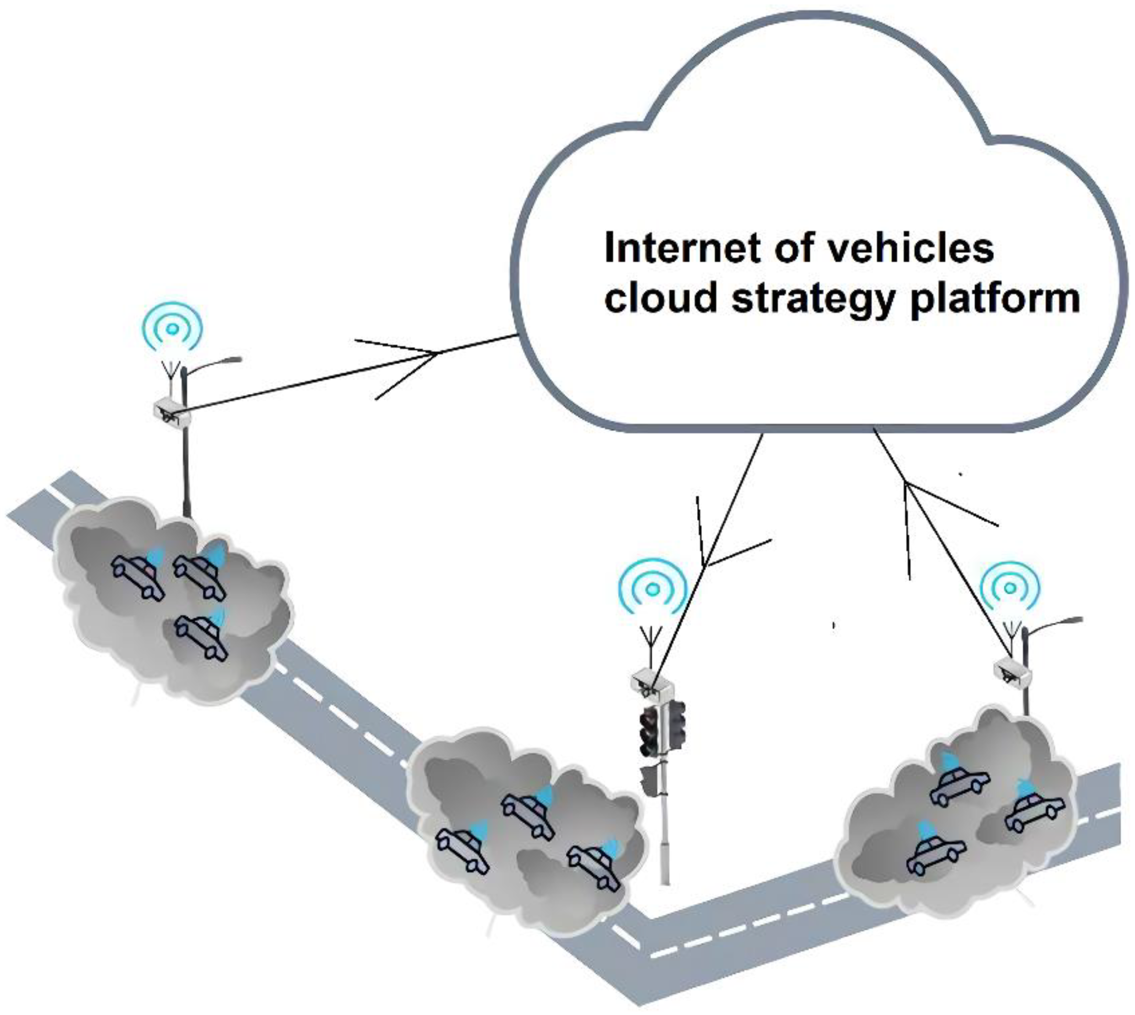
As shown in Figure 1, the camera and computing unit are integrated into the ready-made streetlight to form an intelligent streetlight. After the camera in the intelligent streetlight identifies the type and number of vehicles, the traffic data collected by the computing unit is transmitted to the cloud strategy platform through the wireless communication, power line carrier communication or visible light communication system. According to the information from smart streetlights, the cloud strategy platform could provide a variety of application services, such as traffic guidance and emergency rescue. Because the streetlight system is a complete infrastructure, cable layout and routing have cost advantages. In addition, streetlights can provide sufficient brightness for video and image detection to ensure the accuracy of detection.
Furthermore, the number of nine kinds of vehicles in the field of vision of each streetlight can be summed up, and the ratio of the road area occupied can be accurately calculated according to the area of the road projected by each type of vehicle. This index is very important for illegal parking assessment, traffic diversion and traffic light strategy formulation, which is also difficult to achieve by other technologies (satellite remote sensing, microwave radar).
2.2. Experimental Dataset
The target detection in this research focuses on the fine-grained detection of vehicles, but there is no public fine-grained vehicle detection dataset at present. Therefore, in this paper, the dataset used in the experiment is obtained by mixing the manually labeled dataset with the public dataset.
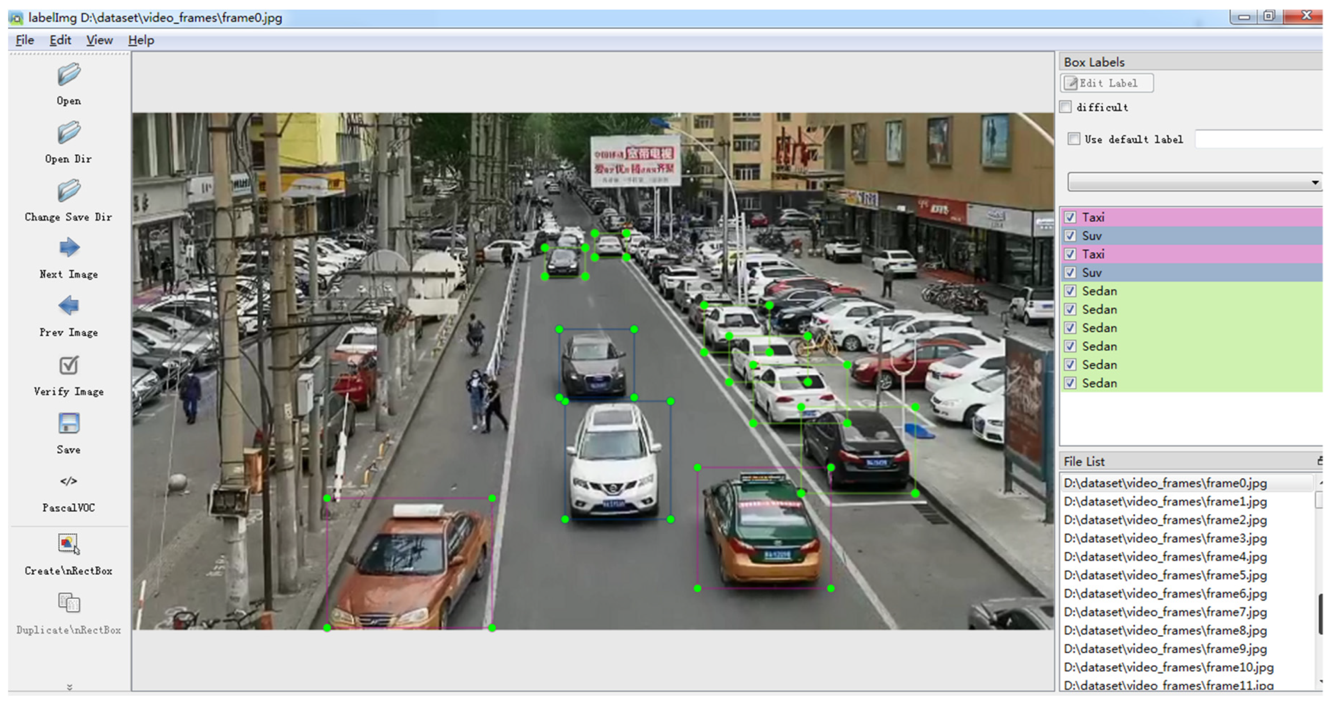
Part of the manually labeled dataset was obtained by the camera installed in a pedestrian bridge in Chengdu. This dataset includes the front and back images of vehicles. The vehicle models include sedans, buses, taxis, trucks, SUVs and pick-ups; the involved scenarios include: daytime, night, fine day and cloudy day. In total, 1231 images were obtained, and the resolution was adjusted to 540 × 960. The other part was obtained through network crawling: 387 images were obtained in total, and the resolution was adjusted to 540 × 960. Finally, the vehicle location was labeled using LabelImage, and the labeled data were given in the format of VOC2007. Figure 2 presents the frame image decomposed from the vehicle video collected from a smart streetlight in Chengdu. The detection range is 67 m.
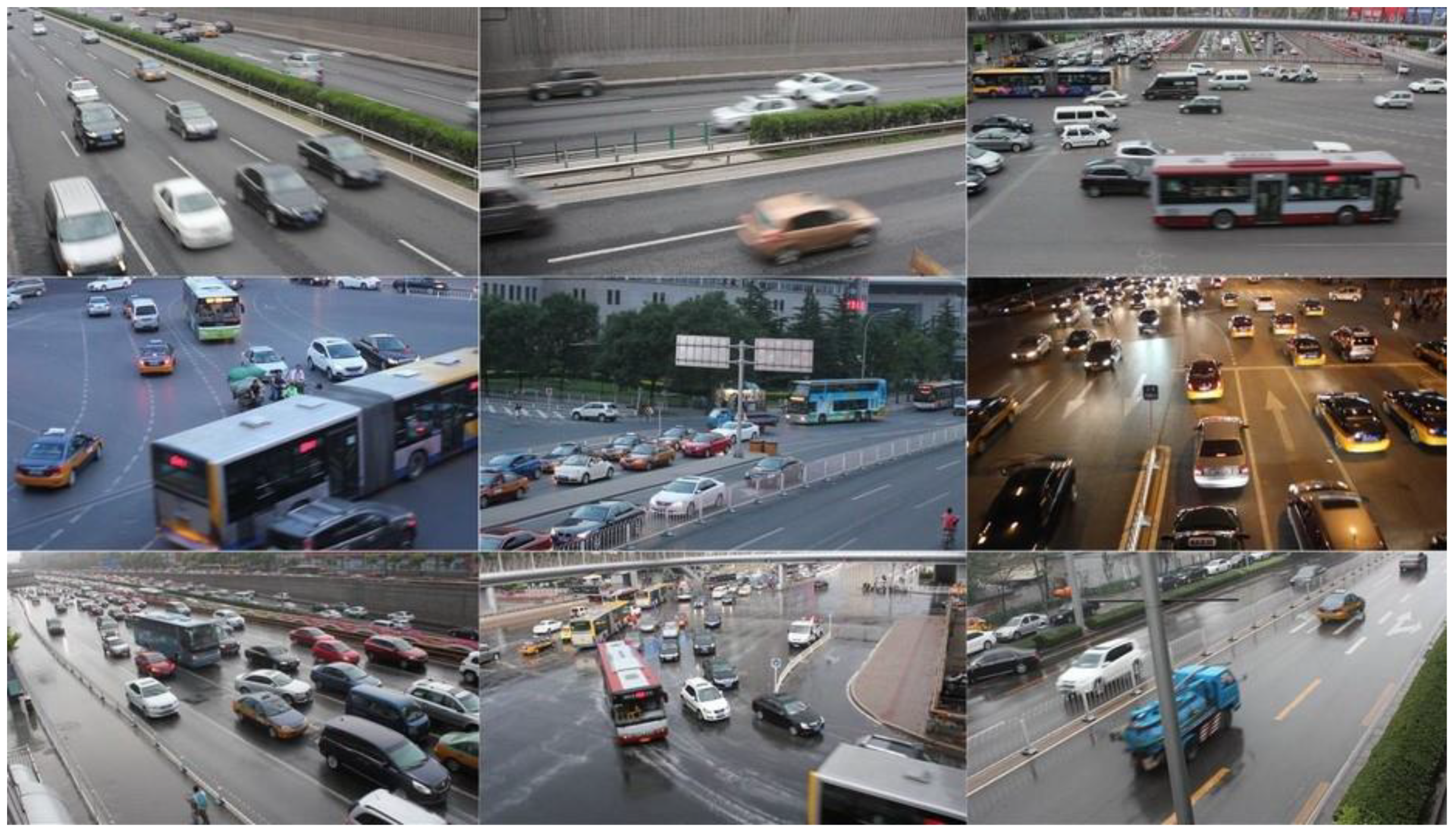
The common public vehicle detection datasets include UA-DETRAC [13,14,15], KITTI [16], etc. Because the images in the dataset UA-DETRAC were all collected from a pedestrian bridge, the image collection angle is closest to the angle of the image collected by intelligent streetlights in the IoV (Internet of Vehicles), so the dataset UA-DETRAC is used in this paper. This dataset consists of ten-hour video continuously collected by a Cannon EOS 550 camera at 24 different locations in Beijing and Tianjin, China. The video was collected at the speed of 25 frames per second (fps); then, each frame of video was decomposed to images using software, and each image had a resolution of 960 × 540 pixels. In this dataset, 8250 vehicles were manually labeled, and there were 1.21 million label boxes in total. The dataset includes the labels of four major classes and thirteen subclasses, such as SUV, sedan, taxi, commercial vehicle, small commercial vehicle, large van, hatchback, bus, police car, medium van, truck, pick-up and platform truck. The shooting scenarios include cloudy weather, night, sunny days and rainy days, as shown in Figure 3.
Because, among the subclasses of vehicles in the dataset UA-DETRAC, the distribution of various types of vehicles is not even in number, the numbers of police cars and platform trucks are particularly low, and there are only 300 labeled police cars in the entire dataset. Furthermore, there are not many police cars on real roads, and manual shooting is inconvenient. Considering the above factors, in this paper, dataset UA-DETRAC only consists of the following nine subclasses of vehicles: SUVs, sedans, taxis, commercial vehicles, small commercial vehicles, vans, buses, trucks and pick-ups, in which the class of vans combines the two subclasses of large vans and medium vans, and trucks combine platform trucks and original trucks. Because the computing resources are not particularly sufficient, in this paper, we select 13,516 images from the 82,118 images in dataset UA-DETRAC, and mix them with 1618 manually labeled images to form the dataset used in this paper: UA-DETRAC-LITE-NEW. Among these, the 2053 manually labeled images are mainly used to supplement the insufficient number of pick-ups and trucks in the original dataset UA-DETRAC. In this paper, we select 12,455 images from the 15,569 in the dataset UA-DETRAC-LITE-NEW as the training dataset, and we select 3114 images captured in the sight of streetlights as the test dataset.
3. Methodology
3.1. Introduction of YOLOv3
In 2018, Joseph Redmon et al. [17] proposed YOLOv3, and, compared with the last generation of the YOLO algorithm, this method has increased detection prevision and strengthened identification ability for small objects. In YOLOv3, a new backbone network called Darknet-53 is used. By referring to the residual network (ResNet [18]), this network has set shortcut connections between some layers, so that information can be directly transmitted from shallow layers to deep layers, so as to maintain the integrity of information. In addition, the idea, similar to FPN [19], is to conduct multi-scale prediction of bounding boxes, which can prevent missing of small objects.
In YOLOv3, the L2 distance is used to calculate the loss by default. Loss consists of three parts: position loss, confidence loss and class loss. The loss computation is as shown in Formula (1):
where YOLOv3 is used to calculate loss. Pay attention to the following details:
- (1)
- During calculation of position loss, the L2 distance does not have scale invariability relative to the bounding box, so the loss of a small bounding box should be distinguished from that of a big bounding box, which is more reasonable. The author multiplies factor α () with the L2 distance loss of position to weaken the negative influence of scale on position loss. and are the width and height of normalized true-value bounding boxes. Factor α is smaller when encountering large-scale targets and bigger when encountering small-scale targets, and in this way, the loss of small bounding boxes can be improved.
- (2)
- During calculation of loss, no matter whether it is position loss or other loss, the true value should correspond to the predicted values one by one to realize calculation. However, in reality, the number of targets in each image is not fixed. When the output image has a scale of 416, assuming m image targets participate in the training, while the YOLOv3 model will predict 10,647 targets, they cannot correspond to each other one by one in this case. Therefore, YOLOv3 employs a matching mechanism to reconstruct m targets in true-value tag into the data in the format of 10,647 targets. m targets are placed in their proper positions in the 10,647 constructed data, and, at this moment, the calculation and training process is completed.
- (3)
- In the YOLOv3 algorithm, only the lattice with the scale which best matches the anchor is used to predict the target. However, under normal circumstances, it is also highly possible to use the lattices near this lattice to predict this target. This situation is normal, which does not require punishing this lattice. However, when the lattice far away from this lattice is also used to predict this target, this situation is abnormal, which requires punishment. Therefore, in YOLOv3, the predicted value and corresponding position of constructed real-value tag are used to calculate IoU, then the IoU is used to decide when punishment is required and when it is not. In general, a hyper-parameter will be defined in the algorithm: ignore thresh. When the IoU of a lattice is bigger than the ignore thresh, this lattice is regarded as being close to the real lattice, and it is normal that it has high confidence, which does not require punishment; when the IoU of a lattice is smaller than the ignore thresh, this lattice is regarded as being far from this lattice, and it is abnormal when it has high confidence, which requires punishment.
- (4)
- In (2), the m targets are reconstructed into the data in the format of 10,647 targets, and all the parts without targets are 0. In (3), it is mentioned that the IoU of the corresponding position of predicted value and real-value tag need to be calculated, while in the real-value tags without targets, all data are 0, and in this case, the confidence in the predicted value and corresponding real-value tags cannot be calculated. Therefore, in YOLOv3, the lattices of all real-value tags and current predicted value are used to calculate the IoU, and the highest one is used as the final IoU of this lattice to participate in the subsequent operation.
To sum up, the loss function of YOLOv3 is as shown in the following Formula (2):
Because the loss functions under various scales are very similar, this paper only provides the loss function of one scale. The loss function of Scale I is as shown in Formula (3):
where refers to the number of lattices in the first scale and B represents the number of anchors under each scale, or the maximum number of lattices predicted by each lattice under each scale. In YOLOv3, B is set at 3; refers to the scale factor corresponding to the jth prediction of the ith bounding box; as mentioned above, each lattice will predict three bounding boxes, represents that the object is in the jth prediction box of the ith lattice, while indicates that the object is not in the jth prediction box of the ith lattice; is the true value, and is the predicted value of the model.
The third line represents the confidence error. The confidence error consists of two parts: one type is the lattice with true value and target, and it only requires calculating the error between the corresponding positions of predicted value and true value in a normal way; the other type is the lattice with the true value but without the target; in this case, the predicted value of the confidence in corresponding position might be too high, and we need to determine whether such a high predicted value of confidence is normal. As mentioned above, current lattices with high predicted values and the IoUs of all real-value bounding boxes need to be calculated, so as to determine whether the lattice with high predicted confidence is close to a certain real-value bounding box. If it is close, it does not need to calculate the loss of the current lattice; otherwise, it requires calculating the loss. In this process, indicates whether it requires calculating the loss of current lattice. If the ignore thresh is T, the computation formula of is as shown in Formula (4).
The fourth line shows the class error. Because the calculation of class error is only meaningful when there is a target, this line also uses to filter out the lattices without a target, and it only calculates the loss between lattices with targets.
To sum up, YOLOv3 still uses the L2 distance massively during loss calculation. In position calculation, although the scale factor α is used to balance the influence of object loss with different scales, this influence still cannot be completely eliminated, which will cause negative influence on the optimization of the network. Therefore, it will reduce the regression precision of object detection position to a certain degree.
3.2. Scale Optimization for Vehicle Target Detection Scenario
This paper focuses on studying vehicle target detection under the intelligent streetlight in the IoV, while in the target detection problem, different scenarios involve different bounding boxes. For example, in face detection, the finally predicted bounding box has a shape close to square with a high probability. In pedestrian detection, the predicted bounding box is more like a long and thin rectangular box; therefore, there is prior information for each scenario, and such prior information can be maximally utilized to better optimize the model. In this section, the clustering method will be used to determine the optimal prior box for the vehicle detection scenario. Furthermore, in the vehicle detection problem, the vehicle might be far or near, so the multi-scale training method can be employed to improve the model performance, and we call this method scale optimization.
3.2.1. Multi-Scale Training
In the target detection problem, the size of the input image has a significant influence on the precision of the model. Although a bigger input image may indicate better precision performance of the model, it also means a higher computation cost and slower inference speed. In practical applications, it generally requires achieving a balance between the model precision and inference speed, so the size of input images should not be too big.
After the image is input into the basic network, it will generally generate a feature map ten times smaller than the input image, which makes it difficult for the network to capture the small objects in a small feature map. Therefore, by imputing bigger and more images to train the model, the model’s robustness against object size can be improved to a certain degree. As a result, the model can learn more common features of the target rather than specific details of target, and the model’s generalization ability can be improved. During the inference stage, small input images are still used for inference, which does not incur any loss in inference speed. However, more optimal model performance can be obtained through multi-scale training, so when the same size of input image is used during inference, the model precision obtained through multi-scale training is higher.
This paper has defined the scale rule as shown in Formula (5) during training, in which n is a constant number. For each batch, the image of a scale will be randomly selected from the scale rule and inputted into the neural network for training and learning.
3.2.2. Anchor Clustering
Generally speaking, the anchor-based target detection algorithm needs to set the anchor to predict the bounding box of target. However, if the selection of anchor is not suitable, more iterative trainings of neutral network are needed for the neural network to better predict the bounding box. In general, different anchors should be set for different application scenarios, so the setting of the anchor can also be regarded as a hyper-parameter. In this paper, the k-means clustering algorithm is adopted to find a group of anchors suitable for the scenarios discussed in this paper.
In the k-means algorithm, at the beginning, the user needs to specify k initial centroids. These k initial centroids will scan all data and divide the points with closest “distance” to themselves into clustering classes, and, in this way, all data will be divided into k classes. Next, the centroid of each cluster will be updated, then all data are scanned once again for classification, and the iteration is repeated until the algorithm converges. The k-means algorithm involves the following steps:
- (1)
- Select k initial centroids (as the k initial clusters);
- (2)
- For each sample point, obtain the nearest centroid based on calculation, and label its class as the corresponding cluster of this centroid;
- (3)
- Recalculate the centroids corresponding to k clusters;
- (4)
- The algorithm will end when the centroids of k clusters do not change anymore; otherwise, jump to Step 2.
Under the Euclidean distance, the sum of the squared error (SSE) is generally used as the objective function of clustering, and this index is often used as the index to measure the quality of clustering result. Its expression is as shown in Formula (6).
where presents the centroid of the ith cluster; and represents the “distance” from to . The reason why the word distance mentioned is in quotes is because, generally speaking, the common distance is the Euclidean distance, but under the service scenario required in this paper, if the Euclidean distance is used for clustering of bounding boxes, a big bounding box will generate more errors than a small bounding box. Therefore, we hope that the distance required in clustering is irrelevant to the size of the bounding box, and the distance formula applicable to the scenario of this paper is as shown in Formula (13).
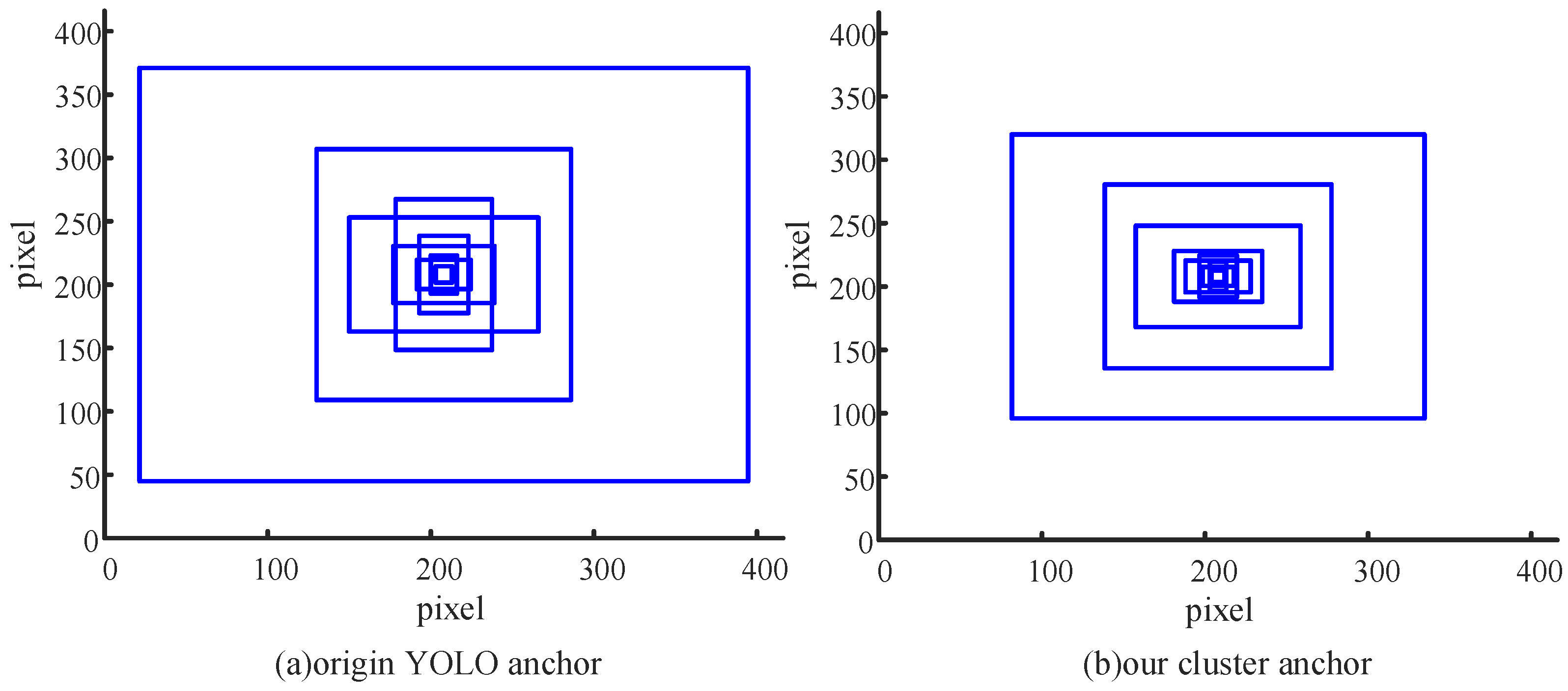
In this paper, after running the clustering algorithm in dataset UA-DETRAC-LITE-NEW multiple times, an optimal group of anchors is obtained: (8,9), (10,23), (19,15), (23,33), (40,25), (54,40), (101,80), (139,145), (253,224). The comparison between the anchor set by the original YOLO algorithm and the anchor with optimal performance obtained by our clustering method in the vehicle detection environment is shown in Figure 4. In this paper, the input image sizes for all target detections are set at 416 × 416, so the comparison in the diagram below is also based on the comparison of original image size. In addition, nine anchors are drawn, with the center of the image (i.e., coordinate position (208,208)) as the center. Through comparison, it can be found that the original YOLO algorithm focuses more on the generality of algorithm, different sizes of anchors have uniform distribution in number, and the algorithm emphasizes universality; the anchors obtained with our clustering algorithm are generally smaller than the anchors obtained with the original YOLO algorithm, and most anchors have small sizes. This also suits the intelligent streetlight environment of IoV. Most vehicles in the image have small sizes.
After completing the anchor data clustering, when there is prior box information closer to the real target, the YOLO algorithm can return to the target position with less iterations, which can reduce the model training times to a certain extent.
3.3. Improvement of the Model’s Generalization Ability
The model’s generalization ability refers to whether the model can have good performance when facing unknown data. We train the model to make the model extract and learn the characteristics of real object, so that the model can be used for real unknown data in the future. From this perspective, the model’s generalization ability is particularly important. On the one hand, mixup is used in target detection in this section to improve model’s generalization ability when facing unknown data (test dataset), thus further improving the model’s average precision; on the other hand, the label smoothing method is introduced in this section to reduce the model’s “confidence” about objects, thus improving the model’s generalization ability.
3.3.1. Improvement Based on Label Smoothing
The training dataset used in this paper is generally from dataset UA-DETRAC. Dataset UA-DETRAC was collected from real roads, while the vehicles on the roads are generally sedans and SUVs, and the number of trucks, pick-ups and commercial vehicles is significantly smaller than that of sedans. Although some of these vehicles, in small numbers, were also manually collected and labeled in this paper, which are also added to the training dataset, this still cannot balance the numbers of various classes of vehicles. For vehicle classes with small numbers in the dataset, the deep neutral network might not be able to learn features with strong generalization ability, and, as a result, the final model obtained by training has poor generalization ability. In this paper, the label smoothing technique is adopted to maximally prevent the problem of the weak generalization ability of the model.
When the target detection algorithm proposed in this paper is finally used to predict the target class, the one-hot coding method is adopted. For example, if the sample is observed as belonging to a certain class, the position of the corresponding class of vector has the value of 1, or otherwise, it is 0. Such a coding method may cause over-fitting when the above samples have uneven distribution, because limited samples are used for training in general, which cannot cover all possible situations. In an extreme example, when the training data include 200,000 sedans but only 3000 pick-ups, the occurrence probability of a sedan is around 98.52%, while that of a pick-up is only about 1.48%. In this case, with continuous training, the neutral network tends to predict the class of sedan, and the probability of the predicted class being a sedan is 100% or very close to 100%, while the class of pick-ups is ignored. At this time, the model is “overconfident” in the prediction of sedans.
The Label Smoothing Regularization (LSR) method aims to alleviate the over-fitting problem which tends to occur because the true-value label is not “soft” enough. It is a constraint method which adds some noise to the true value of the class to constrain the model and lower the over-fitting degree of the trained model.
The LSR formula is as shown in Formula (8), in which represents the one-hot coding after smoothing; , is a small hyper-parameter, which represents the smoothing degree or how much noise has been added to the real value, and bigger indicates more noise has been added to real value; K refers to the number of classes; the true value of the class is generally stored in the ID of the class before being transformed to the one-hot code, and in the formula, y is the ID of the classes true value.
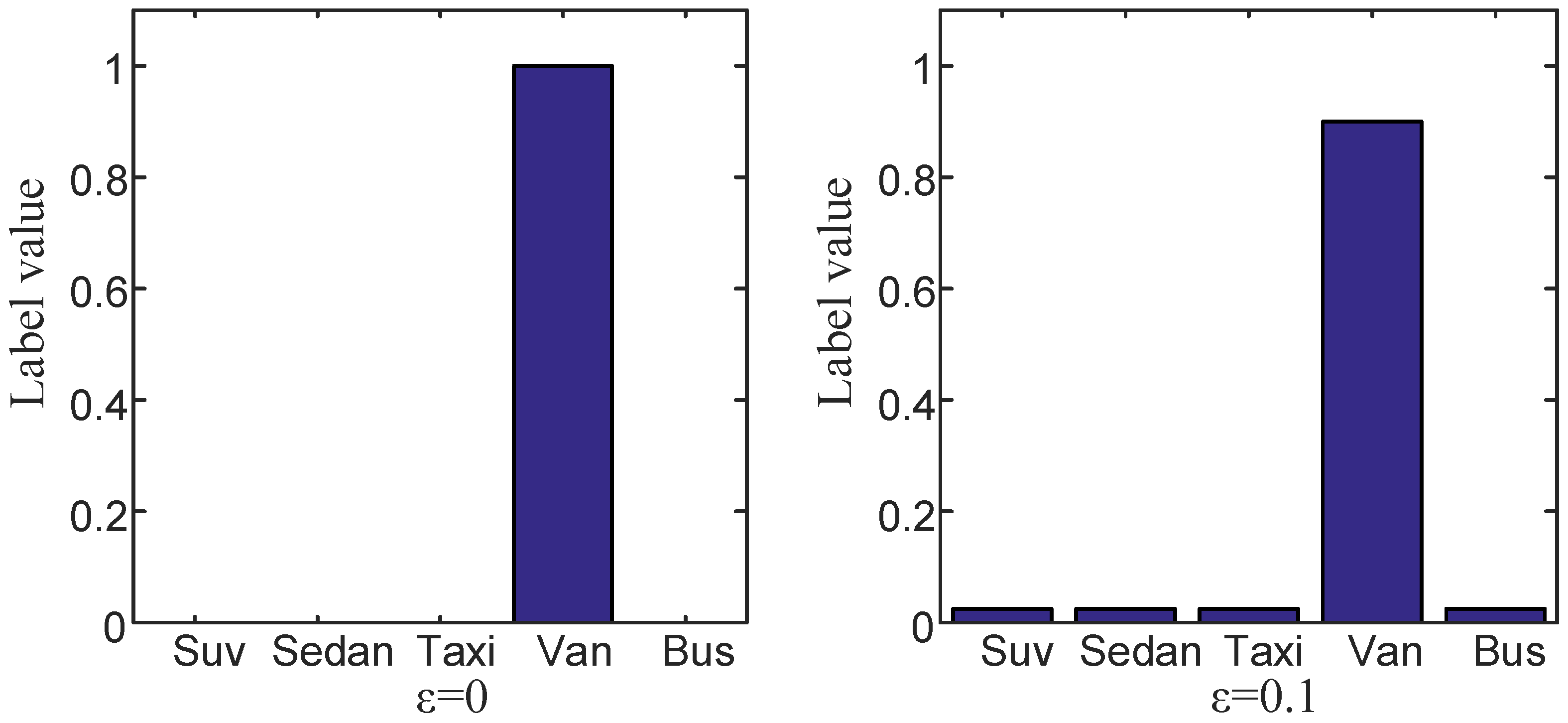
In essence, LSR takes the value of true-value class in the original one-hot code from , and then evenly distributes it among other classes, so that the final distribution of true-value label is no longer distributed on its true-value position. As shown in Figure 5, on the left diagram, which means no LSR; the right diagram shows the case of .
In the above diagram, only five classes are chosen to present the change of label value before and after label smoothing. In the meantime, is set as 0.1 to make it easier to see the change. In practical training, is set as 0.01. It can be seen that the label value has a broader distribution after label smoothing. As a result, the model is finally not that “confident”, and the model’s generalization ability is improved.
3.3.2. Improvement Based on Mixup
In the field of target detection, the data enhancement technique will frequently be used. When the dataset does not contain particularly sufficient data, the deep model is unable to learn good features. In addition, in most datasets, various types of samples are not balanced in number, which will result in poor ability of the model in predicting samples with small numbers. The above problem can be alleviated through data enhancement, which can efficiently improve the network’s performance and generalization ability. Data enhancement refers to utilizing certain image conversion methods (such as random cropping, random translation, angle rotation, mirror image flipping, etc.) based on existing datasets to generate some “new data” for the neural network.
Hongyi Zhang et al. proposed the mixup method, which can be used to effectively improve the performance and generalization ability of the object classification model [20]. The mixup method is a data enhancement method irrelevant to data, which is also simple. It is used to generate new samples with the method shown in Formulas (9) and (10).
The original author applied mixup in the classification task, in which xi and xj are two random image samples, while yi and yj are their corresponding class labels. λ ∈ (0,1), and λ follow a Beta distribution: λ ∈ Beta (α,α), α ∈ (0,∞). The mixup method linearly integrates existing samples and generates new samples, which makes the model more stable.
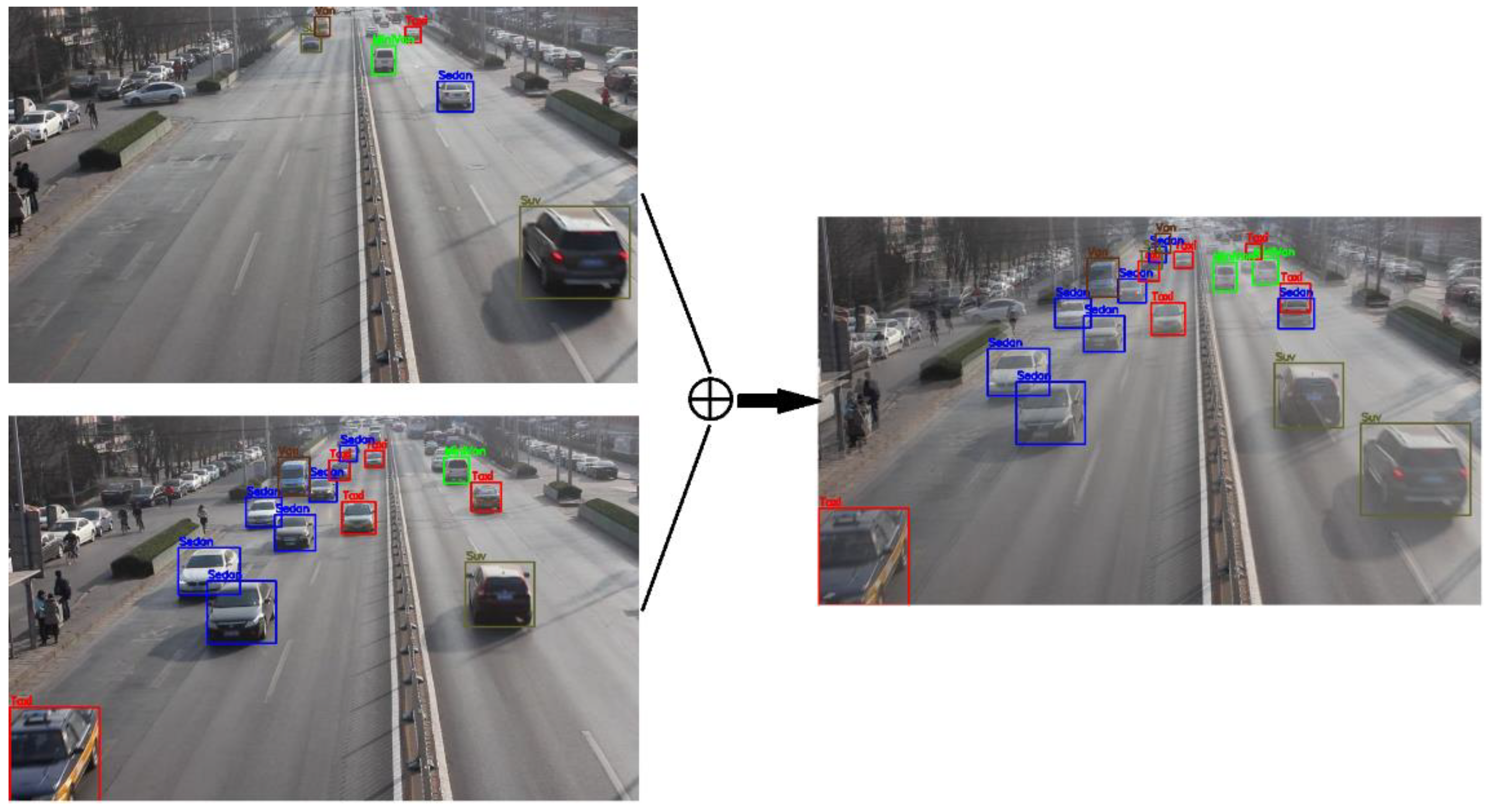
In this paper, the data enhancement technique of mixup is introduced into vehicle target detection. In the dataset used in this paper, all images have 540 × 960 pixels. In image integration, similar to the above Formulas (9) and (10), a new sample x can be obtained through superposition of the corresponding pixels of randomly selected images xi and xj according to linear coefficients λ and (1 − λ). Tags yi and yj of images xi and xj are kept, and tag y is obtained corresponding to a new sample x. A schematic diagram of using mixup to realize data enhancement in the vehicle target detection problem is shown in Figure 6.
3.4. Improvement Based on the Position Regression Loss Function
In the YOLOv3 algorithm, the predicted position (x,y,w,h) of a bounding box is obtained through direct regression, because one bounding box is regressed, while the bounding box may have big size or small size. During calculation of position loss, if the size of the bounding box is not considered, it will cause inaccurate regression of the bounding box, slow training and convergence speed and other problems. YOLOv3 uses the scale factor to reduce the difference in position loss between bounding boxes of different sizes. However, because the L2 distance does not possess scale invariability, this approach will only reduce part of the difference between big and small bounding boxes in loss. Therefore, we believe a distance evaluation index with scale invariability is needed to improve the loss function. In this section, IoU and GIOU will be used as the indices to measure the distance between bounding boxes and improve the loss function of YOLOv3.
3.4.1. Improvement of Loss Function Based on IoU
Because IoU has invariability with the change of scale, it means it is not affected by the sizes of two objects. Therefore, in this section, IoU will be used to improve the loss function of the YOLO algorithm. Moran Ju [21] once proposed using this method to improve the algorithm’s performance, and we adopt this method in our system.
IoU is within the range of 0~1. When IoU is 0, it means the two bounding boxes are completely disjoint; when IoU is 1, it indicates the two bounding boxes completely overlap. Therefore, Formula (11) can be used to describe the distance between two bounding boxes, and this distance can be directly used in the position loss function of the YOLO algorithm.
IoU satisfies scale invariability, which is not affected by the scales of two objects, and it can also be used to describe the distance between two objects. During regression of coordinates, YOLOv3 can use Formula (11) as the distance to directly describe the difference between the predicted bounding box and the real-value bounding box. The size of this difference can be used in the position regression loss function and participate into the network optimization.
3.4.2. Improvement of Loss Function Based on GIOU
IoU has scale invariability and can be used as the index to measure the distance between objects; however, when IoU is used as distance, if the two objects are completely disjoint, no matter whether they are far from or close to each other, the distance value is fixed, which is 1. At this time, the gradient cannot be returned, and the model may be unable to learn the position of part of true-value bounding box during training, which has lowered the final precision of the model. In this section, GIOU will be used as the distance to improve the YOLO position loss.
GIOU is a new index used to measure the overlapping degree between two bounding boxes on the basis of IoU, which considers the non-overlapping area not considered by IoU, and it can reflect the overlapping method between A and B. Assume the coordinate of the predicted bounding box is , and the coordinate of true-value bounding box is . GIOU and the computation process using GIOU as the loss function is as follows:
- (1)
- In order to ensure the coordinates of the predicted box satisfy and , conduct data manipulation as in Formulas (12)–(15):
- (2)
- Calculate the area of :
- (3)
- Calculate the area of :
- (4)
- Calculate the intersection between and :
- (5)
- Find the smallest rectangular box enclosing and :
- (6)
- Calculate the area of :
- (7)
- Calculate IoU and GIOU:
- (8)
- Obtain the loss function based on GIOU:
4. Experiment and Results
4.1. Evaluation Metrics
In this paper, we adopt the broadly used evaluation model indices with concentrated VOC data: average precision (AP) and mean average precision (mAP). In addition, the parameters of confusion matrix, PR curve, model frames per second (FPS), etc. are also used to further evaluate the model.
See Formulas (30) and (31) for the calculation of AP and mAP.
where represents the curve function with precision (P) as the ordinate and recall (R) as the abscissa, hereafter referred to as the PR curve. The enclosed area by the PR curve and abscissa axis is AP; mAP refers to the mean average precision, which equals to the sum of the precisions of all classes divided by the class number N. In this paper, the 11-point computation method in VOC2007 is used for calculation of precision.
The indices of precision and recall were mentioned above, and, in order to introduce these two indices, we need to introduce other common indices. In general, the multi-classification task can be split into multiple binary classification tasks, and, in binary classification, the samples are generally divided into positive samples and negative samples. Therefore, for real value and predicted value, the following four situations may occur through combination: the true value is a positive sample, and the predicted value is also a positive sample, which is called true positive (TP); the true value is a positive sample, while the predicted value is a negative sample, which is called false negative (FN); the true value is a negative sample, while the predicted value is a positive sample, which is called false positive (FP); the true value is a negative sample, and the predicted value is also a negative sample, which is called true negative (TN). However, in a target detection task, the target is regarded as a positive sample, and the background is treated as a negative sample, so the background will not be detected in target detection task. Therefore, the two indices of TN and FN are generally not used. In this paper, indices which can better reflect the model performance will be built based on TP and FP.
See Formula (32) for the definition of precision; in general, see Formula (33) for the definition of recall. However, in the abovementioned target detection problem, FN and TN are generally not discussed. TP+FN refers to the number of positive samples, and the number of positive samples can be obtained from the true-value tag. Therefore, in this paper, Formula (34) is used to redefine recall, and it is not different from the original definition in meaning. In it, refers to the number of positive samples; see Formula (35) for the definition of measurement.
The confusion matrix is another index used to evaluate the model performance. Its row vector represents the true value, and its column vector represents the predicted value. Therefore, it is easy and intuitive to find which class is misclassified into another class from the confusion matrix. In addition, the frames per second (FPS) can also be used to measure the computation efficiency of algorithm.
4.2. Experimental Results
4.2.1. Improved Experimental Results Based on Results of Scale Optimization
In this section, dataset UA-DETRAC-LITE-NEW is used to conduct an experiment with the original YOLOv3 algorithm and the algorithm proposed in this section, respectively. In the experiment, the following data are preprocessed: randomly regulate the brightness, contrast, hue and saturation; by ensuring that there is bounding box, randomly crop the image; randomly turn the image; conduct other operations. During training, set the batch size at 4, and in order to realize faster convergence of the network, conduct continuous training based on the trained pre-training weight by the author of YOLOv3 on ImageNet. Use the gradient descent method with momentum to optimize the model. Set the momentum as 0.9 and the learning rate as 0.001.
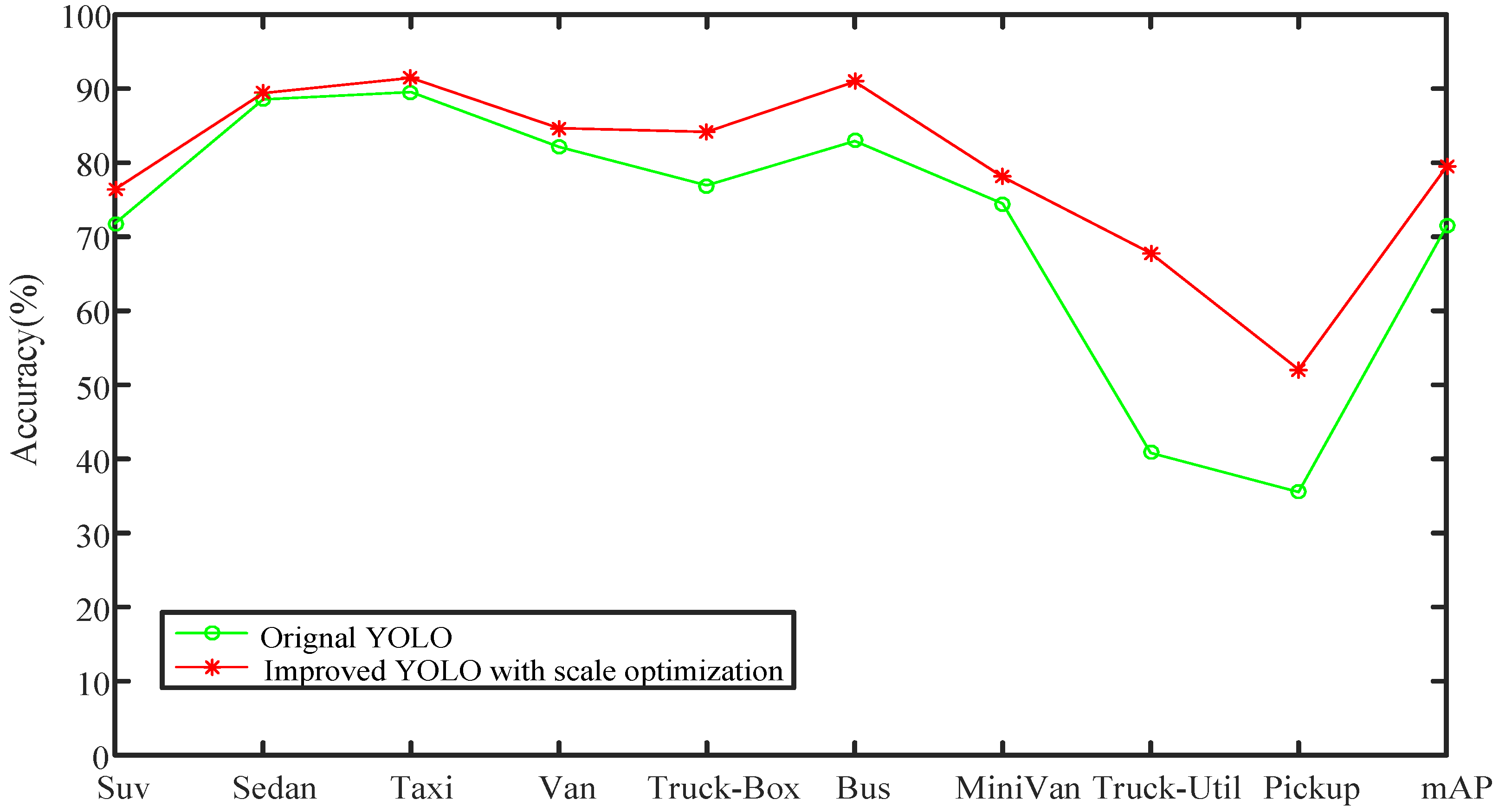
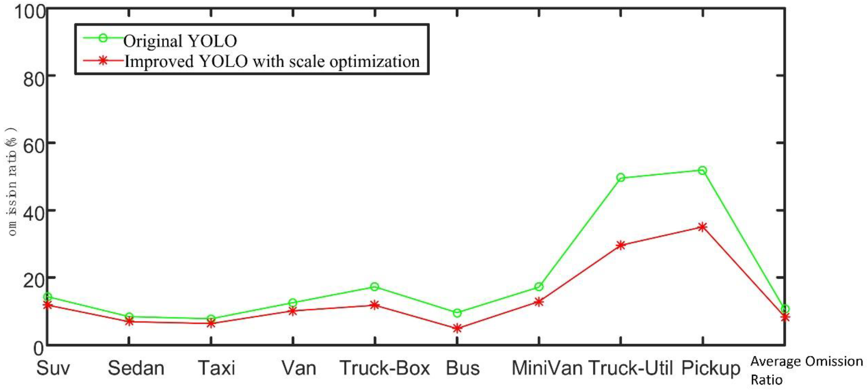
The average precision (AP) of each class and the mean average precision (mAP) of all classes are obtained in the experiment. See Table 1 for specific data; a more intuitive diagram comparison is shown in Figure 7. The comparison diagram of the omission ratio is presented in Figure 8; the confusion matrix is shown in Table 2.
According to the experimental results, it can be seen that the improved YOLO algorithm proposed in this section can significantly improve the detection performance for the two classes of trucks and pick-ups. In precision, the detection precisions for the classes of trucks and pick-ups are increased by 26.98% and 16.54%, respectively; through further analysis of the omission ratio, it can be seen that the main reason for the low precisions of the two classes of trucks and pick-ups is that they have low omission ratios, which further lowers the index of precision.
Although the detection precisions for trucks and pick-ups are significantly increased after improvement, their precisions are still lower than the average level. Next, the improved model proposed in this section will be continuously analyzed through confusion matrix. The row vector of confusion matrix represents the true value, while the column vector represents the predicted value. Therefore, the confusion matrix can only be used to analyze the distribution and accuracy of detected targets by the model. The diagonal from upper left to lower right represents the prediction accuracy for detected targets, and other positions indicate false class detections of detected targets. Through the confusion matrix, it can be seen that the detection accuracies for trucks and pick-ups by the improved model in this section are not low, so we can conclude that the main cause for the low precisions for these two classes is that they involve high omission ratios. Through the confusion matrix, we can also see that the model predicts the class of SUVs with true value of 9.36% as sedans and predicts pick-ups with a value of 8.33% as sedans. This indicates that the model has not learned more specific features of SUVs and pick-ups yet.
By comparing the omission ratios of different algorithms, we can find that, after clustering, the model has a lower omission ratio. This can also be summed up as follows: after anchor clustering, the prior information of size closer to the size of real target is provided to the model, so that the model can regress more target positions faster, and the detection rate is increased accordingly.
4.2.2. Improved Experimental Results Based on Improving Model’s Generalization Ability
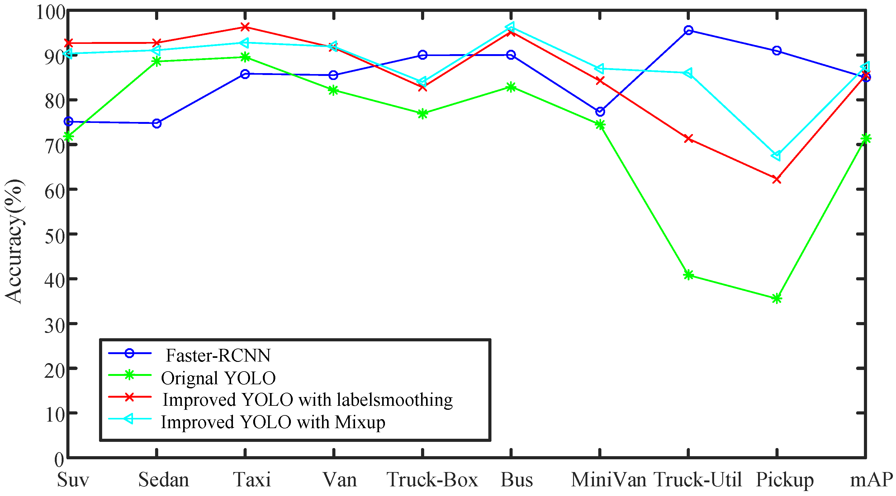
In the experiments of this section, the classic two-stage target detection algorithm Faster-RCNN is used as the algorithm for comparison with the original YOLO algorithm and the improved YOLO algorithm proposed in this section. Among them, the Faster-RCNN algorithm adopts ResNet50 with stronger feature extraction ability as its backbone network. The improved algorithm 1 in this section requires the following experimental conditions: the anchor of the original YOLO algorithm, multi-scale training, using label smoothing, and using mixup for the first 10 epochs of training. The improved algorithm 2 in this section requires the following experimental conditions: the anchor for clustering of vehicle detection scenario in this paper, multi-scale training, using label smoothing, and using mixup for the first 10 epochs of training.
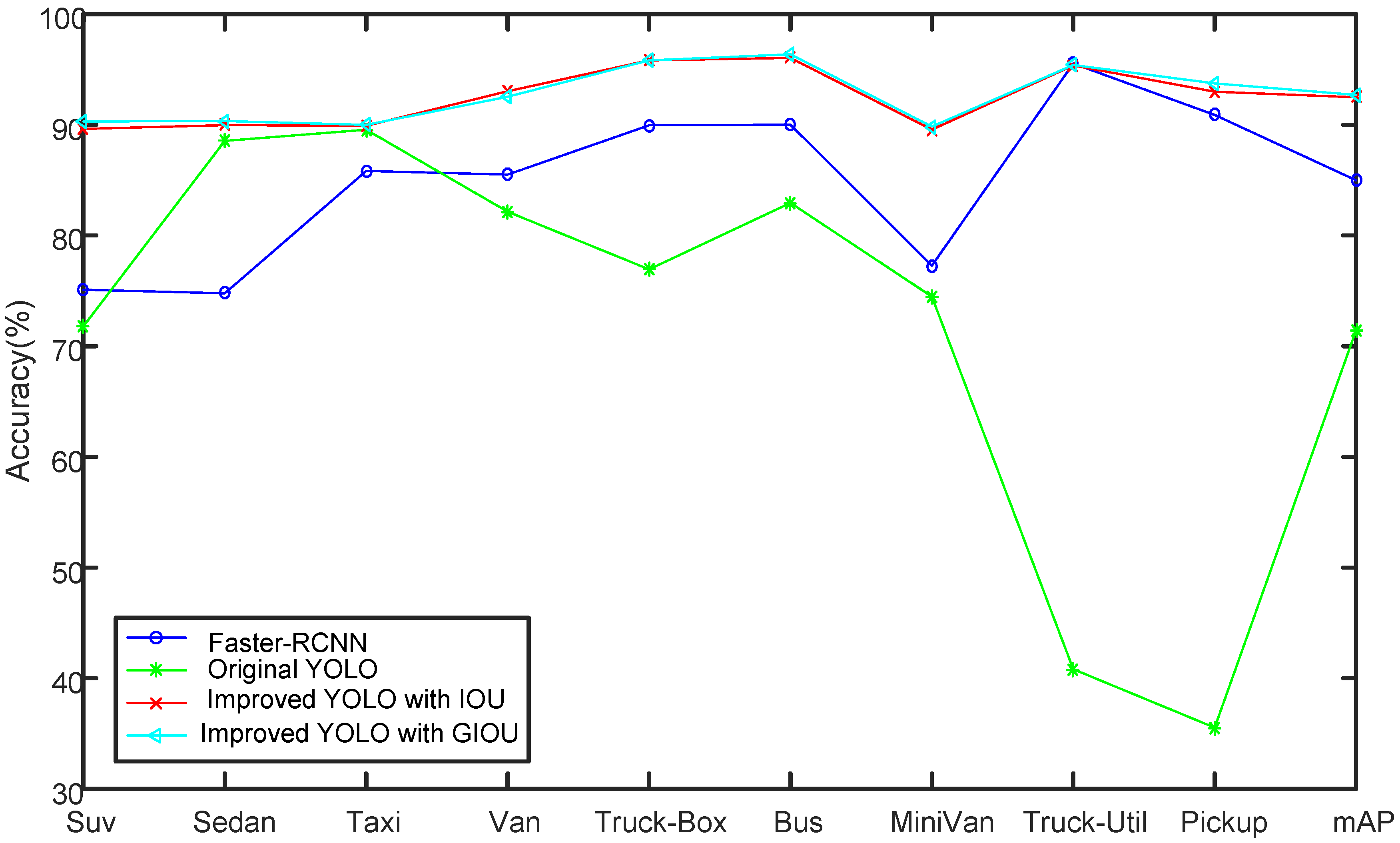
According to Table 3 and Figure 9, it can be seen that the various precisions of the two-stage Faster-RCNN algorithm are higher than the precisions of the YOLO algorithm. This is because Faster-RCNN adopts the RPN network to generate candidate area that may contain the target, so that more candidate areas can be obtained, and the reliability is also higher. Therefore, the Faster-RCNN algorithm has low omission ratio, and its precision is improved as a result. In addition, because dataset UA-DETRAC-LITE-NEW has labeled many pick-ups captured by camera from a long distance, where it is almost impossible to see the back of pick-up with human eyes, it is difficult to detect the class of the pick-up. By comparing the performances of the Faster-RCNN algorithm, the original YOLO algorithm, the improved YOLO algorithm 1 and the improved YOLO algorithm 2 in this section, it can be seen that the mixup and label smoothing methods can be used to effectively improve the model’s generalization ability, almost without increasing the network computation overhead, so as to further improve the model’s accuracy.
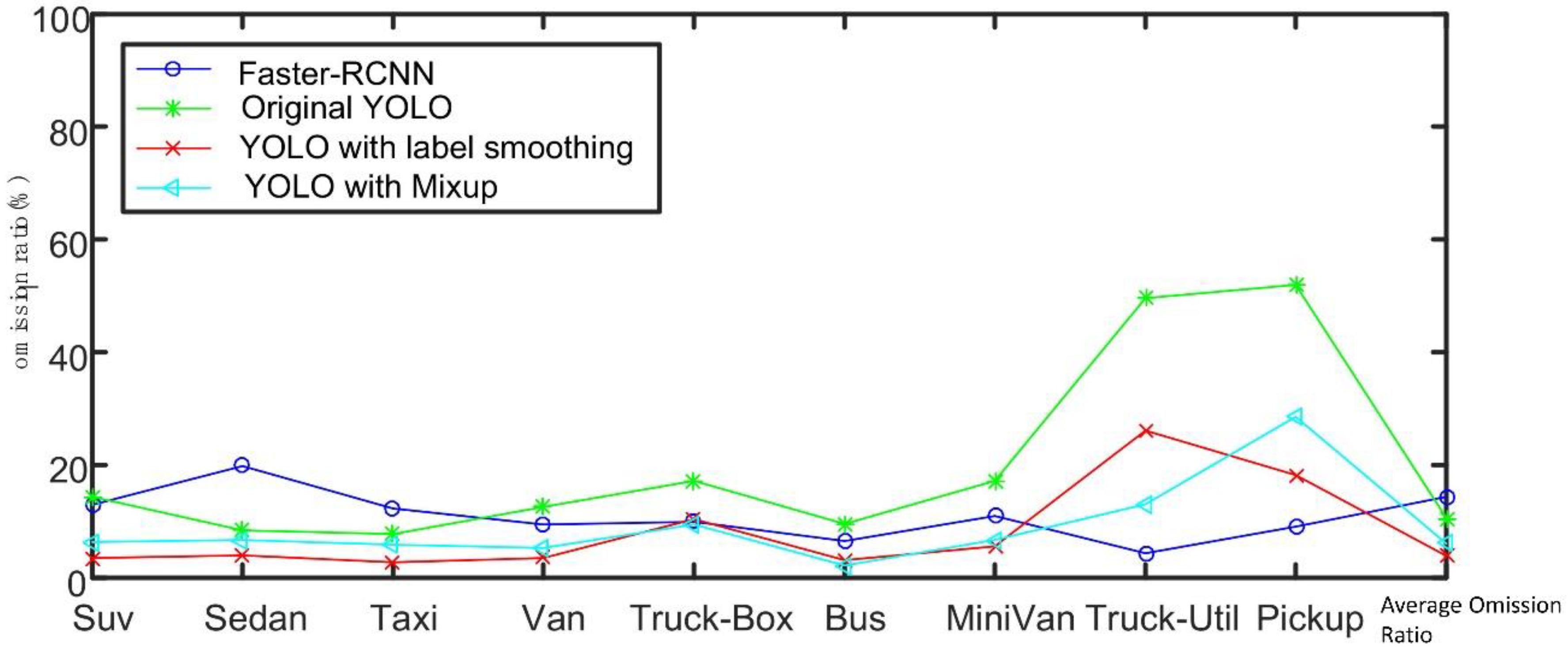
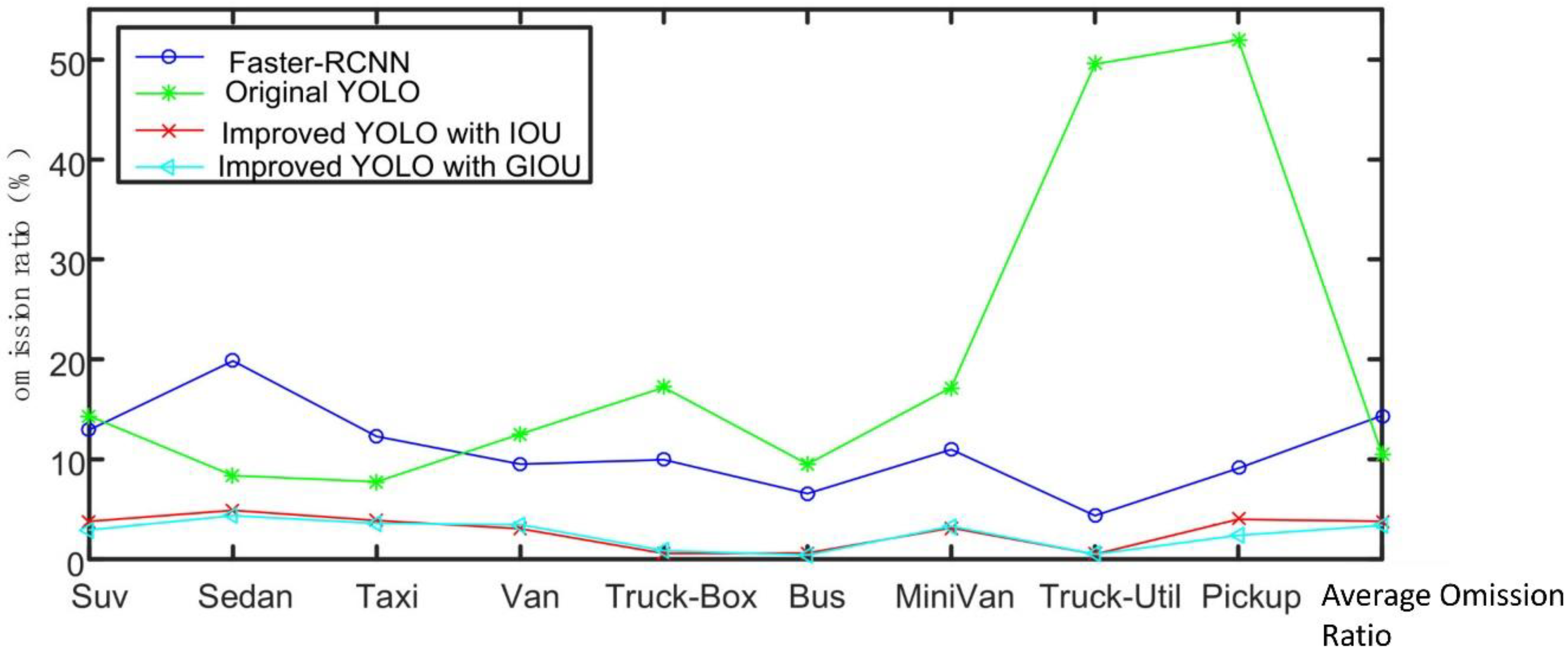
According to Figure 10, it can be seen that the improved YOLO algorithms have lower omission ratios. Although the improved algorithm 2 has a higher omission ratio than the improved algorithm 1 in general, similar to the situation in the previous section, because the improved algorithm involves a higher FP ratio, the improved algorithm 2 has a higher average precision than the improved algorithm 1. Furthermore, the average omission ratio of the two improved algorithms is lower than that of the Faster-RCNN algorithm for comparison, and their omission ratio for most classes is lower than that of Faster-RCNN. Their omission ratio is higher than that of Faster-RCNN only for the two classes of pick-ups and trucks, which once more proves the effectiveness of the improved algorithm.
Table 4 shows the improved YOLO confusion matrix in this section. According to analysis of the confusion matrix, the probability of the model misclassifying the detected target into another class is very small. For the class of small commercial vehicles, the model falsely predicts 3.58% of small commercial vehicles as SUVs, and this is probably because the small commercial vehicles are close to SUV in height and size. In contrast, the model also falsely predicts 0.8% of SUVs as small commercial vehicles.
The main difference between improved algorithm 1 and improved algorithm 2 in this section is whether the anchor for clustering of the vehicle detection scenario proposed in this paper is used. It can be seen that when the anchor obtained through clustering is used to train the model, the performance can be improved by 1.98% compared to the performance of the improved algorithm using the original anchor. Once again, it proves that the model performance can be effectively improved for scenario clustering.
4.2.3. Improved Experimental Results Based on IoU Loss
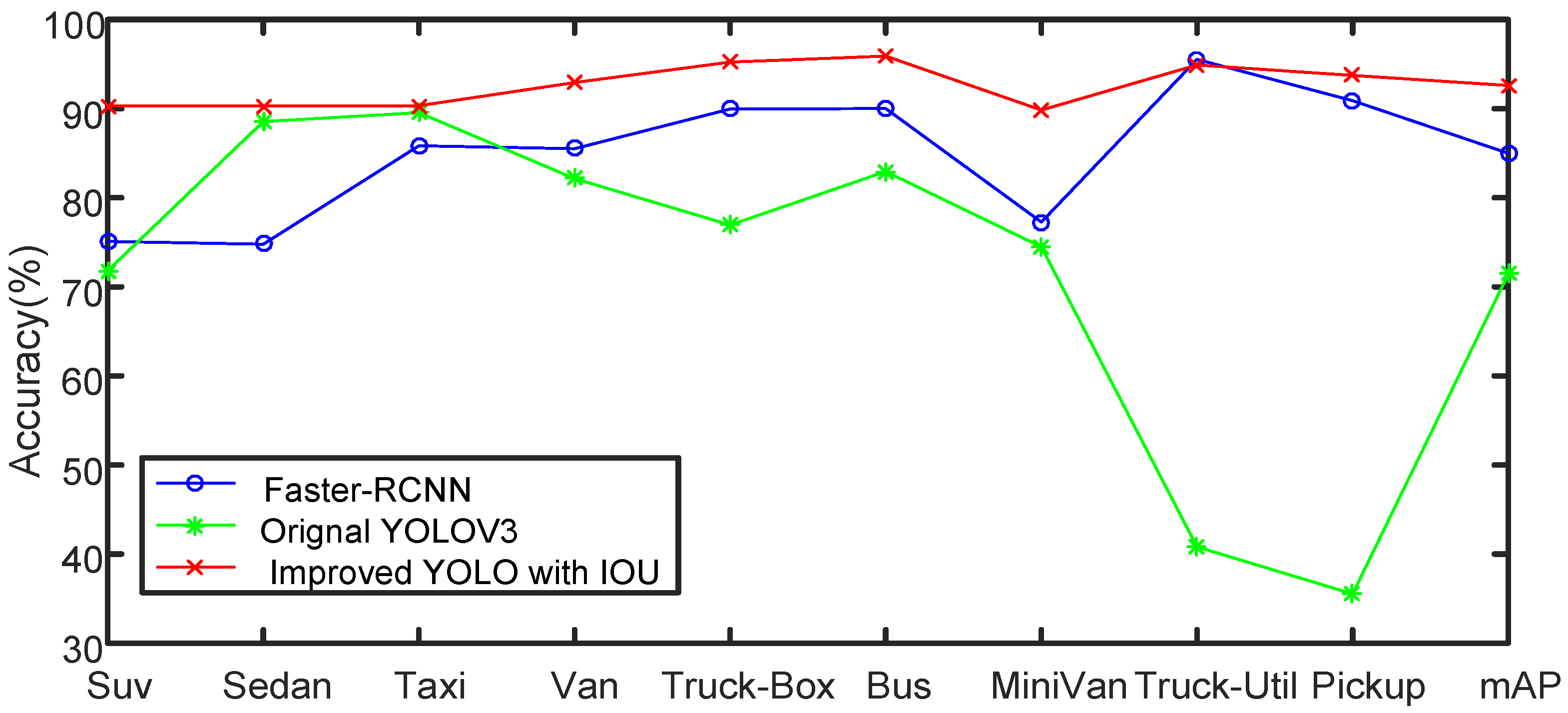
In this section, we will verify the effects of replacing the original L2 loss with IoU loss in the position regression loss. The improved algorithm in this section involves the following experimental conditions: the anchor for clustering of the vehicle detection scenario described in this paper, multi-scale training, using label smoothing, and using mixup for the first 10 epochs of training. The situation of the loss function is as follows: using the IoU loss as position loss, using the L2 norm loss function as confidence loss, and using cross entropy as class loss.
According to Table 5 and Figure 11, when the position regression loss function is modified as the IoU loss function, the model performance is significantly improved. Except for trucks, its precision in predicting the other classes is higher than that of Faster-RCNN with high precision. The YOLOv3 algorithm has two main shortages: firstly, this algorithm is not very accurate in regression of object position; secondly, it has a low recall rate. For the problem of inaccurate regression of object position, the IoU loss in this section is irrelevant to scale, which can reduce the influence of different scales and improve the model’s performance.
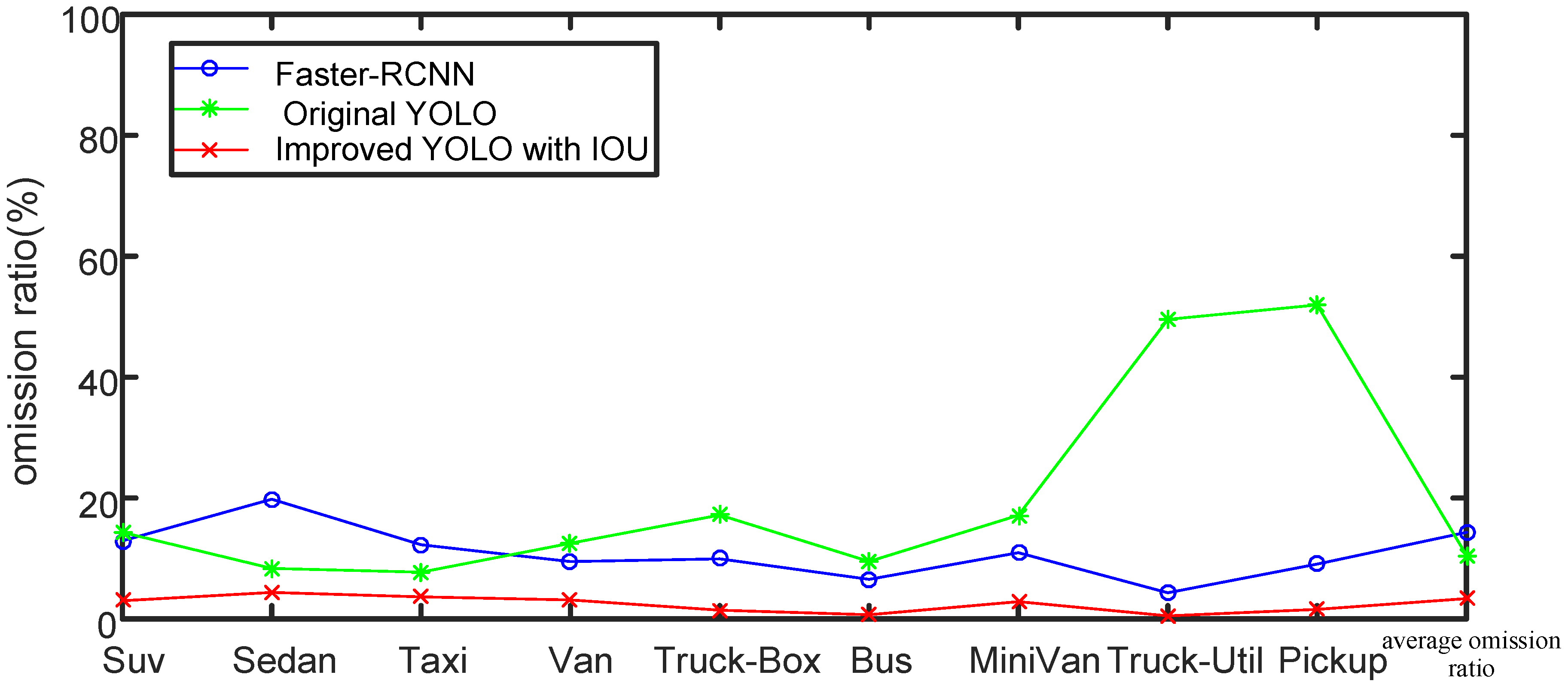
In Figure 12, we compare the omission ratio and average omission ratio for each class of object. It can be seen that, after employing the IoU loss function, the omission ratio is lower than that of the original algorithm and the other algorithm in comparison. The output end of the YOLOv3 algorithm will predict 10,647 bounding boxes; some of these 10,647 bounding boxes will be filtered through the confidence threshold value, and the rest of the bounding boxes will continue to participate in the operation of the NMS algorithm. In the NMS algorithm, there is a threshold value of IoU. If the IoU of the selected bounding box and surrounding bonding boxes is higher than the threshold value, the surrounding bounding boxes will be deleted. From this perspective, if the model has predicted the correct target, but the location of predicted target is not very accurate, then this predicted target might be deleted in the NMS process due to inaccurate location, which will reduce the model’s precision. According to the above result, it can be seen that, after using the IoU loss, the precision is improved, the omission rate is reduced, and the model performance is further improved.
4.2.4. Improved Experimental Results Based on GIOU Loss
In this section, we will verify the effects of replacing the original L2 loss with GIOU loss in the position regression loss. The improved algorithm 1 in this section requires the following experimental conditions: the anchor for clustering of the vehicle detection scenario described in this paper, multi-scale training, not using label smoothing, and using mixup for the first 10 epochs of training. The loss function is as follows: using the GIOU loss as position loss, using the L2 norm loss function as confidence loss, and using cross entropy as class loss. The improved algorithm 2 in this section requires the following experimental conditions: the anchor for clustering of the vehicle detection scenario described in this paper, multi-scale training, using label smoothing, and using mixup for the first 10 epochs of training. The loss function is as follows: using the GIOU loss as position loss, using the L2 norm loss function as confidence loss, and using cross entropy as class loss.
As shown in Table 6 and Figure 13, the two improved algorithms have very similar performance. The average precision of improved algorithm 2 is 0.22% higher than that of improved algorithm 1. They also have very close performance in precision for each class, and the difference is that the improved algorithm 1 does not use label smoothing, while the improved algorithm 2 uses it. According to the experimental results in this section, it can be seen that GIOU can also be used as the position regression loss function to well optimize the model.
As shown in Figure 14, similar to the comparison in terms of precision, the omission ratio of improved algorithms in this section is significantly lower than that of the Faster-RCNN algorithm and the original YOLO algorithm.
To sum it up, we believe that GIOU and IoU can be used as the position loss function to well regress the target position, accelerate the model’s convergence speed, reduce the training volume of the model and improve the final performance of the model.
5. Conclusions
In this article, we propose a distributed system based on smart streetlights, build the dataset UA-DETRAC-LITE-NEW, and improve the YOLOv3 algorithm in various respects. On the intelligent streetlight platform, we have realized fine-grained automobile detection for SUVs, sedans, taxis, commercial vehicles, small commercial vehicles, vans, buses, trucks and pick-ups; we have conducted scale optimization for the vehicle target and improved the model by introducing multi-scale training and anchor clustering; as a result, the detection accuracies for trucks and pick-ups are improved by 26.98% and 16.54%, respectively, and average accuracy is increased by 8%. The label smoothing and mixup methods are used to improve the model’s generalization ability, and its generalization ability is increased by 16.01% compared to the original YOLO algorithm. By combining the position regression loss function of IOU or GIOU for optimization, the system accuracy can reach 92.7%, which is 21.28% higher than that of the original YOLOv3 algorithm. For further development, we can continue to optimize the YOLOv3 algorithm from the perspective of confidence loss.
Author Contributions
F.Y. proposed the idea of this article and finished the manuscript. Z.H. led the research project. D.Y. finished the code and performed the experiment. Y.F. performed experimental results analysis. K.J. participated in the experiment. All authors have read and agreed to the published version of the manuscript.
Funding
This work is supported by the Sichuan Province Science and Technology Program Research Project (No.2019YJ0174).
Conflicts of Interest
The authors declare no conflict of interest.
References
- Zhu, L.; Yu, F.R.; Wang, Y.; Ning, B.; Tang, T. Big Data Analytics in Intelligent Transportation Systems: A Survey. IEEE Trans. Intell. Transp. Syst. 2019, 20, 383–398. [Google Scholar] [CrossRef]
- Maddio, S. A Compact Circularly Polarized Antenna for 5.8-GHz Intelligent Transportation System. Antennas Wirel. Propag. Lett. 2017, 16, 533–536. [Google Scholar] [CrossRef]
- Herrera-Quintero, L.F.; Vega-Alfonso, J.C.; Banse, K.B.A.; Carrillo Zambrano, E. Smart ITS Sensor for the Transportation Planning Based on IoT Approaches Using Serverless and Microservices Architecture. IEEE Intell. Transp. Syst. Mag. 2018, 10, 17–27. [Google Scholar] [CrossRef]
- Ferreira, D.L.; Nunes, B.A.A.; Obraczka, K. Scale-Free Properties of Human Mobility and Applications to Intelligent Transportation Systems. IEEE Trans. Intell. Transp. Syst. 2018, 19, 3736–3748. [Google Scholar] [CrossRef]
- Girshick, R.; Donahue, J.; Darrell, T.; Malik, J. Rich Feature Hierarchies for Accurate Object Detection and Semantic Segmentation. In Proceedings of the 2014 IEEE Conference on Computer Vision and Pattern Recognition, Columbus, OH, USA, 23–28 June 2014; pp. 580–587. [Google Scholar]
- Liu, W.; Anguelov, D.; Erhan, D.; Szegedy, C.; Reed, S.; Fu, C.-Y.; Berg, A.C. SSD: Single Shot MultiBox Detector. arXiv 2016, arXiv:1512.02325. [Google Scholar]
- Simonyan, K.; Zisserman, A. Very Deep Convolutional Networks for Large-Scale Image Recognition. arXiv 2015, arXiv:1409.1556. [Google Scholar]
- Redmon, J.; Divvala, S.; Girshick, R.; Farhadi, A. You Only Look Once: Unified, Real-Time Object Detection. In Proceedings of the 2016 IEEE Conference on Computer Vision and Pattern Recognition (CVPR), Las Vegas, NV, USA, 27–30 June 2016; pp. 779–788. [Google Scholar]
- Chu, W.; Liu, Y.; Shen, C.; Cai, D.; Hua, X.-S. Multi-Task Vehicle Detection With Region-of-Interest Voting. IEEE Trans. Image Process. 2018, 27, 432–441. [Google Scholar] [CrossRef] [PubMed]
- Geiger, A.; Lenz, P.; Urtasun, R. Are we ready for autonomous driving? The KITTI vision benchmark suite. In Proceedings of the 2012 IEEE Conference on Computer Vision and Pattern Recognition, Providence, RI, USA, 16–21 June 2012; pp. 3354–3361. [Google Scholar]
- Everingham, M.; Van Gool, L.; Williams, C.K.I.; Winn, J.; Zisserman, A. The Pascal Visual Object Classes (VOC) Challenge. Int. J. Comput. Vis. 2010, 88, 303–338. [Google Scholar] [CrossRef] [Green Version]
- Cao, C.-Y.; Zheng, J.-C.; Huang, Y.-Q.; Liu, J.; Yang, C.-F. Investigation of a Promoted You Only Look Once Algorithm and Its Application in Traffic Flow Monitoring. Appl. Sci. 2019, 9, 3619. [Google Scholar] [CrossRef] [Green Version]
- Lyu, S.; Chang, M.-C.; Du, D.; Li, W.; Wei, Y.; Del Coco, M.; Carcagnì, P.; Schumann, A.; Munjal, B.; Choi, D.-H.; et al. UA-DETRAC 2018: Report of AVSS2018 & IWT4S challenge on advanced traffic monitoring. In Proceedings of the 2018 15th IEEE International Conference on Advanced Video and Signal Based Surveillance (AVSS), Auckland, New Zealand, 27–30 November 2018; pp. 1–6. [Google Scholar]
- Wen, L.; Du, D.; Cai, Z.; Lei, Z.; Chang, M.-C.; Qi, H.; Lim, J.; Yang, M.-H.; Lyu, S. UA-DETRAC: A New Benchmark and Protocol for Multi-Object Detection and Tracking. Comput. Vis. Image Underst. 2020, 193, 102907. [Google Scholar] [CrossRef] [Green Version]
- Lyu, S.; Chang, M.-C.; Du, D.; Wen, L.; Qi, H.; Li, Y.; Wei, Y.; Ke, L.; Hu, T.; Del Coco, M.; et al. UA-DETRAC 2017: Report of AVSS2017 & IWT4S Challenge on Advanced Traffic Monitoring. In Proceedings of the Advanced Video and Signal Based Surveillance (AVSS), Lecce, Italy, 29 August–1 September 2017; pp. 1–7. [Google Scholar]
- Geiger, A.; Lenz, P.; Stiller, C.; Urtasun, R. Vision meets robotics: The kitti dataset. Int. J. Robot. Res. 2013, 32, 1231–1237. [Google Scholar] [CrossRef] [Green Version]
- Redmon, J.; Farhadi, A. YOLOv3: An Incremental Improvement. arXiv 2018, arXiv:1804.02767. [Google Scholar]
- He, K.; Zhang, X.; Ren, S.; Sun, J. Deep Residual Learning for Image Recognition. In Proceedings of the 2016 IEEE Conference on Computer Vision and Pattern Recognition (CVPR), Las Vegas, NV, USA, 27–30 June 2016; pp. 770–778. [Google Scholar]
- Lin, T.-Y.; Dollar, P.; Girshick, R.; He, K.; Hariharan, B.; Belongie, S. Feature Pyramid Networks for Object Detection. In Proceedings of the 2017 IEEE Conference on Computer Vision and Pattern Recognition (CVPR), Honolulu, HI, USA, 21–26 July 2017; pp. 936–944. [Google Scholar]
- Zhang, H.; Cisse, M.; Dauphin, Y.N.; Lopez-Paz, D. mixup: Beyond Empirical Risk Minimization. arXiv 2018, arXiv:1710.09412. [Google Scholar]
- Ju, M.; Luo, H.; Wang, Z.; Hui, B.; Chang, Z. The Application of Improved YOLO V3 in Multi-Scale Target Detection. Appl. Sci. 2019, 9, 3775. [Google Scholar] [CrossRef] [Green Version]
Figure 1.
Smart streetlights in the Internet of Vehicles.

Figure 2.
Labelling of vehicles with image label software.

Figure 3.
Images of dataset UA-DETRAC.

Figure 4.
Comparison of anchor before and after clustering.

Figure 5.
Schematic diagram of Label Smoothing Regularization.

Figure 6.
Schematic diagram of Mixup.

Figure 7.
Comparison of accuracy between the original YOLO algorithm and its improved algorithm.

Figure 8.
Comparison of omission ratio between the original YOLO algorithm and its improved algorithm.
Figure 8.
Comparison of omission ratio between the original YOLO algorithm and its improved algorithm.

Figure 9.
Comparison of Faster-RCNN, YOLO and improved YOLO in terms of precision.

Figure 10.
Comparison of Faster-RCNN, YOLO and improved YOLO in terms of omission ratio.

Figure 11.
Comparison of Faster-RCNN, original YOLO and improved YOLO algorithm with IoU loss function in terms of precision.
Figure 11.
Comparison of Faster-RCNN, original YOLO and improved YOLO algorithm with IoU loss function in terms of precision.

Figure 12.
Comparison of Faster-RCNN, original YOLO and improved YOLO algorithm with IoU loss function in terms of omission ratio.
Figure 12.
Comparison of Faster-RCNN, original YOLO and improved YOLO algorithm with IoU loss function in terms of omission ratio.

Figure 13.
Comparison of Faster-RCNN, original YOLO and improved YOLO algorithm with GIoU loss function in terms of precision.
Figure 13.
Comparison of Faster-RCNN, original YOLO and improved YOLO algorithm with GIoU loss function in terms of precision.

Figure 14.
Comparison of Faster-RCNN, original YOLO and improved YOLO algorithm with GIOU loss function in terms of omission ratio.
Figure 14.
Comparison of Faster-RCNN, original YOLO and improved YOLO algorithm with GIOU loss function in terms of omission ratio.


Table 1.
Comparison of accuracy between the original YOLO algorithm and its improved algorithm.
| Type | Original YOLO (%) | YOLO with Scale Optimization (%) |
|---|---|---|
| Suv | 71.80 | 76.42 |
| Sedan | 88.55 | 89.41 |
| Taxi | 89.55 | 91.45 |
| Van | 82.15 | 84.67 |
| Truck-Box | 76.94 | 84.16 |
| Bus | 82.94 | 90.94 |
| MiniVan | 74.48 | 78.08 |
| Truck-Util | 40.82 | 67.80 |
| Pickup | 35.54 | 52.08 |
| mAP | 71.42 | 79.45 |
Table 2.
The confusion matrix of the improved YOLO algorithm (unit %).
| Type | Suv | Sedan | Taxi | Van | Truck-Box | Bus | MiniVan | Truck-Util | Pickup |
|---|---|---|---|---|---|---|---|---|---|
| Suv | 88.35 | 9.36 | 0.25 | 0.17 | 0 | 0 | 1.87 | 0 | 0 |
| Sedan | 0.21 | 99.48 | 0.22 | 0.05 | 0 | 0 | 0.05 | 0 | 0 |
| Taxi | 0 | 0.42 | 99.52 | 0 | 0 | 0 | 0.05 | 0 | 0 |
| Van | 0.45 | 0.57 | 0.11 | 95.69 | 0 | 0 | 3.17 | 0 | 0 |
| Truck-Box | 0 | 1.55 | 0 | 1.55 | 96.37 | 0 | 0 | 0.52 | 0 |
| Bus | 0 | 0.17 | 0 | 0 | 0 | 99.83 | 0 | 0 | 0 |
| MiniVan | 1.94 | 2.53 | 0.17 | 1.6 | 0 | 0 | 93.76 | 0 | 0 |
| Truck-Util | 0 | 0 | 0 | 1.27 | 0 | 0 | 0 | 98.73 | 0 |
| Pickup | 0 | 8.33 | 0 | 2.08 | 0 | 0 | 0 | 2.08 | 87.5 |
Table 3.
Comparison of Faster-RCNN, YOLO and improved YOLO in terms of precision.
| Type | Faster-RCNN (%) | Original YOLO (%) | Label Smoothing (%) | Mixup (%) |
|---|---|---|---|---|
| Suv | 75.10 | 71.80 | 92.66 | 90.33 |
| Sedan | 74.78 | 88.55 | 92.72 | 91.08 |
| Taxi | 85.83 | 89.55 | 96.27 | 92.79 |
| Van | 85.50 | 82.15 | 91.63 | 91.88 |
| Truck-Box | 89.95 | 76.94 | 82.78 | 83.98 |
| Bus | 90.01 | 82.94 | 95.19 | 96.25 |
| MiniVan | 77.27 | 74.48 | 84.25 | 86.98 |
| Truck-Util | 95.53 | 40.82 | 71.30 | 86.02 |
| Pickup | 90.89 | 35.54 | 62.34 | 67.53 |
| mAP | 84.99 | 71.42 | 85.46 | 87.43 |
Table 4.
Improved YOLO confusion matrix in this section (unit %).
| Type | Suv | Sedan | Taxi | Van | Truck-Box | Bus | MiniVan | Truck-Util | Pickup |
|---|---|---|---|---|---|---|---|---|---|
| Suv | 98.35 | 1.57 | 0 | 0 | 0 | 0 | 0.8 | 0 | 0 |
| Sedan | 0.23 | 99.7 | 0.2 | 0.2 | 0.3 | 0 | 0 | 0 | |
| Taxi | 0.5 | 0.21 | 99.68 | 0 | 0 | 00 | 0.5 | 0 | 00 |
| Van | 0.43 | 1.18 | 0 | 97.33 | 0 | 0 | 1.7 | 0 | 0 |
| Truck-Box | 0 | 0.53 | 0 | 0 | 98.41 | 0 | 0 | 1.6 | 0 |
| Bus | 0 | 0 | 0 | 0 | 0 | 1 | 0 | 0 | 0 |
| MiniVan | 3.58 | 0.7 | 0 | 0.62 | 0 | 0 | 95.9 | 0 | 0 |
| Truck-Util | 0 | 0 | 0 | 0 | 0 | 0 | 0 | 1 | 0 |
| Pickup | 0 | 0 | 0 | 1.85 | 0 | 0 | 0 | 1.85 | 96.3 |
Table 5.
Comparison of Faster-RCNN, original YOLO and improved YOLO algorithm with IoU loss function in terms of precision.
Table 5.
Comparison of Faster-RCNN, original YOLO and improved YOLO algorithm with IoU loss function in terms of precision.
| Type | Faster-RCNN (%) | Original YOLO (%) | Improved YOLO with IoU (%) |
|---|---|---|---|
| Suv | 75.10 | 71.80 | 90.29 |
| Sedan | 74.78 | 88.55 | 90.32 |
| Taxi | 85.83 | 89.55 | 90.32 |
| Van | 85.50 | 82.15 | 92.92 |
| Truck-Box | 89.95 | 76.94 | 95.23 |
| Bus | 90.01 | 82.94 | 95.90 |
| MiniVan | 77.27 | 74.48 | 89.84 |
| Truck-Util | 95.53 | 40.82 | 94.89 |
| Pickup | 90.89 | 35.54 | 93.73 |
| mAP | 84.99 | 71.42 | 92.60 |
Table 6.
Comparison of Faster-RCNN, original YOLO and improved YOLO algorithm with GIOU loss function in terms of precision.
Table 6.
Comparison of Faster-RCNN, original YOLO and improved YOLO algorithm with GIOU loss function in terms of precision.
| Type | Faster-RCNN (%) | Original YOLO (%) | Improved YOLO with IoU (%) | Improved YOLO with GIOU (%) |
|---|---|---|---|---|
| Suv | 75.10 | 71.80 | 89.63 | 90.30 |
| Sedan | 74.78 | 88.55 | 89.97 | 90.34 |
| Taxi | 85.83 | 89.55 | 89.91 | 89.99 |
| Van | 85.50 | 82.15 | 93.03 | 92.53 |
| Truck-Box | 89.95 | 76.94 | 95.82 | 95.82 |
| Bus | 90.01 | 82.94 | 96.04 | 96.36 |
| MiniVan | 77.27 | 74.48 | 89.56 | 89.83 |
| Truck-Util | 95.53 | 40.82 | 95.36 | 95.4 |
| Pickup | 90.89 | 35.54 | 92.99 | 93.74 |
| mAP | 84.99 | 71.42 | 92.48 | 92.70 |
© 2020 by the authors. Licensee MDPI, Basel, Switzerland. This article is an open access article distributed under the terms and conditions of the Creative Commons Attribution (CC BY) license (http://creativecommons.org/licenses/by/4.0/).
Share and Cite
MDPI and ACS Style
Yang, F.; Yang, D.; He, Z.; Fu, Y.; Jiang, K. Automobile Fine-Grained Detection Algorithm Based on Multi-Improved YOLOv3 in Smart Streetlights. Algorithms 2020, 13, 114. https://0-doi-org.brum.beds.ac.uk/10.3390/a13050114
AMA Style
Yang F, Yang D, He Z, Fu Y, Jiang K. Automobile Fine-Grained Detection Algorithm Based on Multi-Improved YOLOv3 in Smart Streetlights. Algorithms. 2020; 13(5):114. https://0-doi-org.brum.beds.ac.uk/10.3390/a13050114
Chicago/Turabian StyleYang, Fan, Deming Yang, Zhiming He, Yuanhua Fu, and Kui Jiang. 2020. "Automobile Fine-Grained Detection Algorithm Based on Multi-Improved YOLOv3 in Smart Streetlights" Algorithms 13, no. 5: 114. https://0-doi-org.brum.beds.ac.uk/10.3390/a13050114
Note that from the first issue of 2016, this journal uses article numbers instead of page numbers. See further details here.