Change-Point Detection in Autoregressive Processes via the Cross-Entropy Method


Department of Mathematics and Statistics, Macquarie University, Sydney, NSW 2109, Australia
*
Author to whom correspondence should be addressed.
Algorithms 2020, 13(5), 128; https://0-doi-org.brum.beds.ac.uk/10.3390/a13050128
Submission received: 10 April 2020
/
Revised: 18 May 2020
/
Accepted: 18 May 2020
/
Published: 20 May 2020
Abstract
:It is very often the case that at some moment a time series process abruptly changes its underlying structure and, therefore, it is very important to accurately detect such change-points. In this problem, which is called a change-point (or break-point) detection problem, we need to find a method that divides the original nonstationary time series into a piecewise stationary segments. In this paper, we develop a flexible method to estimate the unknown number and the locations of change-points in autoregressive time series. In order to find the optimal value of a performance function, which is based on the Minimum Description Length principle, we develop a Cross-Entropy algorithm for the combinatorial optimization problem. Our numerical experiments show that the proposed approach is very efficient in detecting multiple change-points when the underlying process has moderate to substantial variations in the mean and the autocorrelation coefficient. We also apply the proposed method to real data of daily AUD/CNY exchange rate series from 2 January 2018 to 24 March 2020.
1. Introduction
Change-point detection in time series processes, or time series segmentation, has been discussed by many authors in the fields of statistics, computer science, and data mining for several decades [1]. Change-point detection has a broad range of applications, including financial time series analysis [2,3], econometrics [4,5], and science and engineering [6,7,8]. Change-point problems are traditionally divided into two large categories: posterior (off-line) and sequential (on-line) problems; see, for example, [9]. The former is often referred to as segmentation of a signal or time series when all data are observed, while the latter assumes a stream of data coming in real-time. In this paper, we focus on the time series segmentation problem.
A change-point is defined when at least one statistical parameter in a given time series process suddenly changes, which may be caused by the variation in the mean, trend, or other internal parameters. Following the assumption of [10] and [7], a non-stationary time series process is assumed to be segmented by change-points into a sequence of piecewise stationary processes. We are interested in modeling the non-stationary autoregressive AR (p) process and estimating the unknown number of segments and the locations of change points.
Various algorithms have been proposed in time series segmentation with the aim of searching for the optimal solutions based on different types of objective (or score) functions. There are two main streams of widely used optimization methods; one is related to the Binary segmentation [11,12,13,14], and the other method is based on the dynamic programming algorithm [15,16,17]. In addition, several well-known computational approaches have been applied to change-point problems. These include the EM algorithm [18], the genetic algorithm [19,20], sequential importance sampling [21,22], MCMC algorithms [23,24,25], hybrid algorithms [26,27,28,29], and the Cross-Entropy method [8,30,31,32,33,34,35].
Many of the existing multiple change-point methods assume independence of observations. Because of this assumption, these methods tend to either underestimate or overestimate the number of change-points in autoregressive time series due to its endogenous dependent structure. For example, a stationary AR(1) process with moderate to strong autocorrelation can be confused with a change-point process with independent observations causing these segmentation methods to overestimate the number of structural breaks. References [7] and [36] took the dependence structure of autoregressive time series into account and developed a segmentation method to identify break-points using a genetic algorithm and a dynamic programming algorithm, respectively, with the objective function based on the minimum description length (MDL) information criterion. Another paper [4] implemented a strucchange algorithm designed for estimating structural changes in linear regression. Recently, [37] proposed a AR1seg approach for estimating change-points in the AR(1) model based on the assumption of a common autocorrelation coefficient for all segments. In this paper, we apply the Cross-Entropy (CE) method with the MDL principle to identify the number of and locations of change-points. In contrast to [35], we assume that observations from different segments may be generated from different AR() processes. The statistical features, such as the order of autoregressive processes, the autocorrelation parameter, and the mean of the homogeneous segment, can be estimated if the change-points are detected, but our focus is on the detection accuracy of identifying change-points. Through extensive numerical experiments, our method shows superior detection accuracy when the underlying autocorrelation structure changes.
The paper is organized as follows. Section 2 introduces the MDL-based objective function and compares it with other popular model selection criteria, and the detailed derivation is provided. In Section 3, we describe the proposed algorithm in detail. Section 4 shows the design and results of numerical experiments. Real data analysis is shown in Section 5. Lastly, Section 6 provides a general discussion.
2. Model Selection Criteria
2.1. Change-Point Detection Problem
Firstly, let us formulate the change-point detection problem. Let denote a data sequence of length T. Assume there are N unknown change-points, so X is segmented into segments by the set of locations , , where the i-th segment consists of observations ; i is numbered from 1 to . Next, we assume that the data sequence X is generated by piecewise stationary AR() processes, the model assumes that the observations within each segment are generated by a stationary AR() process with autocorrelation coefficients , mean , and variance . The segments are assumed to be independent of each other. The parameters , , and are not known in advance, whereas is known.
where the noise , , , and the model allows for shifts in the mean, ; also define , . It is necessary to specify the unknown parameter N, the number of change-points. Theoretically, N could be any integer between 0 and , while in practice, we can set a maximum value for N, perhaps via the rough graphical inspection. Additionally, the change-point problem is characterized by N; if N is greater than 1, we call it multiple change-point problem; otherwise, the process is stationary. A model selection procedure is often used to determine the number of change-points; one can minimize an objective function of the form [38]:
where the is a cost function for a segment and is a penalty term. In this paper, we consider the negative log-likelihood as the cost function by rewriting (2) as a penalized likelihood information criterion:
Akaike’s information criterion (AIC), Bayesian information criterion (BIC), and modified BIC are well-known information criteria. The significant difference between these information criteria is the amount of penalty added to each parameter of the model. The penalty terms for the AIC and the BIC are given below:
The total number of parameters in the model is denoted by k. Thus, each parameter is penalized by the same amount. Because the AIC and BIC are not theoretically designed for the change-point problems, Zhang and Siegmund [39] proposed the modified BIC (mBIC) for determining the number of change-points in array-based comparative genomic hybridization data. The mBIC follows the classic BIC, while it differs in the penalty term. The general form that penalizes for model dimensions is given:
In addition, Lavielle [40] proposed a penalty function with an adjustable shrinkage parameter for the change-point problem:
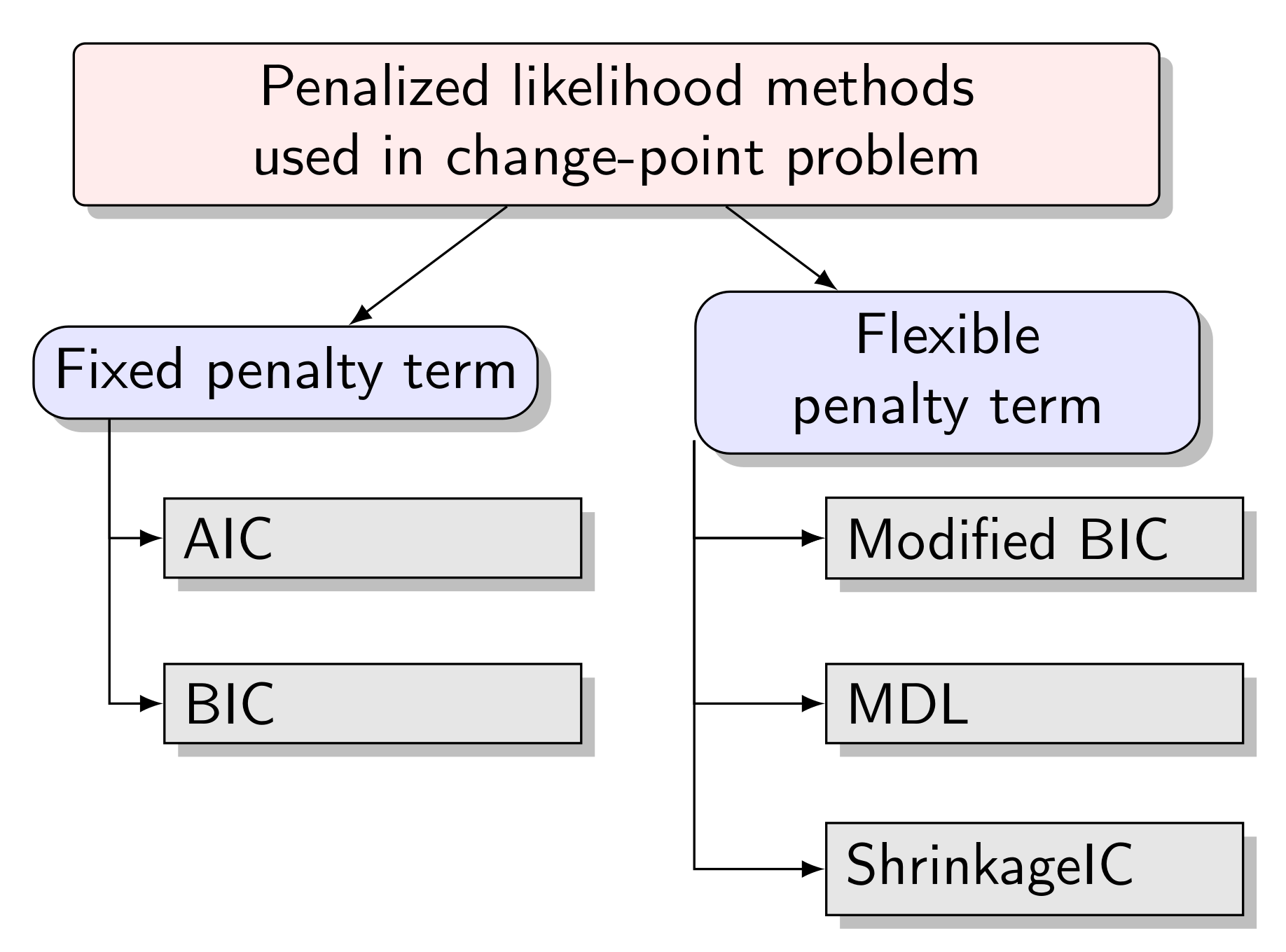
In this paper, we introduce the two-stage minimum description length (MDL) for our change-point problem based on model (1); the superior flexibility is one strength of MDL. It was proposed by Rissanen (1978), based on Kolmogorov’s theory of algorithmic complexity and rooted in information theory. In developing MDL, Rissanen’s idea was to select the model with an excellent fit to the observed data while generating the least description. The term “description length” is interchangeable with “code length,” which is used to describe the complexity of each statistical model. In other words, the best model was defined by MDL as the one that can compress a vast amount of information by using less computer memory storage; the amount of computer memory is called code length, denoted by . Figure 1 summarizes the aforementioned penalized likelihood methods.
2.2. The Principle of Minimum Description Length
The MDL criterion can tailor penalties for parameters having different natures, while the other information criteria treat every parameter as imposing the same penalty; therefore, which parameter to be penalized and the amount to be encoded need to be formalized according to the general principles of Rissanen [41]:
- For an integer parameter N, when its value is not bounded, approximately bits are encoded. If N is limited by the upper bound value , then approximately bits are needed.
- To encode a real parameter, if it is estimated from T observations, bits are required.
Then, we use the framework set out by [7] to derive the description length based on model (1); the MDL consists of the following four components:
- As mentioned above, the first part of two-stage MDL can be considered as a negative log-likelihood function of the whole process, by assuming that the segments are independent, and using the approximation in McLeod et al. [42] for the exact loglikelihood for the AR(p) model, the likelihood of segment i can be written as (see [42] for further details), where is the Yule-Walker estimate, is the covariance determinant of first s observations.
- For the number N, the penalty term is . Since it can be considered as an integer parameter without being bounded, the code length is .
- The length for each of segments cannot exceed T. This means that, according to the integer parameter principle, the lengths of the segments can be encoded with bits.
- represents the order of the AR process for each segment, which should be an integer. So the parameter can be encoded with bits; see [7].
- For each segment i, , we estimate three real-valued parameters. These are mean shift ; autocorrelation coefficient , where ; and variance . Under the real parameter principle, each of these parameters can be computed from observations. Hence, each of them need bits.
Thus, we can get the objective functions based on the MDL for the multiple change-points model:
If there are no change-points in the model (), the MDL for a stationary AR(p) process will be
3. The Cross-Entropy Algorithm
In order to identify the locations of change-points in the problem—Equations (8) and (9), which can be considered a combinatorial optimization problem—we use the cross-entropy (CE) algorithm. The CE method was originally developed to estimate the rare-event probabilities as an adaptive importance sampling method, based on the Kullback–Leibler divergence (or cross-entropy) minimization [43]. The main idea of the CE method can be described by a two-step iterative procedure:
- Generate a sample from a probability distribution.
- In order to obtain a better sample, find the minimum cross-entropy distance between the sample distribution and a target distribution.
Rubinstein [44,45] then realized that the CE method can be used to solve combinatorial optimization problems. We recommend [46] for getting familiar with the principals and the applications of the CE method.
Firstly, we formulate the rare-event probability estimation problem:
where is the objective (or score) function defined on a finite set , is a threshold, is the corresponding probability measure when C follows the probability density function (pdf) with a real parameter v, and I is an indicator function. The main idea of the CE method is to obtain the optimal pdf from a set of pdfs through minimizing Kullback–Leibler (or relative entropy) distance.
It allows us to generate a sequence by multi-level CE implementation to get the final optimal pdf . During adaptive updating procedure, a family of is generated and eventually converges to the optimal state .
Then, the two-step iterative procedure mentioned above can be written in the following way:
- Updating of the level parameter . Order the performance score increasingly, , . Let be the -quantile of the ordered performance scores, which can be denoted as,
- Updating the reference parameter . Given and , we can derive from Equation (10),
More formally, the generic CE optimization algorithm can be described as follows (Algorithm 1).
| Algorithm 1 Basic CE optimization algorithm. |
|
The detailed information about the properties of the CE algorithm as well as its diverse applications can be found in [43] and [44]. To date, the CE method has been modified and applied to different multiple change-point problems as a combinatorial optimization algorithm in [8,30,31,32,33,34,35].
Let us now formulate the CE algorithm for the multiple change-point problem. Let be a sequence representing the locations of change-points. Since the location space is finite, we can carry out the CE combinatorial optimization algorithm, and generate M rows of random samples. So here we deal with the objects , . The external parameters are , , and ; we apply the CE.AR algorithm at . The normal distribution is served as . In practice, the users need to specify the external parameters. The main steps of our proposed CE.AR algorithm are as follows (Algorithm 2).
| Algorithm 2 The CE.AR algorithm. |
|
4. Numerical Experiments
We provide three simulated examples to illustrate the proposed CE.AR method, compared with the current methods on offer in the R packages AR1seg [37] and strucchange [47]. In the simulation study, we aim to present a detailed evaluation of the estimated number of change-points through these three methods. The CE algorithm discussed above was implemented using the breakpoint package [8] with the external settings as follows: the elite proportion value and the sample size .
4.1. Example 1: Simulated AR(1) Processes with No Change-Point
The null case is considered first with three standard AR(1) processes simulated with no change-point. Three sets of 100 AR(1) sequences are generated with each sequence of length . The autocorrelation coefficients were set to be 0.1, 0.5, and 0.9, respectively, for each set. The variance was set globally to be , and the mean was set to be .
Table 1 shows that both strucchange and CE.AR perform well for all values of , while AR1seg tends to slightly overestimate the number of change-points when the value autocorrelation parameter increases. The best performing method is the CE.AR method.
4.2. Example 2: Simulated AR(1) Processes with a Single Change-Point
In this example, we would like to understand how a change in either the mean or the autocorrelation coefficient affects the performances of the algorithms. To study these individual effects, we design two scenarios. In the first scenario, we assume that autocorrelation remains the same in a time series, while the mean jumps at each segment; the second scenario shows the opposite situation: the mean is fixed and the autocorrelation coefficient varies across segments.
4.2.1. Example 2.1
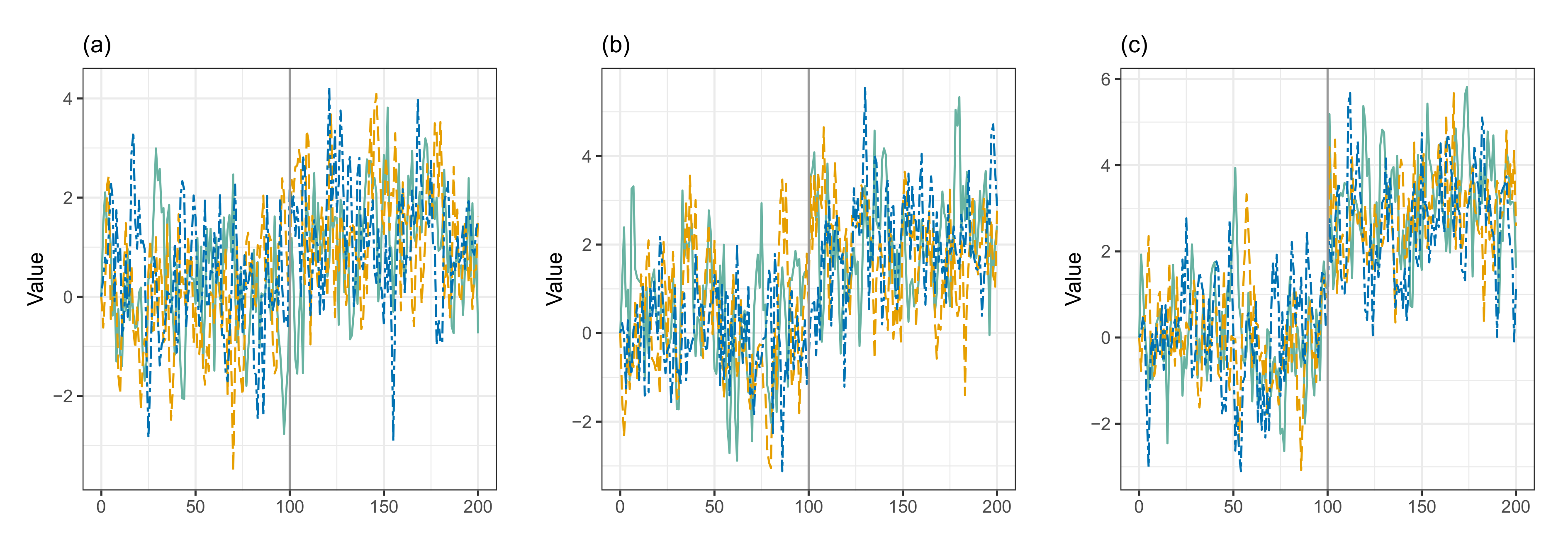
In scenario 1, we generated three sets of 100 AR(1) sequences of length 201 with a fixed autocorrelation and one abrupt change-point at position , which partitions a time series into two segments. The mean of first segment, , equal 0, and then jumps from 0 to or or at the second segment. For each set, three sequences of simulated piecewise AR(1) process are graphically demonstrated by Figure 2.
Table 2 shows that the detection accuracies of all the methods strucchange, AR1seg, and CE.AR improved while the value of increased. Generally, the best performing method was the strucchange package.
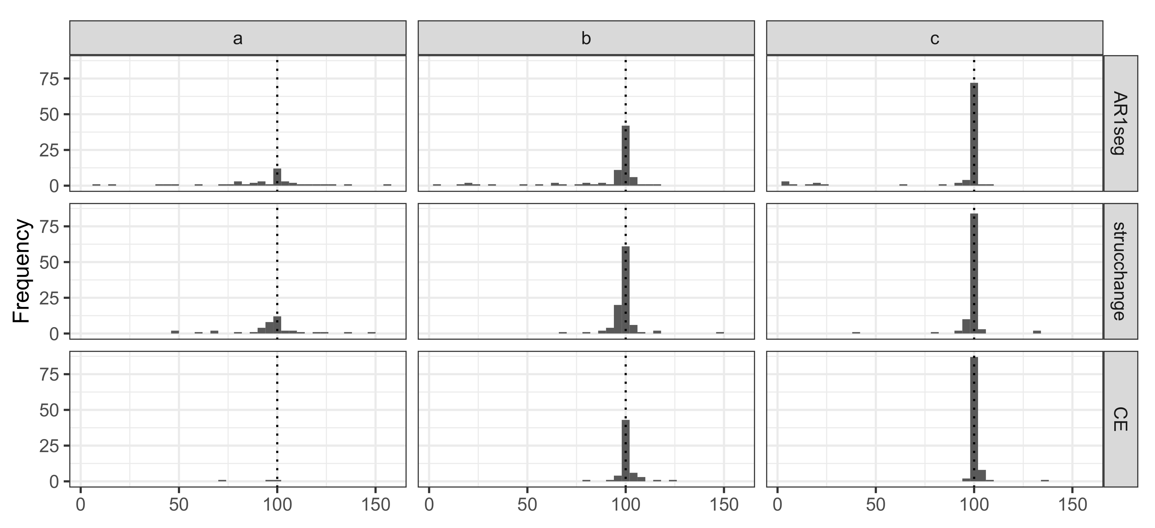
We use the histogram (see Figure 3) to illustrate the performance of the estimated single change-point location under three levels of mean shifts by looking at the plot vertically to compare three methods (a,b,c) under the same settings. Overall, all methods tend to more accurately identify the change-point’s location as the mean shifts become more significant. By examining the case of or 3, we can see that AR1seg identified a few change-points located at the beginning of the process, while the CE.AR method tended to seek locations around 100. Under the case of , all the methods perform poorly; the CE.AR method especially is insensitive to the small mean change.
4.2.2. Example 2.2
In scenario 2, we generated three sets of 100 AR(1) sequences of length 201 with a homogeneous mean and one abrupt change-point at position caused by the variation in autocorrelation coefficient. Three settings are displayed in Table 3; in the first set, a weak positive correlation is followed by a moderate correlation; the change occurs from weak to strong, and from moderate to vigorous, in the second and third sets respectively. In general, the performance of strucchange is relatively better than AR1seg and CE.AR. AR1seg is not explicitly designed for this scenario since the autoregressive parameter changes between segments. It is interesting to see that CE.AR method performs very well only when varies dramatically. When does not change that much, the algorithm tends to underestimate the number of change-points, preferring a model with a smaller number of change-points.
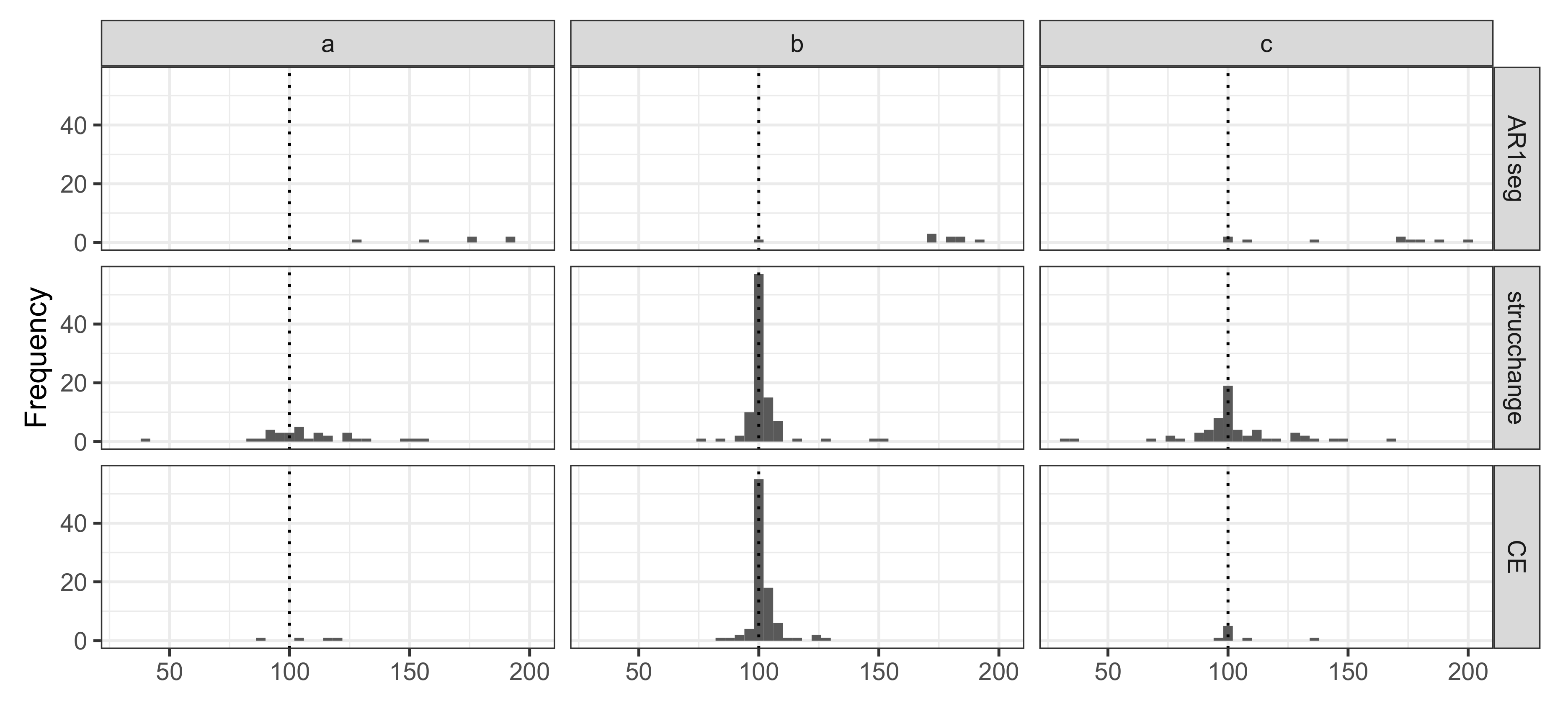
Figure 4 displays that the estimation performance of each method under scenario 2. The strucchange shows better performance than the other two. Compared with scenario 1, when the autoregressive parameter varies weakly or moderately, it is more difficult for the three methods to estimate the correct number of and the locations of change-points. Lastly, the histogram shows that the estimated location of strucchange has a broader spread than CE.AR method.
In addition, we run more tests when changes from negative to positive; three settings are displayed in Table 4. The detection rates of strucchange and CE.AR methods increased in comparison with the previous settings.
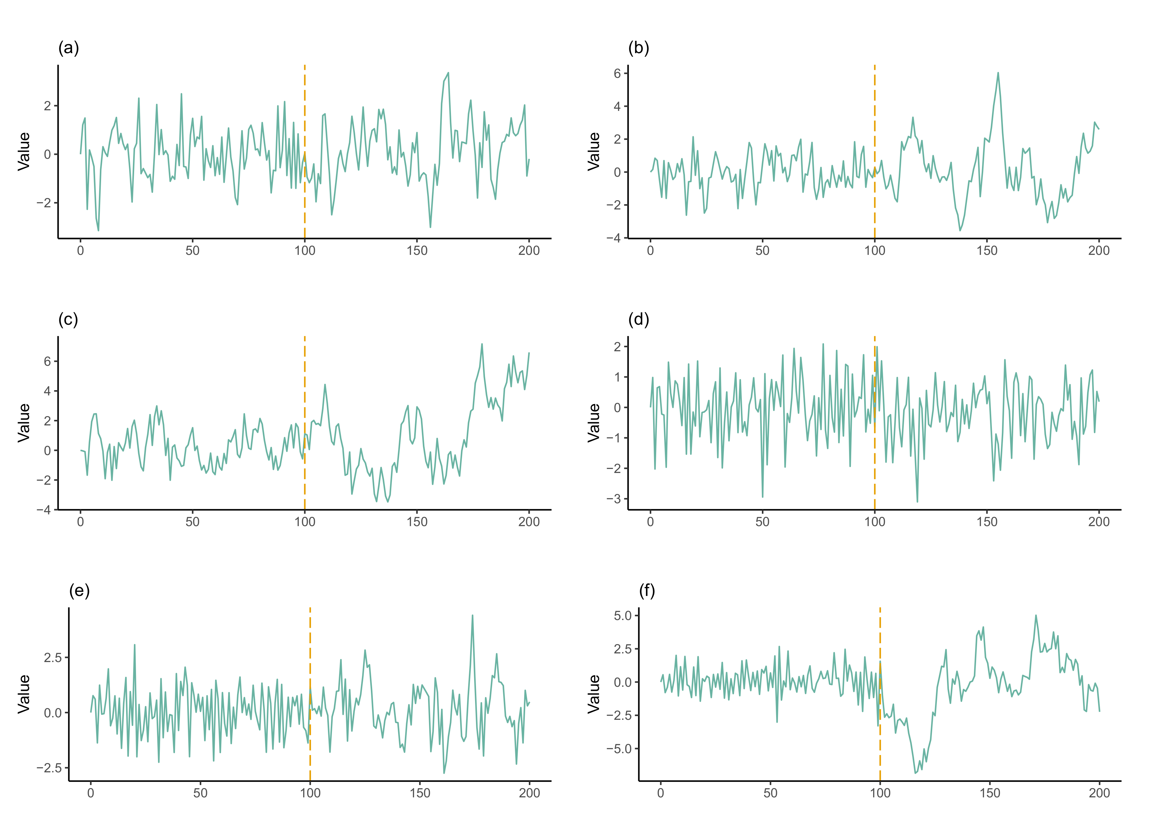
In Example 2, we have considered two scenarios of single change-point detection. The first scenario assumes that there are no coefficient changes while the mean changes between different segments. In the second scenario, the coefficient parameter changes, but the mean is assumed to be 0. Individually, the coefficients are simulated to change weakly, moderately, and strongly; we have considered six cases, which are graphically illustrated in Figure 5 by plotting one time series out of the 100 simulated AR(1) sequences. The frequency charts are used to measure the performances of the three methods in terms of accuracy of estimating the location of the change-point. We found that the CE.AR method tends to concentrate on the accuracy of the change-point locations more than the other two methods, as long as the number of change-points is accurately estimated. The detection accuracies of three methods for estimating the number of change-points is summarized in Table 2, Table 3 and Table 4, which illustrate that the detection rates of all methods increase as the shift in the mean increases. From Table 4, it is evident that the CE.AR method performs better when changes from −0.5 to 0.5, from −0.5 to 0.9, and from 0.1 to 0.9; strucchange generally performs better than CE.AR and AR1seg. Therefore, we can conclude that the CE.AR method is not sensitive to mild coefficient changes, and it is suitable for the situations in which either there is a dramatic change in the mean or the correlation coefficient.
4.3. Example 3: AR(1) Processes with Multiple Change-Points
In this example, we consider a case of multiple change-points assuming that both the mean and the autocorrelation coefficient may change at the same time.
Firstly, we generated one set of 100 AR(1) sequences of length 201 with three change-points located at , , and . For each segment we used the following parameters: the mean levels of , , , and ; the autocorrelation coefficients of , , , and , respectively.
Table 5 illustrates that none of the three methods could estimate the number of changes well enough. AR1seg performs the best under this test. A similar underestimation issue persists in the strucchange and CE.AR methods. The underestimation is less severe in the CE.AR method; strucchange shows the least accuracy in this case.
Next, we generated another set of 100 AR(1) sequences of length 201 with three change-points at , , and . For each segment, the mean levels were , , , and , while the autocorrelation coefficients were , , , and .
Table 6 shows that AR1seg serves as the best method for estimating the number of change-points under this setting. Both strucchange and CE.AR methods show the heavy underestimation, while the reason could be that they ignored the . In order to evaluate the multiple segmentation performance, we introduce the Hausdorff metric, which measures the greatest distance between the estimated locations and true change-points.
Table 7 shows the Hausdorff distances for each of the three methods, the first line presents the results for the first choice of the parameters, while the second line displays the distances for the second choice mentioned above.
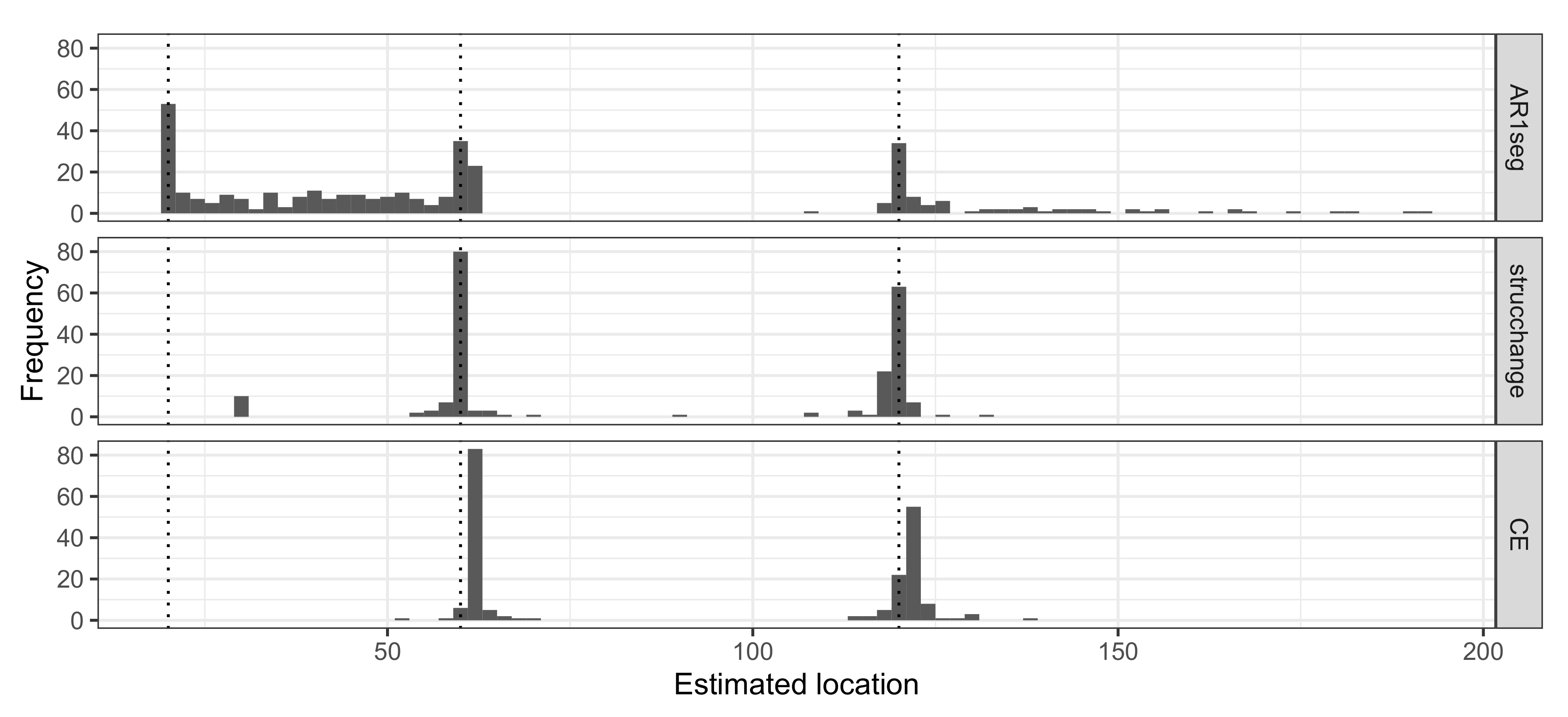
Figure 6 shows the frequency of estimated locations for each method under the Table 6 scenario with at least one change-point detected. The AR1seg method tends to estimate the first change-point location accurately. The CE.AR1 method has 100% power to identify the second and third locations; strucchange is less capable of detecting the first change-point at , while it performs well at and . It is noted that all the estimations obtained from CE.AR method cluster around 60 and 120 and tend to ignore the earliest location.
5. Discussion
In this section, we aim to recapitulate the discussion of the results of the numerical experiments. We will also apply the proposed method to real data analysis.
5.1. Simulation Results
The objective of the simulation study was to evaluate the performance of the three change-point detection methods (AR1seg and strucchange and the proposed CE.AR) under various scenarios looking at two aspects of the methods’ detection accuracies: the number of estimated change-points and their locations. We use tables to summarize the estimated number of change-points, while histograms are used to measure the detection accuracy in change-point locations. The simulation study consists of three examples. In the first example, there is no change-point in the AR(1) process; the CE.AR method achieves 100% exact detection rate under each of the three choices of the autocorrelation coefficient, 0.1, 0.5, and 0.9. The second example includes two scenarios, in which we study how a change in either the mean or the autocorrelation coefficient affects the performances of the algorithms. In scenario 1, it can be seen that the detection accuracy of the CE.AR method significantly improves as the shift in the mean increases from 1 to 3. In scenario 2, the autocorrelation coefficients differ between adjacent segments; we have considered six cases, whose profiles are shown in Figure 5. The cases with weak changes in the autocorrelation coefficient, such as , ; , ; or , , remain a challenge for the CE.AR method; it showed a heavy under-segmentation. In the third example, we consider a combined effect of the mean shift and the autocorrelation coefficient variation on piecewise AR(1) with multiple change-points. The two scenarios in this example show that the CE.AR method tends to disregard the first small segment, even if the mean or the autocorrelation coefficient changes dramatically. The histograms and Hausdorff distance show a low variation in estimated locations of change-points for the CE.AR method.
5.2. Application
We use a new real data set to demonstrate the practical aspects of our algorithm. The data were downloaded from the Reserve Bank of Australia—the daily AUD/CNY exchange rate from 2nd January 2018 to 24th March 2020. Both ARIMA and AR models have been used in the literature to model different exchange rates [48,49,50]. If an ARIMA process is used to model an exchange rate, then a change-point is recorded as a change in either the coefficients of AR part, or the MA part, or both of them. Dealing with the parameter change in the MA part of ARIMA process will be a matter of our future research. Before applying the CE.AR method, the stationary test and pre-examination are needed; the first difference of AUD/CNY is non-stationary, and we can get the rough profile of this series by using auto.arima() function which is built in forecast package [51]. If there is no obvious change in autocorrelation coefficient but in the mean level, AR1seg or the similar methods are preferred.
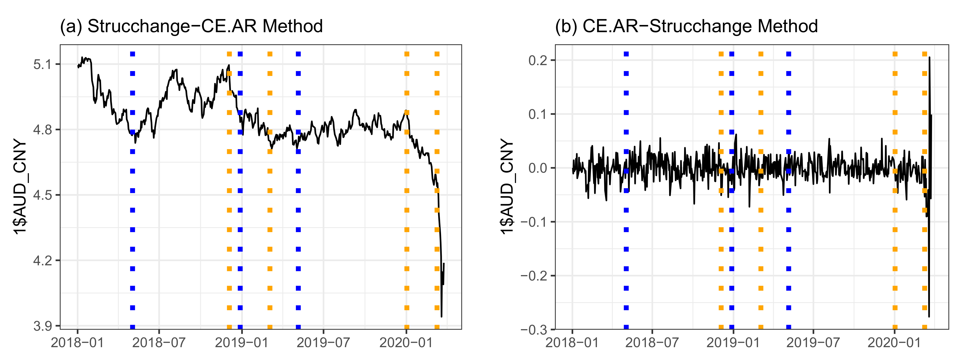
Figure 7 shows the estimation results obtained by the CE.AR and strucchange method. Since the actual number and the locations of change-points can not be identified in advance, we need to take both methods into account and seek for the agreement between them. The CE.AR method yields four possible change-points in 4 December 2018, 4 March 2019, 2 January 2020, and 9 September 2020, while strucchange” method presents three change-points that occurred in 3 May 2018, 28 February 2018, and 6 May 2019. Both methods have correctly identified the period from December of 2018 to May of 2019, and it seems that a regime started around 4 March 2019. According to the CE.AR method, the new regime started on 9 March 2020, so it managed to identify a very volatile period related to the COVID-19 pandemic.
If we bring the views from data itself to the real world, the cause of the changes may be the fallout from the China–United States trade war since 2018 or the uncertain climate in the Eurozone. The external shock has an impact on the Australian market, which has been reflected by the data and the estimated change points.
Hence, we suggest that the CE.AR algorithm would be a good tool for analyzing the daily AUD/CNY exchange rate; combined with the strucchange method, it will reveal more historical information. Forecasting the exchange rate based on the recent change-points will be done in the future research.
6. Conclusions
In this paper, we have proposed a new change-point detection algorithm, named CE.AR. The algorithm is able to detect change-points in piecewise AR(p) sequences, allowing variations in all parameters of the model. Our method involves two steps. Firstly, we build the MDL-based objective function to estimate the correct number of AR(p) segments. Then, we apply the Cross-Entropy algorithm for solving the combinatorial optimization problem. The numerical results show that, when the mean and the autoregression coefficient change moderately or strongly, the CE.AR method is very efficient at estimating multiple change-points. The Cross-Entropy algorithm also shows superior performance in detecting the locations of change-points. These two features make the proposed algorithm very useful from a practical point of view. We have demonstrated its usefulness by applying it to the latest real data set on the AUD/CNY exchange rate. The model considered here assumes an AR process; generalization to an ARIMA model is a matter for our further research. A limitation of the method comes from the under-segmentation when there is a small change in the mean or the autocorrelation coefficient. The improvement of detection accuracy for this problem needs to be taken into consideration in future research. In addition, it may be worth examining the impact of the lengths of the segments on the performance of the algorithm. Lastly, the question of whether our method would be helpful to improve the forecast’s accuracy is also a topic for our future research.
Author Contributions
Methodology, G.S.; software, L.M.; validation, L.M.; formal analysis, L.M.; investigation, L.M.; resources, G.S.; data curation, L.M.; writing—original draft preparation, L.M. and G.S.; writing—review and editing, G.S.; visualization, L.M.; supervision, G.S.; project administration, G.S.;funding acquisition, G.S. All authors have read and agreed to the published version of the manuscript.
Funding
This research received no external funding.
Acknowledgments
The authors would like to thank Dr Justin Whishart for reviewing the original manuscript and providing useful suggestions on programming.
Conflicts of Interest
The authors declare no conflict of interest.
Abbreviations
The following abbreviations are used in this manuscript:
| AR | Autoregressive |
| AR(1) | Autoregressive model of order 1 |
| AR(p) | Autoregressive model of order p |
| MDL | Minimum description length |
| AIC | Akaike’s information criterion |
| BIC | Bayesian information criterion |
| mBIC | Modified Bayesian information criterion |
| ShrinkageIC | A penalty function with an adjustable shrinkage parameter |
| CL | Code length |
| EM | Expectation-maximization |
| MCMC | Markov chain Monte Carlo |
| CE | Cross-Entropy |
| ARIMA | Autoregressive integrated moving average |
| MA | Moving average |
| AUD | Australian dollar |
| CNY | Chinese yuan |
References
- Aminikhanghahi, S.; Cook, D.J. A survey of methods for time series change point detection. Knowl. Inf. Syst. 2017, 51, 339–367. [Google Scholar] [CrossRef] [PubMed] [Green Version]
- Aue, A.; Horváth, L. Structural breaks in time series. J. Time Ser. Anal. 2013, 34, 1–16. [Google Scholar] [CrossRef]
- Zhu, X.; Li, Y.; Liang, C.; Chen, J.; Wu, D. Copula based Change Point Detection for Financial Contagion in Chinese Banking. Procedia Comput. Sci. 2013, 17, 619–626. [Google Scholar] [CrossRef] [Green Version]
- Bai, J.; Perron, P. Computation and analysis of multiple structural change models. J. Appl. Econom. 2003, 18, 1–22. [Google Scholar] [CrossRef] [Green Version]
- Garcia, R.; Perron, P. An Analysis of the Real Interest Rate Under Regime Shifts. Rev. Econ. Stat. 1996, 78, 111–125. [Google Scholar] [CrossRef] [Green Version]
- Beaulieu, C.; Chen, J.; Sarmiento, J.L. Change-point analysis as a tool to detect abrupt climate variations. Philos. Trans. R. Soc. 2012, 370, 1228–1249. [Google Scholar] [CrossRef] [Green Version]
- Davis, R.A.; Lee, T.C.M.; Rodriguez-Yam, G.A. Structural break estimation for nonstationary time series models. J. Am. Stat. Assoc. 2006, 101, 223–239. [Google Scholar] [CrossRef]
- Priyadarshana, W.; Sofronov, G. Multiple break-points detection in array CGH data via the cross-entropy method. IEEE/ACM Trans. Comput. Biol. Bioinform. (TCBB) 2015, 12, 487–498. [Google Scholar] [CrossRef]
- Sofronov, G.; Polushina, T.; Priyadarshana, M. Sequential Change-Point Detection via the Cross-Entropy Method. In Proceedings of the 11th Symposium on Neural Network Applications in Electrical Engineering (NEUREL2012), Belgrade, Serbia, 22 September 2012; pp. 185–188. [Google Scholar]
- Brodsky, B.; Darkhovsky, B.S. Non-Parametric Statistical Diagnosis: Problems and Methods; Springer Science & Business Media: Dordrecht, The Netherlands, 2000; Volume 509. [Google Scholar]
- Fryzlewicz, P. Wild binary segmentation for multiple change-point detection. Ann. Stat. 2014, 42, 2243–2281. [Google Scholar] [CrossRef]
- Raveendran, N.; Sofronov, G. Binary segmentation methods for identifying boundaries of spatial domains. In Communication Papers of the 2017 Federated Conference on Computer Science and Information Systems (FedCSIS); Ganzha, M., Maciaszek, L., Eds.; Polskie Towarzystwo Informatyczne: Warszawa, Poland, 2017; Volume 13, pp. 95–102. [Google Scholar] [CrossRef] [Green Version]
- Scott, A.J.; Knott, M. A cluster analysis method for grouping means in the analysis of variance. Biometrics 1974, 30, 507–512. [Google Scholar] [CrossRef] [Green Version]
- Sen, A.; Srivastava, M.S. On tests for detecting change in mean. Ann. Stat. 1975, 3, 98–108. [Google Scholar] [CrossRef]
- Auger, I.E.; Lawrence, C.E. Algorithms for the optimal identification of segment neighborhoods. Bull. Math. Biol. 1989, 51, 39–54. [Google Scholar] [CrossRef]
- Bai, J.; Perron, P. Estimating and testing linear models with multiple structural changes. Econometrica 1998, 66, 47–78. [Google Scholar] [CrossRef]
- Killick, R.; Fearnhead, P.; Eckley, I.A. Optimal detection of changepoints with a linear computational cost. J. Am. Stat. Assoc. 2012, 107, 1590–1598. [Google Scholar] [CrossRef]
- Bansal, N.K.; Du, H.; Hamedani, G. An application of EM algorithm to a change-point problem. Commun. Stat. Theory Methods 2008, 37, 2010–2021. [Google Scholar] [CrossRef]
- Doerr, B.; Fischer, P.; Hilbert, A.; Witt, C. Detecting structural breaks in time series via genetic algorithms. Soft Comput. 2016, 1–14. [Google Scholar] [CrossRef]
- Polushina, T.; Sofronov, G. Change-point detection in biological sequences via genetic algorithm. In Proceedings of the IEEE Congress on Evolutionary Computation (CEC’2011), New Orleans, LA, USA, 8 June 2011; pp. 1966–1971. [Google Scholar]
- Raveendran, N.; Sofronov, G. Identifying Clusters in Spatial Data via Sequential Importance Sampling. In Recent Advances in Computational Optimization: Results of the Workshop on Computational Optimization WCO 2017; Fidanova, S., Ed.; Springer International Publishing: Cham, Switzerland, 2019; pp. 175–189. [Google Scholar] [CrossRef]
- Sofronov, G.Y.; Evans, E.G.; Keith, J.M.; Kroese, D.P. Identifying change-points in biological sequences via sequential importance sampling. Environ. Model. Assess. 2009, 14, 577–584. [Google Scholar] [CrossRef]
- Algama, M.; Keith, J. Investigating genomic structure using changept: A Bayesian segmentation model. Comput. Struct. Biotechnol. J. 2014, 10, 107–115. [Google Scholar] [CrossRef] [Green Version]
- Keith, J.M. Segmenting Eukaryotic Genomes with the Generalized Gibbs Sampler. J. Comp. Biol. 2006, 13, 1369–1383. [Google Scholar] [CrossRef]
- Sofronov, G. Change-Point Modelling in Biological Sequences via the Bayesian Adaptive Independent Sampler. Int. Proc. Comput. Sci. Inf. Technol. 2011, 5, 122–126. [Google Scholar]
- Polushina, T.V.; Sofronov, G.Y. A hybrid genetic algorithm for change-point detection in binary biomolecular sequences. In Proceedings of the IASTED International Conference on Artificial Intelligence and Applications (AIA 2013), Innsbruck, Austria, 11 February 2013; pp. 1–8. [Google Scholar]
- Priyadarshana, M.; Polushina, T.; Sofronov, G. A Hybrid Algorithm for Multiple Change-Point Detection in Continuous Measurements. In Proceedings of the International Symposium on Computational Models for Life Sciences, AIP Conference Proceedings, Sydney, Australia, 27–29 November 2013; Volume 1559, pp. 108–117. [Google Scholar] [CrossRef]
- Priyadarshana, M.; Polushina, T.; Sofronov, G. Hybrid algorithms for multiple change-point detection in biological sequences. Adv. Exp. Med. Biol. 2015, 823, 41–61. [Google Scholar] [CrossRef]
- Sofronov, G.; Polushina, T.; Jayawardana, M. An improved hybrid algorithm for multiple change-point detection in array CGH data. In Proceedings of the 22nd International Congress on Modelling and Simulation, Tasmania, Australia, 8 December 2017; pp. 508–514. [Google Scholar]
- Evans, G.E.; Sofronov, G.Y.; Keith, J.M.; Kroese, D.P. Estimating change-points in biological sequences via the Cross-Entropy method. Ann. Oper. Res. 2011, 189, 155–165. [Google Scholar] [CrossRef] [Green Version]
- Polushina, T.; Sofronov, G. Change-point detection in binary Markov DNA sequences by the Cross-Entropy method. In Proceedings of the 2014 Federated Conference on Computer Science and Information Systems, FedCSIS 2014, Warsaw, Poland, 10 September 2014; pp. 471–478. [Google Scholar] [CrossRef] [Green Version]
- Polushina, T.; Sofronov, G. A Cross-Entropy method for change-point detection in four-letter DNA sequences. In Proceedings of the 2016 IEEE Conference on Computational Intelligence in Bioinformatics and Computational Biology (CIBCB), Chiang Mai, Thailand, 7 October 2016; pp. 1–6. [Google Scholar]
- Priyadarshana, M.; Sofronov, G. A modified Cross-Entropy method for detecting change-points in the Sri-Lankan stock market. In Proceedings of the IASTED International Conference on Engineering and Applied Science, EAS 2012, Colombo, Sri Lanka, 27 December 2012; pp. 319–326. [Google Scholar] [CrossRef]
- Priyadarshana, M.; Sofronov, G. A modified Cross-Entropy method for detecting multiple change points in DNA count data. In Proceedings of the 2012 IEEE Congress on Evolutionary Computation, CEC 2012, Brisbane, Australia, 15 June 2012; pp. 1020–1027. [Google Scholar] [CrossRef] [Green Version]
- Sofronov, G.; Ma, L. Change-point detection in time series data via the Cross-Entropy method. In Proceedings of the 22nd International Congress on Modelling and Simulation, Tasmania, Australia, 8 December 2017; pp. 195–201. [Google Scholar]
- Yau, C.Y.; Zhao, Z. Inference for multiple change points in time series via likelihood ratio scan statistics. J. R. Stat. Soc. Ser. B 2016, 78, 895–916. [Google Scholar] [CrossRef]
- Chakar, S.; Lebarbier, E.; Lévy-Leduc, C.; Robin, S. A robust approach for estimating change-points in the mean of an AR(1) process. Bernoulli 2017, 23, 1408–1447. [Google Scholar] [CrossRef]
- Killick, R.; Eckley, I. Changepoint: An R Package for Changepoint Analysis. J. Stat. Softw. 2014, 58, 1–19. [Google Scholar] [CrossRef] [Green Version]
- Zhang, N.R.; Siegmund, D.O. A modified Bayes information criterion with applications to the analysis of comparative genomic hybridization data. Biometrics 2007, 63, 22–32. [Google Scholar] [CrossRef] [PubMed]
- Lavielle, M. Using penalized contrasts for the change-point problem. Signal Process. 2005, 85, 1501–1510. [Google Scholar] [CrossRef] [Green Version]
- Rissanen, J. Stochastic Complexity in Statistical Inquiry; World Scientific: Singapore, 1989. [Google Scholar]
- McLeod, A.; Zhang, Y.; Xu, C.; McLeod, M.A. Package ‘FitAR’; University Western Ontario: London, ON, Canada, 2013. [Google Scholar]
- Botev, Z.I.; Kroese, D.P.; Rubinstein, R.Y.; L’Ecuyer, P. Chapter 3—The Cross-Entropy Method for Optimization. In Handbook of Statistics; Rao, C., Govindaraju, V., Eds.; Elsevier: Amsterdam, The Netherlands, 2013; Volume 31, pp. 35–59. [Google Scholar] [CrossRef] [Green Version]
- Rubinstein, R.Y. Combinatorial optimization, cross-entropy, ants and rare events. In Stochastic Optimization: Algorithms and Applications; Springer: Boston, MA, USA, 2001; pp. 303–363. [Google Scholar]
- Rubinstein, R. The cross-entropy method for combinatorial and continuous optimization. Methodol. Comput. Appl. Probab. 1999, 1, 127–190. [Google Scholar] [CrossRef]
- Rubinstein, R.Y.; Kroese, D.P. The Cross-Entropy Method: A Unified Approach to Combinatorial Optimization, Monte-Carlo Simulation and Machine Learning; Springer: New York, NY, USA, 2004. [Google Scholar]
- Zeileis, A.; Leisch, F.; Hornik, K.; Kleiber, C. strucchange: An R Package for Testing for Structural Change in Linear Regression Models. J. Stat. Softw. 2002, 7, 1–38. [Google Scholar] [CrossRef] [Green Version]
- Alam, M.Z. Forecasting the BDT/USD exchange rate using autoregressive model. Glob. J. Manag. Bus. Res. 2012, 12, 85–96. [Google Scholar]
- Babu, A.; Reddy, S. Exchange rate forecasting using ARIMA, Neural Network and Fuzzy Neuron. J. Stock Forex Trad. 2015, 4, 1–5. [Google Scholar]
- Yıldıran, C.U.; Fettahoğlu, A. Forecasting USDTRY rate by ARIMA method. Cogent Econ. Financ. 2017, 5, 1335968. [Google Scholar] [CrossRef]
- Hyndman, R.; Khandakar, Y. Automatic time series forecasting: The forecast package for R. J. Stat. Softw. 2008, 27, 1–22. [Google Scholar] [CrossRef] [Green Version]
Figure 1.
Popular methods for model selection used in change-point problems.

Figure 2.
(a) The three samples of the simulated AR(1) process whose mean varies from to . (b) The sample with a shift from to . (c) The simulated sample from to .
Figure 2.
(a) The three samples of the simulated AR(1) process whose mean varies from to . (b) The sample with a shift from to . (c) The simulated sample from to .

Figure 3.
Frequency of the estimated locations filtered by the correct number of change-points; the true number was 100. (a) The results from mean shifts . (b) The results from mean shifts . (c)The results from .
Figure 3.
Frequency of the estimated locations filtered by the correct number of change-points; the true number was 100. (a) The results from mean shifts . (b) The results from mean shifts . (c)The results from .

Figure 4.
Under scenario 2, frequency of the estimated locations was filtered by the correct number of change-points; the true change-point number was 100. (a) The results under , . (b) The results under , . (c) The results under , .
Figure 4.
Under scenario 2, frequency of the estimated locations was filtered by the correct number of change-points; the true change-point number was 100. (a) The results under , . (b) The results under , . (c) The results under , .

Figure 5.
The figure describes the setting of scenario 2 in Example 2.2 by using one simulated AR(1) process. The plots display the autocorrelation coefficient variation: (a) from 0.1 to 0.5, (b) from 0.1 to 0.9, (c) from 0.5 to 0.9, (d) from −0.5 to 0.1, (e) from −0.5 to 0.5, and (f) from −0.5 to 0.9.

Figure 6.
Frequency of the estimated locations when ; the true profile of change-points is at 20, 60, 120.
Figure 6.
Frequency of the estimated locations when ; the true profile of change-points is at 20, 60, 120.

Figure 7.
The orange dotted line in the plot represents estimated change-points using CE.AR, while the blue line represents the change-points detected by the strucchange method. In (a), we show the comparison of two methods on the daily exchange rate of AUD/CNY. (b) The change-point detection resulted by applying both methods on the first difference of AUD/CNY daily exchange rate. The data were downloaded from https://www.rba.gov.au/statistics/historical-data.html.


Table 1.
The estimated number of change-points in an AR(1) with no change points.
| AR parameter | |||||||||
| Algorithm | 1 | 1 | 1 | ||||||
| AR1seg | 95% | 4% | 1% | 89% | 3% | 8% | 36% | 17% | 47% |
| strucchange | 97% | 3% | 0% | 100% | 0% | 0% | 94% | 5% | 1% |
| CE.AR | 100% | 0% | 0% | 100% | 0% | 0% | 100% | 0% | 0% |
Table 2.
The estimated number of change-points under scenario 1.
| Mean Shift | |||||||||
| Algorithm | |||||||||
| AR1seg | 58% | 29% | 13% | 20% | 65% | 15% | 10% | 68% | 22% |
| strucchange | 60% | 40% | 0% | 2% | 97% | 1% | 0% | 97% | 3% |
| CE.AR | 97% | 3% | 0% | 41% | 58% | 1% | 2% | 97% | 1% |
Table 3.
The estimated number of change-points under scenario 2.
| Coefficient Shift | , | , | , | ||||||
| Algorithm | |||||||||
| AR1seg | 82% | 6% | 12% | 29% | 9% | 62% | 46% | 10% | 44% |
| strucchange | 68% | 32% | 0% | 0% | 97% | 3% | 36% | 61% | 3% |
| CE.AR | 96% | 4% | 0% | 6% | 92% | 2% | 90% | 8% | 2% |
Table 4.
The estimated number of change-points under scenario 2.
| Coefficient Shift | , | , | , | ||||||
| Algorithm | |||||||||
| AR1seg | 2% | 0% | 98% | 47% | 9% | 44% | 84% | 5% | 11% |
| strucchange | 0% | 97% | 3% | 0% | 98% | 2% | 25% | 74% | 1% |
| CE.AR | 0% | 99% | 1% | 3% | 95% | 2% | 87% | 13% | 0% |
Table 5.
Estimated number of multiple change points.
| Algorithm | ||||||
|---|---|---|---|---|---|---|
| 0 | 1 | 2 | 4 | |||
| AR1seg | 26% | 8% | 25% | 10% | 31% | 0% |
| strucchange | 22% | 68% | 9% | 1% | 0% | 0% |
| CE.AR | 74% | 13% | 10% | 3% | 0% | 0% |
Table 6.
Estimated number of multiple change points.
| Algorithm | ||||||
|---|---|---|---|---|---|---|
| 0 | 1 | 2 | 4 | |||
| AR1seg | 3% | 1% | 10% | 23% | 63% | 0% |
| strucchange | 0% | 0% | 90% | 9% | 1% | 0% |
| CE.AR | 0% | 0% | 100% | 0% | 0% | 0% |
Table 7.
Hausdorff distance for each algorithm and two choices of the parameters.
| AR1seg | strucchange | CE.AR |
|---|---|---|
| 73 | 46 | 39 |
| 73 | 30 | 19 |
© 2020 by the authors. Licensee MDPI, Basel, Switzerland. This article is an open access article distributed under the terms and conditions of the Creative Commons Attribution (CC BY) license (http://creativecommons.org/licenses/by/4.0/).
Share and Cite
MDPI and ACS Style
Ma, L.; Sofronov, G. Change-Point Detection in Autoregressive Processes via the Cross-Entropy Method. Algorithms 2020, 13, 128. https://0-doi-org.brum.beds.ac.uk/10.3390/a13050128
AMA Style
Ma L, Sofronov G. Change-Point Detection in Autoregressive Processes via the Cross-Entropy Method. Algorithms. 2020; 13(5):128. https://0-doi-org.brum.beds.ac.uk/10.3390/a13050128
Chicago/Turabian StyleMa, Lijing, and Georgy Sofronov. 2020. "Change-Point Detection in Autoregressive Processes via the Cross-Entropy Method" Algorithms 13, no. 5: 128. https://0-doi-org.brum.beds.ac.uk/10.3390/a13050128
Note that from the first issue of 2016, this journal uses article numbers instead of page numbers. See further details here.