Sparse Logistic Regression: Comparison of Regularization and Bayesian Implementations

Abstract

In knowledge-based systems, besides obtaining good output prediction accuracy, it is crucial to understand the subset of input variables that have most influence on the output, with the goal of gaining deeper insight into the underlying process. These requirements call for logistic model estimation techniques that provide a sparse solution, i.e., where coefficients associated with non-important variables are set to zero. In this work we compare the performance of two methods: the first one is based on the well known Least Absolute Shrinkage and Selection Operator (LASSO) which involves regularization with an ${\ell }_1$ norm; the second one is the Relevance Vector Machine (RVM) which is based on a Bayesian implementation of the linear logistic model. The two methods are extensively compared in this paper, on real and simulated datasets. Results show that, in general, the two approaches are comparable in terms of prediction performance. RVM outperforms the LASSO both in term of structure recovery (estimation of the correct non-zero model coefficients) and prediction accuracy when the dimensionality of the data tends to increase. However, LASSO shows comparable performance to RVM when the dimensionality of the data is much higher than number of samples that is $p>>n$.

1. Introduction

Techniques for the estimation of sparse models have gained increasing attention in the last two decades and have found several practical applications in different areas of science and engineering. Example applications include biomedical [1], home automation [2], manufacturing [3,4], telecommunication [5] and social media analysis [6,7]. Often, in high dimensional settings, there is a high number of measured variables and not all of them are relevant in terms of correlation with the output. In these cases, sparse models are important to avoid overfitting and improve model prediction performance as well as to identify a subset of input variables representing the most important drivers of the output variation [8]. In this work, we discuss the variable selection capability of some sparse techniques and to this end, we recall that for variable selection there are three main families of techniques [8,9,10], according to the mechanism they use to perform the variable selection tasks: filter methods, wrapper methods and embedded methods.

Filter methods first identify a subset of variables, for example using correlation analysis, which is then used as input with standard algorithms. Wrapper methods embed the model search procedure within the variable subset search. A typical example of a wrapper method is the stepwise selection strategy [11]. Finally, embedded and wrapper methods estimate at the same time the model and select the most useful variables.

This work focuses on embedded methods and in particular, the most popular embedded method—the Least Absolute Shrinkage and Selection Operator. This method, better known as the LASSO [12] in the statistical community, or as “basis pursuit” in the signal processing community [13], is based on regularization with a ${\ell }_1$ norm which is known to induce sparseness in model coefficients. Other methods recently proposed are the Elastic-Net [14], which overcomes some drawbacks of the LASSO by incorporating a combination of ${\ell }_1$ and ${\ell }_2$ norms and the Relevance Vector Machine (RVM) [15], that resorts to a Bayesian framework.

Here, we compare the LASSO and RVM implementations for the estimation of a linear logistic regression model for classification tasks. The prediction accuracy and model recovery performance of each approach is investigated for both simulated and real benchmark datasets. Comparisons are performed within a Monte Carlo Cross-Validation framework to increase the robustness of the analysis. Many advanced solvers are available in the literature for ${\ell }_1$ logistic regression problem; for example, refs. [16,17] provide efficient procedures to solve related optimization tasks. There are several works dealing with the comparison of different algorithms for estimation of models with ${\ell }_1$ norm regularization, see for example [18,19], however, to the best of our knowledge, very few works in the literature provide a broad comparison on several datasets with different characteristics between LASSO and the RVM (see Section 2 for details on related work on the comparison between LASSO and RVM as well as other related methods for regularization). Moreover, an element of novelty provided by the present work, is the application of RVM and LASSO comparing them not only in terms of prediction accuracy but also in terms of structure recovery capacity on real industrial datasets, one related to a semiconductor manufacturing modeling problem referred to as Virtual Metrology and the other related to consumer goods soft sensing problem provided by Electrolux.

It seems to be important and useful to propose here a study based on different datasets discussing the main differences between these methods. As such, in this paper we provide a comparison between LASSO and RVM in terms of structure recovery and prediction accuracy on different datasets as a reference study for applications where model interpretability is a priority and interest is mainly focused on selecting the most powerful predictors for the response.

The present work is based on preliminary experimental comparisons reported in [20]; the goal of this extended version is to provide the readers with a well-rounded and detailed comparison between LASSO and RVM: w.r.t. [20] (i) we are providing here more detailed descriptions of the considered modeling approaches; (ii) we are covering additional real-world case studies and (iii) we are providing results not only in terms of accuracy, but also on structure recovery, i.e., the effectiveness of the methods in identifying the true informative predictors.

The outline of the paper is as follows: Section 2 summarizes literature on comparisons between the two techniques at hand. Section 3 briefly introduces the two techniques for estimating of the logistic model parameters, while Section 4 describes the Monte Carlo Cross-Validation framework employed to yield statistically robust comparisons. The performance metrics used to measure the performance of the two techniques are also introduced in Section 4.2. Section 5 introduces the benchmark datasets, and Section 6 presents and discusses the results. Finally, concluding remarks are given in Section 7.

2. Related Work

In this section, we review related works on comparisons between LASSO and RVM for sparse regression. The first of these [21] applies the Bayesian methodology to kernel regression (nonparametric regression) models and uses LASSO as an alternative approach (generalized LASSO) showing that this algorithm can be generalized to logistic regression which is being investigated here. Results demonstrate that the generalized LASSO model combines several advantages: on a conceptual level, it allows quantification of a confidence interval around the predicted values in a probabilistic way. It also describes RVM as similar to the generalized LASSO estimator since it shows a probabilistic interpretation of the fit to the data and the key concept of both is the use of automatic relevance determination (ARD) priors in a Bayesian viewpoint of regression. Some conclusions of [21] are:

• The LASSO combines the advantages of efficiently handling large training sets and producing extremely sparse solutions;
• The RVM has severe computational problems for large training sets;
• it is difficult to apply the RVM to large-scale real-world problems.

Basically, ref. [21] reformulates the relevance determination problem in the LASSO framework to use a highly efficient subset algorithm introduced in [22]. It represents one of the most important references for this paper but does not provide a comprehensive comparison between LASSO and RVM in terms of the diversity of datasets considered.

In [23], the authors show how the Bayesian variational algorithm is established for the kernelized LASSO introduced in [21] and investigate the method for learning kernel parameters under the kernelized LASSO formulation. The algorithm is called Bayesian Sparse Kernel Learning with LASSO (BSKL-LASSO) and has been proposed for solving kernel regression modeling problems with the LASSO penalty. The BSKL-LASSO method is tested on both a synthetic data set and one real-world data set. The experiments are used to assess the ability of BSKL-LASSO in learning kernel hyperparameters and also compare BSKL-LASSO to other related algorithms such as Tipping’s RVM [15]. The overall performance offered by the BSKL-LASSO algorithm is comparable to the performance of RVM in terms of finding sparse kernel models. Furthermore, in this case, the comparison between methods could be extended with a broader range of datasets.

Other references are available in the literature as examples of regression with binary output for real problems, for example, ref. [24] which addresses the problem of monitoring safety conditions in underground coal mines. In particular, this paper discusses practical methods for the assessment of seismic hazards using analytical models based on sensory data and domain knowledge to obtain an information system that can issue early warnings about seismic hazards in underground coal mines.

In [25], the authors present a statistical perspective on boosting [26] which can then be seen as an interesting regularization scheme for estimating a model; they also study the variable selection problem with boosting algorithms ([27,28]).

Another noteworthy contribution is the adaptive Lasso, introduced by Zou [29]. Consistency of the adaptive Lasso for variable selection has been proven for the high-dimensional case with $p>>n$ [30]. In [31], a unified account of boosting and logistic regression is given; both learning problems can be cast in terms of optimization of Bregman distances [32] and the result is an adaptation of boosting methods to the problem of minimizing the logistic loss used in logistic regression. In [33], the reader can find additional views on boosting; in particular, the relation between boosting and $l_1$-penalized estimation. This enabled new perspectives, namely to use boosting methods in many other contexts than classification.

It is also true that other several works on boosting methods for regression exist, for example, refs. [34,35]. In these proposals, boosting is not only a black-box prediction tool but also an estimation method for models with a specific structure such as linearity or additivity.

Boosting can then be seen as an interesting regularization scheme for estimating a model. In [36], authors focus on the classical linear discriminant analysis (LDA) or Fisher’s LDA [37]); here two simple sparse LDA variants that rely on a penalty function inspired by the RVM are introduced and is clear that the RVM is well-suited for integration with LDA. The aforementioned literature is suggested to the reader to provide some contexts for sparse regularized regression.

Sparse learners, such as the aforementioned LASSO and RVM, have gained popularity in process industry nowadays; it is the case of data driven Soft Sensors design ([38,39]). Soft Sensors (SS) are statistical model-based technologies used in industrial environments that provide an estimate of quantities that may be unmeasurable or costly/time-consuming to measure. In this scenario, a recent study on the most suitable learner for soft sensor design in process industries has been provided by [40] where authors assessed and compared predictive performances of three regression techniques: Partial Least Squares (PLS), LASSO and RVM using data from real industrial plants and a simulated process. That work highlighted a clear advantage in the use of sparse learners on large sets of predictors for the improvement of the prediction accuracy respect to PLS. Moreover, it shows occasional unstable predictions of RVM for small training sets recommending the use of RVM instead of LASSO only if a sufficiently large dataset is available for the design of a Soft Sensor.

The aim of this paper respect to [40], is to provide a tutorial reference for a broad comparison between LASSO and RVM not only in terms of prediction accuracy but also in terms of structure recovery capacity using several datasets (simulated and real) giving to the reader a broad-spectrum vision on the topic.

3. Methods

Formally, a linear logistic regression model is described in terms of the logistic linking function:

$${\sigma }_{\mathit{\theta }}\left(x_i\right)=\frac{1}{1+e^{-x_i\mathit{\theta }}}$$

(1)

where $\mathit{\theta }\in {\mathbb{R}}^p$ is a $(p\times 1)$ vector containing the coefficient of the linear model, $({\mathbf{x}}_{\mathbf{i}},y_i)$ are the input-output data points, where $x_i\in {\mathbb{R}}^p$ and $y_i\in \{0,1\}$ for $i=1,\dots ,n$ so that $\mathbf{y}={[y_1,\dots ,y_n]}^T$ is a $(n\times 1)$ vector and $\mathbf{X}={[x_1,\dots ,x_n]}^T$ a $(n\times p)$ matrix. Moreover, we consider the input $\mathbf{X}$ scaled to have zero mean such that we can consider the intercept term to be zero. We refer to linear logistic regression because there is a linear relationship between the data $x_i$ and the model coefficients $\mathit{\theta }$.

Estimation of the model coefficients $\mathit{\theta }$ in (1) is obtained by Maximum-Likelihood (ML). Assuming that the output variable y is distributed in logistic regression according to a Bernoulli distribution, the probability of the outcome for the i data point can be written in compact form as:

$$p\left(y_i\right|x_i;\mathit{\theta })={\sigma }_{\mathit{\theta }}{\left(x_i\right)}^{y_i}{(1-{\sigma }_{\mathit{\theta }}\left(x_i\right))}^{1-y_i}$$

(2)

The likelihood $L\left(\mathit{\theta }\right)$ of the model given the data is then obtained considering the contribution of all the n data points:

$$L\left(\mathit{\theta }\right)=p\left(\mathbf{Y}\right|\mathbf{X};\mathit{\theta })=\prod _{i=1}^{n}p\left(y_i\right|x_i;\mathit{\theta })=\prod _{i=1}^n{\sigma }_{\mathit{\theta }}{\left(x_i\right)}^{y_i}{(1-{\sigma }_{\mathit{\theta }}\left(x_i\right))}^{1-y_i}$$

(3)

The parameter vector $\mathit{\theta }$ is finally estimated by maximizing the logarithm of the likelihood (3):

$$l\left(\mathit{\theta }\right)=logL\left(\mathit{\theta }\right)=\sum _{i=1}^n{y}_{i}log\left({\sigma }_{\mathit{\theta }}\left(x_i\right)\right)+(1-y_i)log(1-{\sigma }_{\mathit{\theta }}\left(x_i\right))$$

(4)

In other words, the estimated model coefficients are those that maximize the probability (or likelihood) of having generated the data. The ML estimate is prone to overfitting [33], especially in high dimensional problems where there are many and possibly correlated input variables. For this reason, sparse classification techniques are useful because they select only a limited number of input variables which generally yields better generalization performance. In the next Sections, we briefly describe the LASSO and RVM implementations of the logistic model (1).

3.1. Least Absolute Shrinkage and Selection Operator (LASSO)

In the context of classification with a logistic regression model, the ${\ell }_1$ norm regularized logistic regression problem consists of estimating the model coefficients collected in $\mathit{\theta }$ by minimizing a cost function given by the sum of the log-likelihood (4) and a regularization term consisting of the sum of the absolute values of the model coefficients (i.e., the ${\ell }_1$ norm of the vector of coefficients):

$$l_R\left(\mathit{\theta }\right)=\sum _{i=1}^n\{y_{i}log\left({\sigma }_{\mathit{\theta }}\left(x_i\right)\right)+(1-y_i)log(1-{\sigma }_{\mathit{\theta }}\left(x_i\right))\}-\lambda \sum _{j=1}^p\left|{\mathit{\theta }}_j\right|$$

(5)

The trade-off between likelihood maximization and model complexity is governed by the regularization parameter $\lambda \in {\mathbb{R}}^{+}$ and is usually selected by cross-validation (see Section 4). First, note that a quadratic approximation to the unpenalized cost function (4) about the current estimate (Taylor expansion about current estimates) is given by (see [33,41] for details)

$${\ell }_Q\left(\mathit{\theta }\right)=-\frac{1}{2n}\sum _{i=1}^n{w}_i{(z_i-x_i\mathit{\theta })}^2$$

(6)

where

$$z_i=x_i\mathit{\theta }+\frac{y_i-{\sigma }_{\mathit{\theta }}\left(x_i\right)}{{\sigma }_{\mathit{\theta }}\left(x_i\right)(1-{\sigma }_{\mathit{\theta }}\left(x_i\right))}$$

(7)

and

$$w_i={\sigma }_{\mathit{\theta }}\left(x_i\right)(1-{\sigma }_{\mathit{\theta }}\left(x_i\right)).$$

(8)

The LASSO algorithm is a popular regularization method for model coefficient estimation and variable selection [12] which can be used to solve (5) with the same quadratic approximation for the unpenalized cost function ([41]), i.e., to solve:

$$\underset{\mathit{\theta }}{min}\{-{\ell }_Q\left(\mathit{\theta }\right)+\lambda \sum _{j=1}^p|{\theta }_j\left|\right\}$$

(9)

cycling through all variables $j=1,2,\dots ,p$ until a certain criterion is met. For each value of $\lambda$, an outer loop computes the quadratic approximation about the current parameters $\mathit{\theta }$, then the coordinate descent path algorithm ([33,42]) solves the penalized weighted least-squares problem (9).

3.2. Relevance Vector Machine (RVM)

Here, the linear logistic model, whose likelihood is described by (3), is formulated within a Bayesian framework where sparseness is encoded by setting priors on the model coefficients ${\theta }_j$. This a priori information, i.e., the knowledge, before looking at the data, that all variables are important, is updated during the learning process where evidence from the data is used to set ${\theta }_j$ corresponding to non-infomative variables to zero. This implementation, called the Relevance Vector Machine [15], estimates the posterior distribution of the parameter vector $\mathit{\theta }$ and the hyperparameters $\mathit{\alpha }\in {\mathbb{R}}^p$ governing sparseness (see below) over the data. Therefore, from Bayesian representation:

$$p(\mathit{\theta },\mathit{\alpha }|\mathbf{Y})=\frac{p\left(\mathbf{Y}\right|\mathit{\theta },\mathit{\alpha }\left)p\right(\mathit{\theta },\mathit{\alpha })}{p\left(\mathbf{Y}\right)}$$

(10)

where $p\left(\mathbf{Y}\right|\mathit{\theta },\mathit{\alpha })$ is the likelihood function and $p(\mathit{\theta },\mathit{\alpha })$ is the prior distribution defined over the model coefficients and the hyperparameters, respectively. The hyperparameter vector $\mathit{\alpha }$ is encoded as a zero-mean Gaussian distribution over $\mathit{\theta }$ (popular simple choice discussed in [15]):

$$p\left(\mathit{\theta }\right|\mathit{\alpha })=\prod _{j=1}^p\mathcal{N}\left({\theta }_j|0,{\alpha }_j^{-1}\right)$$

(11)

and a further set of hyperparameters Gamma distributed over the $\mathit{\alpha }$ vector is then introduced; for further details the interested reader is referred to [15]. Given a test data point $\tilde{x}$, predictions are made for the corresponding target $\tilde{y}$, in terms of the predictive distribution:

$$p\left(\tilde{y}\right|\mathbf{Y})=\int p\left(\tilde{y}\right|\mathit{\theta },\mathit{\alpha })p(\mathit{\theta },\mathit{\alpha }|\mathbf{Y})d\mathit{\theta }d\mathit{\alpha }$$

(12)

The posterior (10) cannot be computed because the normalizing integral on the right-hand-side $p\left(\mathbf{Y}\right)=\int p\left(\mathbf{Y}\right|\mathit{\theta },\mathit{\alpha }\left)p\right(\mathit{\theta },\mathit{\alpha })d\mathit{\theta }d\mathit{\alpha }$ cannot be obtained analytically. The posterior is thus decomposed as:

$$p(\mathit{\theta },\mathit{\alpha }|\mathbf{Y})=p(\mathit{\theta }|\mathit{\alpha },\mathbf{Y})p\left(\mathit{\alpha }\right|\mathbf{Y}).$$

(13)

An iterative algorithm can then be used, where an estimate of $\mathit{\alpha }$ given by the second term on the right-hand side of (13) is used to calculate $\mathit{\theta }$; this is then used to update the previous estimation of $\mathit{\alpha }$. In particular, the posterior of $\mathit{\theta }\sim \mathcal{N}\left({\mathit{\theta }}^{RVM},{\mathsf{\Sigma }}^{RVM}\right)$ in terms of the parameters of a Gaussian distribution $({\mathit{\theta }}^{RVM},{\mathsf{\Sigma }}^{\mathbf{RVM}})$ can be found by maximizing the first term on the right-hand-side of (13) [43]. The vector ${\mathit{\theta }}^{RVM}$ is obtained by maximizing the quantity $p\left(\mathit{\theta }\right|\mathit{\alpha },\mathbf{Y})\propto p(\mathbf{Y}\left|\mathit{\theta }\right)p\left(\mathit{\theta }\right|\mathit{\alpha })$ using a second order Newton gradient ascent method, once it is written in the following form discussed in [15]:

$$log\left(p\left(\mathbf{Y}\right|\mathit{\theta })p\left(\mathit{\theta }\right|\mathit{\alpha })\right)=l\left(\mathit{\theta }\right)-\frac{1}{2}\left\{{\mathit{\theta }}^T\mathit{A}\mathit{\theta }\right\}$$

(14)

where $\mathit{A}=diag({\alpha }_1,\dots ,{\alpha }_p)$. Note that (14) is a regularized version of the log-likelihood function (4) and that there is a hyperparameter ${\alpha }_j$ associated with each coefficient and thus each variable of the logistic model. A Laplace approximation is then used to calculate ${\mathsf{\Sigma }}^{RVM}$ [43]. Once an estimate of $\mathit{\theta }\sim \mathcal{N}\left({\mathit{\theta }}^{RVM},{\mathsf{\Sigma }}^{RVM}\right)$ is obtained, hyperparameter learning is performed by calculating the posterior for the second part of the right-hand-side of (13), i.e., the maximization of $p\left(\mathit{\alpha }\right|\mathbf{Y})\propto p(\mathbf{Y}\left|\mathit{\alpha }\right)p\left(\mathit{\alpha }\right)$ (the reader can find all steps described both in [44,45]). This gives

$${\alpha }_j^{new}=\frac{1-{\alpha }_j{\mathsf{\Sigma }}_{jj}^{RVM}}{{\left({\theta }_j^{RVM}\right)}^2}$$

(15)

The above formulation of the prior distributions is also known as automatic relevance determination (ARD) [46,47]. The entire algorithm used here is explained in [44] and the reader is also addressed to [45] for a comprehensive review of that work with implementation details reported.

The basic idea of ARD is that only important variables are selected if there is enough evidence in the data. The priors over the model coefficients are initialized with large values (small ${\alpha }_j$’s) in such a way that all the variables are considered important at the beginning. The evidence from the data will then concentrate the posterior probability at very large values for some of the ${\alpha }_j$, with the consequence that the posterior probability of the associated weight will be concentrated to zero, effectively “switching off” the corresponding variable.

As stated in [45], the RVM process is an iterative one and involves repeatedly re-estimating hyperparameters such as ${\alpha }_j$ in (15) until a stopping criterion is met. In particular, a threshold value ${\delta }_{Thresh}$ is chosen to obtain a stopping condition computing the change between one iteration’s estimation of ${\alpha }_j$ and the next: $\delta ={\sum }_{j=1}{\alpha }_j^{new}-{\alpha }_j$, so that re-estimation will stop when $\delta <{\delta }_{Thresh}$. Another threshold value established in the algorithm is ${\alpha }_{Thresh}$ which is assumed an ${\alpha }_j$ is tending to infinity upon reaching it. Additional details on values chosen for such thresholds will be provided in Section 4.3.

A practical advantage of this formulation is that the model complexity is automatically determined by the data through ARD and thus the RVM model does not need a cross-validation step to optimize model complexity.

The RVM originally was presented as a possible alternative to Support Vector Machines (SVM) because of its sparsity property [15]. When the so-called “kernel trick” is applied, the RVM is similar to SVM since it returns sparse models in the observation space, highlighting the “relevant” data points that are the equivalent of the “support” data point in the SVM model. In this work, RVM is applied to linear kernel models and we are interested in variable rather than data point selection, thus we consider the linear model (1) where the hyperpriors are defined over the input variable coefficients ${\theta }_j$.

4. Model Setting

Assessing the quality of a model on a set of observations of the phenomena that has not being used for model construction is essential for a fair evaluation of the prediction performance of the proposed model; for this reason, the available dataset of n samples is usually divided into two parts:

• a training dataset ($qn$ samples, where $0<q<1$), which is used to construct the model;
• a test dataset ($(1-q)n$ samples), which is used to assess the quality of the estimated model.

When only a limited number of observations is available, the quality of the model strongly depends on the split of the data. To avoid data related bias when evaluating the performance of models, Monte Carlo Cross-Validation (MCCV), can be used as described below.

4.1. Monte Carlo Cross-Validation

The Monte Carlo Cross-Validation (MCCV) procedure, which is also called repeated random sub-sampling validation [48] or repeated trining-test split or leave-group-out cross-validation in literature [49], as described in Algorithm 1 below, performs an analysis on $K_1$ different random splits of the available observations into training/test datasets. Thus, $K_1$ different models are built and the performance of the models is assessed as the average model performance over $K_1$ simulations. For consistent results, $K_1$ needs to be a large number (of the order of hundreds/thousands). The number of repetitions is important. Increasing the number of subsets has the effect of decreasing the uncertainty of the performance estimates. This is also a function of the proportion of samples were randomly allocated to the prediction set; the larger the percentage, the more repetitions are needed to reduce the uncertainty in the performance estimates [49].

Moreover, in a classification problem, the dataset can be unbalanced, with one class having a much lower number of instances than the other one. To handle this problem, an undersampling strategy can be used where at each Monte Carlo (MC) iteration a new dataset is built randomly undersampling the most numerous class. After balancing the dataset, the choice is to split it into training and test part; these parts may not be balanced, so another choice could be to insert a stratified procedure to guarantee proportions of the two classes are maintained [50].

A K-fold Cross-Validation (CV) procedure estimates the LASSO regularization parameter $\lambda$ at step 6 of Algorithm 1. This procedure involves splitting the training set into K approximately equal parts. Each part is then selected in turn as a validation dataset and the remaining $K-1$ parts used to estimate the model, which is evaluated on the validation dataset. The CV error is defined as the average of the misclassification error (MCE) (see Section 4.2) achieved on the K validation sets. The CV error is computed for a range of $\lambda$ values and the value that yields the minimum CV error is selected as the optimum.

Step 6 in Algorithm 1 is repeated $K_2$ times and the median among the $K_2$ complexity values is used to estimate the model during the i-th MC iteration. One difference between MCCV and k-fold cross-validation is that samples can be represented in multiple held-out subsets. Furthermore, the number of repetitions is usually larger than in k-fold cross-validation i.e., $K_1>K_2$; in this case a choice of $K_1=1000$ and $K_2=10$ was made.

Algorithm 1: Monte Carlo Cross-Validation algorithm.

4.2. Performance Metrics

Different kinds of metrics are considered for measuring the performance of the two techniques both in terms of structure discovery and output prediction accuracy. The effectiveness of discovering the true underlying model structure is measured in terms of True Positive (TP) and True Negative (TN) rates calculated with respect to the true $\mathit{\theta }$ (expressed in percentage). The estimated model vectors with RVM $\left({\mathit{\theta }}_{\mathit{RVM}}\right)$ and LASSO $\left({\mathit{\theta }}_{\mathit{LASSO}}\right)$ are compared with the true one as generated in Section 5.1 for each case. The True Positive Rate (TP) is defined as the fraction of ${\theta }_j$ different from zero estimated correctly out of the total number of coefficients p. On the other hand, the True Negative Rate (TN) is defined as the fraction of ${\theta }_j$ equal to zero estimated correctly.

Classification accuracy is measured in terms of Misclassification Error (MCE), comparing the true output y with the one estimated by the two models. At each MC iteration, the MCE is calculated on the test data set as the number of errors in predicting the outcome variables (e) normalized by the number of points in the test dataset ($(1-q)n$):

$${\mathrm{MCE}}_k=\frac{e}{(1-q)n}k=1,\cdots ,K_1$$

(16)

Model prediction accuracy is also measured using the Receiver Operating Characteristic (ROC) curves showing the True Positive Rate (fraction of true positives out of the total actual positives) also called sensitivity $vs.$ the False Positive Rate (fraction of false positives out of the total actual negatives) for various threshold values. Hereafter, specificity will be the reference for the true negative rate, i.e., the proportion of actual negatives that are correctly identified as such. The Area Under the Curve (AUC) can be calculated from the ROC curves, and is considered here to summarize the results obtained with Algorithm 1, since it would be infeasible to plot ROC curves for each $K_1$ MC simulation. The AUC $\in [0,1]$ where “1” indicates the “perfect” model, while “0.5” indicates a completely random guess.

4.3. Simulation Setup

Free available software implementations were used for Simulations (Matlab libraries: glmnet (http://www.stanford.edu/~hastie/glmnet_matlab/) for LASSO and Sparse Bayesian Modeling (http://www.miketipping.com/sparsebayes.htm) for RVM). In all simulations, the percentage of data used for training is $70\%$ with a cycle of $K_1=1000$ iterations for MCCV and an inner cycle of $K_2=10$ iterations for K-fold as explained in Section 4.1. As regards the choice for thresholds related to the RVM hyperparameters introduced before in Section 3.2, default numerical values available in the library have been taken into account and reported here:

• ${\alpha }_{Thresh}={10}^{-12}$: any “relevance factor” less than this threshold is considered to be zero;
• ${\delta }_{Thresh}={10}^{-3}$: if the change in the log-likelihood function (14) for the best re-estimation is less than this, we consider termination.

According to the RVM methodology explained before in Section 3.2, the chosen hyperparameters are the ones that maximize the log-likelihood from the initial values (following the default choice for the initialization in [44]) and using (15) to calculate new estimates and repeating the process until convergence is met with the abovementioned thresholds.

5. Datasets

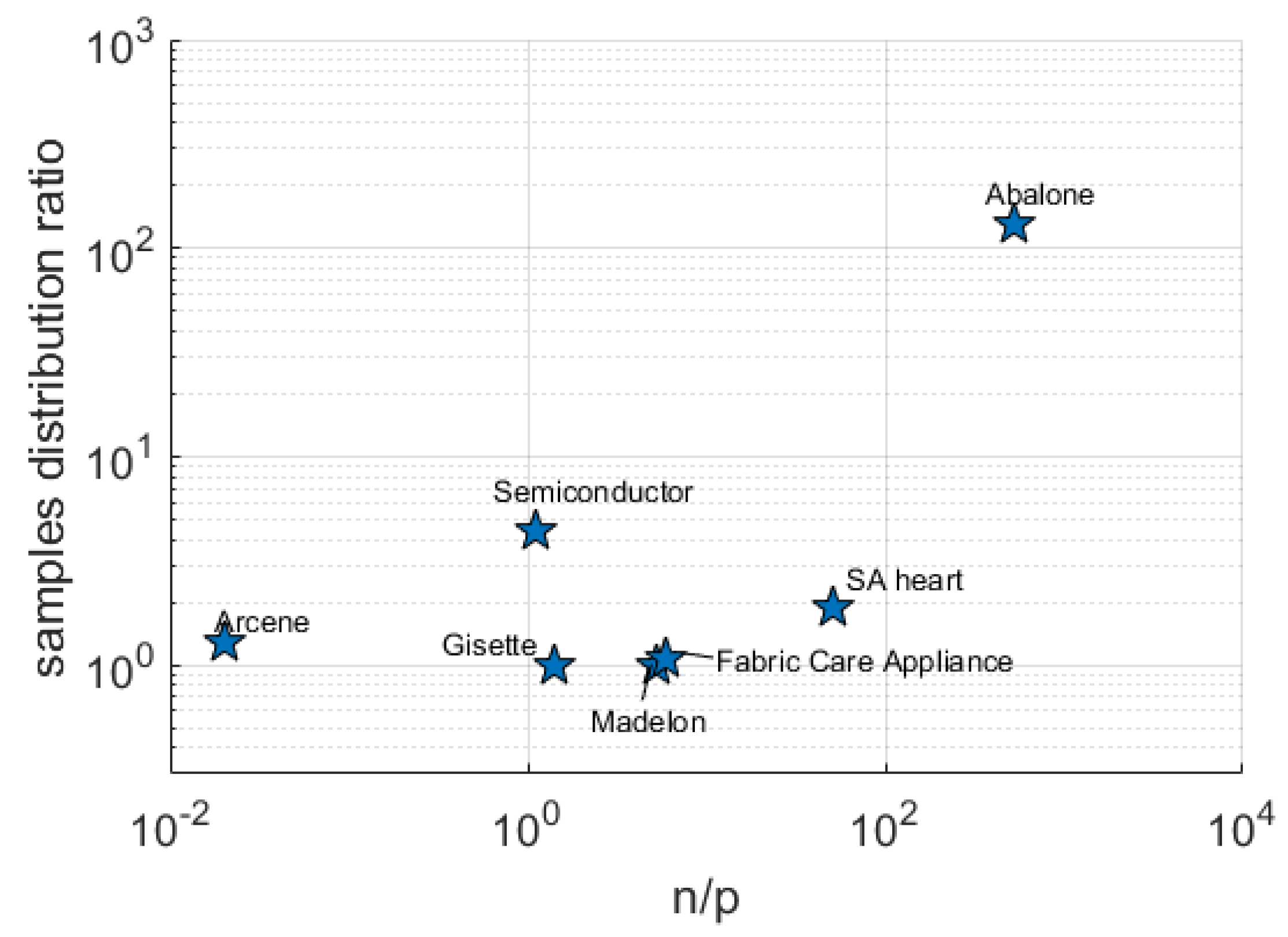
To test the abilities of RVM and LASSO with respect to discovering the true model structure and predicting the correct class, we consider both real and simulated data sets. These datasets consist of binary output values, i.e., $y=\{0,1\}$, present different characteristics in terms of p and n values and have different ratios between the number of samples belonging to the different classes. A summary of these characteristics for the real datasets are presented in

Table 1. Real datasets summary. The last column indicates the number of observations belonging to each of two classes. Madelon is an artificial dataset and included here among real data.

	Observations	Variables	Samples Distribution
	(n)	(p)	($\mathit{k}=0,1$) [Ratio]
SA heart	462	9	160/302
Abalone	4174	8	32/4132
Semiconductor	2194	1988	410/1784
Arcene	200	10,000	88/112
Madelon	2600	500	1300/1300
Gisette	7000	5000	3500/3500
Fabric Care Appliance	304	52	146/158

and Figure 1 while the simulated datasets are described in the following subsection.

5.1. Simulated/Artificial Data

The simulated datasets are generated by imposing a certain correlation structure on the input matrix $\mathbf{X}$:

(a)

Independent predictor variables: all $p=100$ predictor variables are IID standard normal distributed; sample size $n=100$ and $n=1000$;

(b)

Toeplitz design: the $p=100$-dimensional predictor variables follow an $\mathcal{N}(0,\mathsf{\Sigma })$ distribution, where $\mathsf{\Sigma }={\rho }^{|k-m|}$ and $\rho =0.99$; sample size $n=200$ and $n=1000$; $k,m=1,\dots ,p$. Therefore $\mathsf{\Sigma }$ is a matrix of p rows and p columns made up by all combinations of $\rho$, k, m.;

(c)

Factor model with two factors: let ${\varphi }_1$ and ${\varphi }_2$ be two latent variables following IID standard normal distributions. Each predictor variable $x_k$, for $k=1,\dots ,p$, is generated as a combination of gaussians $x_k=f_{k,1}{\varphi }_1+f_{k,2}{\varphi }_2+{\eta }_k$, where $f_{k,1},f_{k,2}$ and ${\eta }_k$ have IID standard normal distributions for all $k=1,\dots ,p$; sample sizes are $n=200$ and $n=1000$ while $p=100$;

(d)

Data set (d) is identical to (c) but with 10 instead of two factors;

(e)

All simulations (a)–(d) are repeated with $p=1000$.

(f)

Manufacturing dataset: as shown in Figure 2, this dataset shows high block-correlation among subsets of input variables and has $p=1988$ and $n=2194$ (the Pearson correlation coefficient was used for the computation [51]). The variables represent statistical moments (Mean, Variance, Skewness and Kurtosis), calculated from Optical Emission Spectroscopy (OES) data from a plasma etching process. Independent variables of this dataset are used in this paper to obtain a first case study for simulated/artificial environment (constructing a simulated output) in order to study prediction accuracy and model recovery for different $(n,p)$. In this case we know which variables are truly relevant. A second case study for real environment (assuming a specific measured output as target). For this reason the same independent variables are also used and explained better in the next Section 5.2.

In this subsection we do not use the response values from the real data set, however, we need to know which variables are truly relevant or irrelevant. For this reason for all the above cases we proceed as follows.

• Having defined each of the synthetic $\mathbf{X}$, the simulated output is obtained with the logistic linear model assuming a binomial distribution;
• We create sparse regression vectors by setting ${\theta }_j=0$ for all $j=1,\dots ,p$ except for a randomly chosen set S of coefficients, where ${\theta }_j$ is chosen independently and uniformly in $[0,1]$ for all $j\in S$. The size $s=\left|S\right|$ of the active set chosen as 20.

Another dataset considered in this section is called Madelon; it is actually an artificial dataset containing data points grouped in 32 clusters placed on the vertices of a five-dimensional hypercube and randomly labeled $+1$ or $-1$. It is highly non-linear and it presents many correlated variables. Even though classified as artificial, this dataset will be discussed in results among real data (Section 6.2) because it is fully available online (source: http://archive.ics.uci.edu/ml/datasets/madelon).

5.2. Real Data

Seven different real-world datasets are considered for RVM and LASSO performance assessment. Details of their key structural characteristics are given in Table 1 and Figure 1. With the exception of the semiconductor manufacturing and Fabric Care Appliance dataset, the datasets can be downloaded from the UCI Machine Learning Repository (source: http://archive.ics.uci.edu/ml).

(I)

South Africa heart disease: This dataset collects the results of an epidemiological study aimed at establishing the intensity of ischemic heart disease risk factors on the population in the high-incidence region of Western Cape, South Africa. The data represent white males between 15 and 64, and the response variable is the presence or absence of myocardial infarction (MI) at the time of the survey. Some labels, in this case, are for example systolic blood pressure or low-density lipoprotein cholesterol, obesity, etc.

(II)

Abalone: The age of abalone (a sea snail) can be determined from its shell measurements, such as shell weight, diameter, and others. In this dataset, the age is divided into two classes, namely older than or younger than 19 months.

(III)

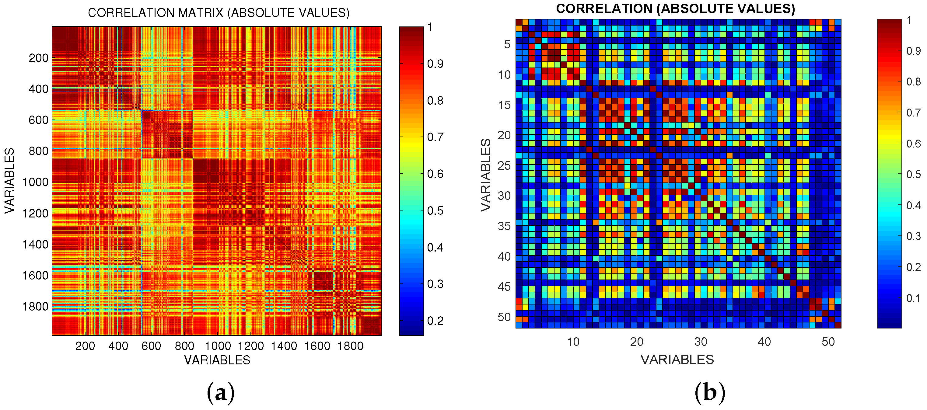
Semiconductor: In the semiconductor manufacturing industry, virtual metrology refers to the use of models to predict “costly to measure” key physical variables from more accessible in-line measurements [52]. In this case, differently from the previous Section 5.1, we have a real target output (not built artificially): the plasma etch rate (ER) during the production of silicon wafers [53]. The in-line measurements are obtained from optical emission spectroscopy data consisting of specific wavelengths from which statistical moments (mean, variance, skewness, etc.) are calculated. We recast the prediction of ER into a classification problem with the aim of classifying out-of-spec ER measurements (outside reference values) and identify input variables that help to identify these events. In order to deal with the potentially high number of features extracted from the data (each statistical moment is calculated for each wavelength), only features presenting a reasonably good correlation with ER are used as candidate variables to build the models. This dataset presents high collinearity among subsets of variables as can be seen from Figure 2a.

(IV)

Arcene’s task is to distinguish cancer versus normal patterns from mass-spectrometric data. This is a two-class classification problem with continuous input variables.

(V)

Gisette is a handwritten digit recognition problem focused on the separation of the highly confusible digits “4” and “9”. Arcene, Gisette and Madelon dataset explained before are three of the five datasets used in the NIPS 2003 feature selection challenge.

(VI)

Fabric Care Appliance is a dataset provided by Electrolux Italia S.p.a, fabric and dish care R&D. This dataset was collected with the purpose of equipping Electrolux household heat pump tumble dryers with an on-line model to predict the dry load weight of the laundry in the first part of the cycle. Generally speaking, the laundry weight of the loaded in the drum of a laundry treatment machine is an important piece of information; laundry weight can be used to set various washing/drying cycle parameters and to optimize performances and efficiency. Unfortunately, dedicated weight sensors cannot be included in consumer laundry equipment given the related costs. For this reason, a soft sensor approach, i.e., a black-box model, could be used to estimate laundry weight based on sensors already in place in laundry treatment equipment. The goal here is to distinguish between two sets of load classes: the output is a binary vector whose value is 0 for small load classes (i.e., classes $\mathrm{I},\mathrm{II},\mathrm{III}$) and 1 for large load classes (i.e., classes $\mathrm{IV},\mathrm{V},\mathrm{VI},\mathrm{VII}$); the input is a matrix of features (variables) derived from signals available on machines using expert knowledge.

Simple features have been used to summarize the entire information inherent in all signals provided: the features chosen are for example maximum or minimum values and relative positions, means or variances, slopes or integrals in different time intervals, quantities that can be computed on-line in the dryer. This dataset shows high collinearity among two subsets of variables as can be seen in Figure 2b; features in each high correlated group come from information collected by the same physical sensor.

6. Results and Discussion

6.1. Simulated/Artificial Data

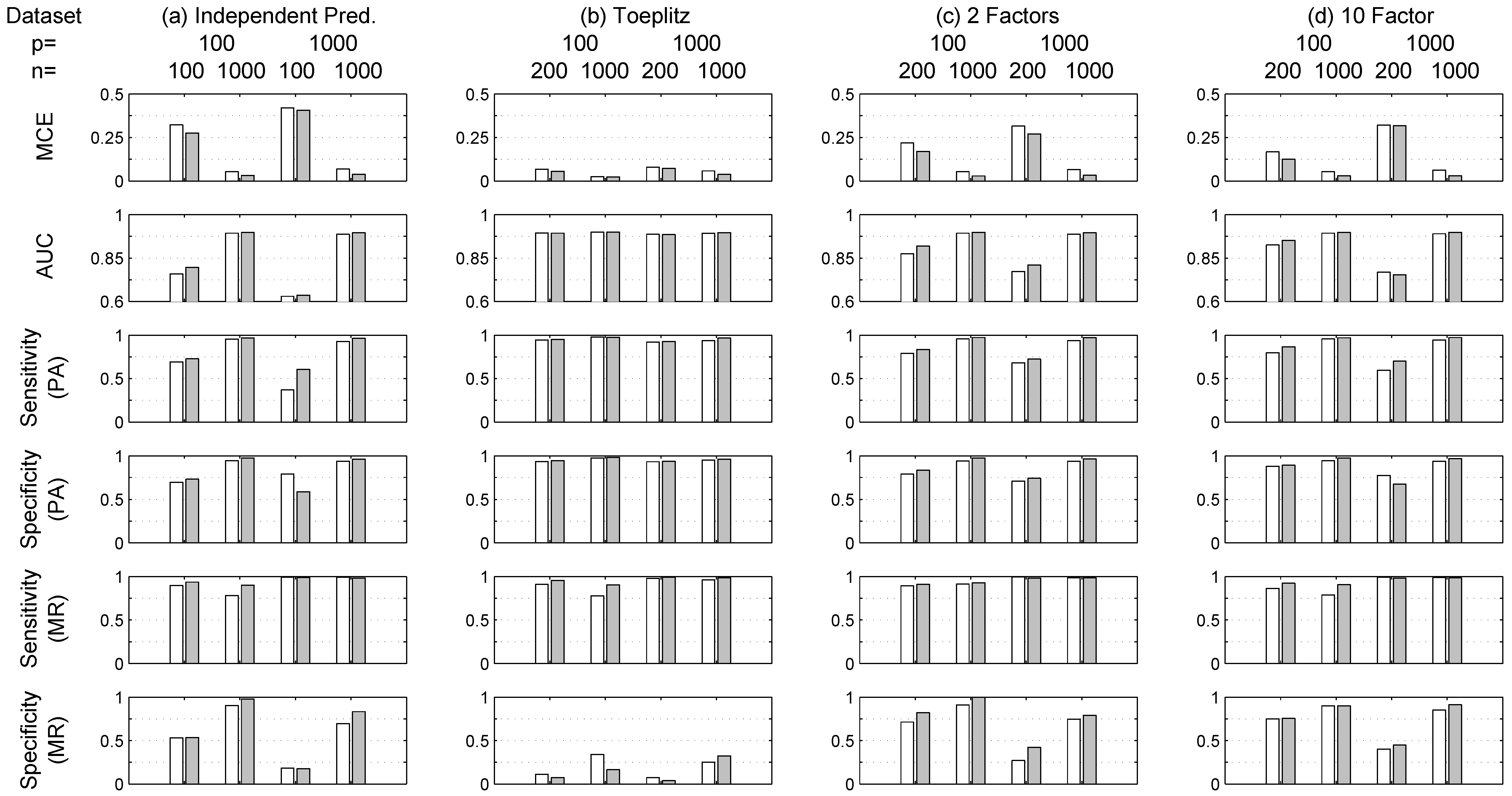
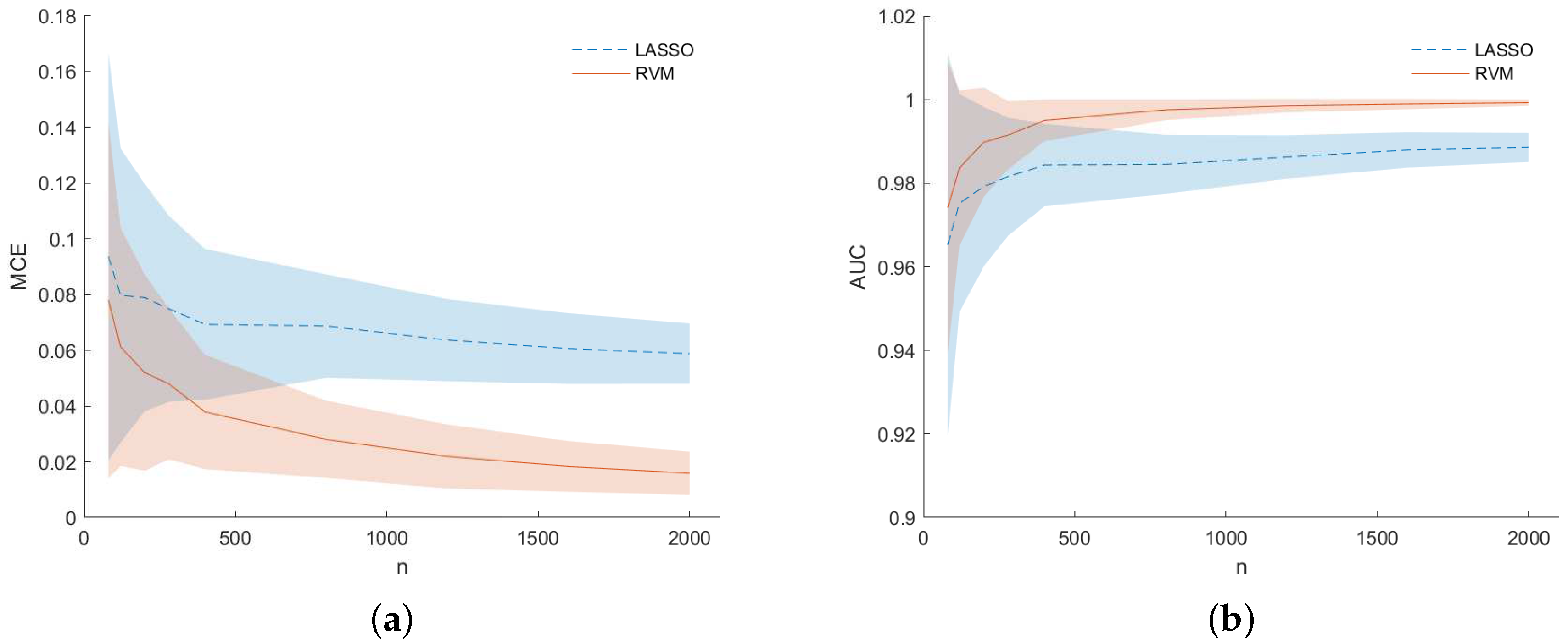
The results for the simulated datasets are presented Figure 3, Figure 4, Figure 5, Figure 6, Figure 7 and Figure 8. In particular, Figure 4, Figure 5, Figure 6, Figure 7 and Figure 8 refer to dataset (f)—Manufacturing, while Figure 3 refers to other datasets (a)–(e). As expected, in general, the performance for all indicators improves for both methods with increasing values of n, for example the MCE in Figure 5 for dataset (f) decreases as n increases. Moreover, Figure 3 shows that, in general, for the same value of n, the lower the value of p the better the performance. RVM outperforms LASSO when $p\le n$ in terms of MCE and AUC. Increasing Prediction Accuracy (PA) is obtained for both methods when p and n are comparable with respect to the case $p>>n$. For example, Figure 3 shows a drop for simulation (a) in terms of average MCE from 30% to 5% for LASSO and from 25% to 3% for RVM when $n=100$ and $n=1000$ respectively. Similar performance improvements are obtained for simulations (b)–(d) as can be seen from Figure 3. Additionally, the same figure shows that RVM tends to outperform LASSO in the estimation of the true model structure (or Model Recovery—MR) in terms of Sensitivity, i.e., True Positive rate, and Specificity, i.e., True Negative rate.

The set of simulations (e), basically the same as (a)–(d) but repeated for $p=1000$, whose results are also shown in Figure 3, confirm that RVM tends to outperform LASSO in all situations, although in a few cases results are comparable, especially when $p>>n$.

In this situation ($p>>n$), the structure discovery ability of the RVM degenerates. This can be due to the fact that the hyperparameters for RVM are optimized with an iterative procedure (see Section 3.2) that does not guarantee the cost function minimum is reached. On the other hand, the LASSO problem is convex and thus the coordinate descent algorithm is more likely to reach the minimum of the cost function.

Several studies have been conducted in the literature studying the selection consistency property of the LASSO estimator. A necessary condition for the LASSO to recover the true model structure is the so-called Irrepresentable Condition (IC) [54,55] calculated as:

$$\underset{k\in N}{max}\left|sign{\left({\mathit{\theta }}_S\right)}^T{\left({\mathbf{X}}_S^T{\mathbf{T}}_S\right)}^{-1}{\mathbf{X}}_S^T{\mathbf{X}}_k\right|<1$$

(17)

where the subscript ”S“ indicated the set of variables whose coefficients are different from zero, while N identifies the k variables with ${\theta }_k=0$. If this condition is violated, the recovery of the true model is not guaranteed.

Table 2. LASSO Irrepresentable Condition for the simulated datasets (a)–(d), (f).

Dataset	(a)				(b)				(c)
p	100		1000		100		1000		100		1000
n	100	1000	100	1000	200	1000	200	1000	200	1000	200	1000
IC	1.236	0.347	1.575	0.426	1.023	1.004	1.072	1.03	0.851	0.357	1.113	0.471
Dataset	(d)				(f)
p	100		1000		80	120	200	280	400	800	1200	1600	2000
n	200	1000	200	1000	100	1000	100	1000	100	1000	100	1000	1000
IC	0.75	0.446	0.972	0.486	2.144	2.155	2.025	2.092	2.129	2.112	2.093	2.092	2.082

collects the IC values obtained for the simulated datasets (a)–(f). Interestingly, observing Figure 3 and Table 2 it is possible to notice that the lower the IC, the higher the Specificity values in model recovery (MR) for LASSO, and specificity values are also higher for RVM when n is large. It can be also noticed that the irrepresentable condition (17) occasionally fails when the IC value is greater than 1; in these cases, the structure recovery provided by LASSO is not suitable according to (17).

With regard to LASSO, in Table 2 it can be noticed that for increasing values of n, in general, the IC value improves, i.e., is lower, even though condition (17) is not satisfied for several cases in which the LASSO structure recovery capability fails. It is pointed out that several approaches exist in the literature as alternatives to LASSO with regard to model recoveries, such as the smoothly clipped absolute deviation (SCAD) and the adaptive lasso [29], but they are not used here in order to keep the focus on the two methods mentioned: LASSO and RVM, whose variable selection capabilities are embedded within the logistic model estimation phase.

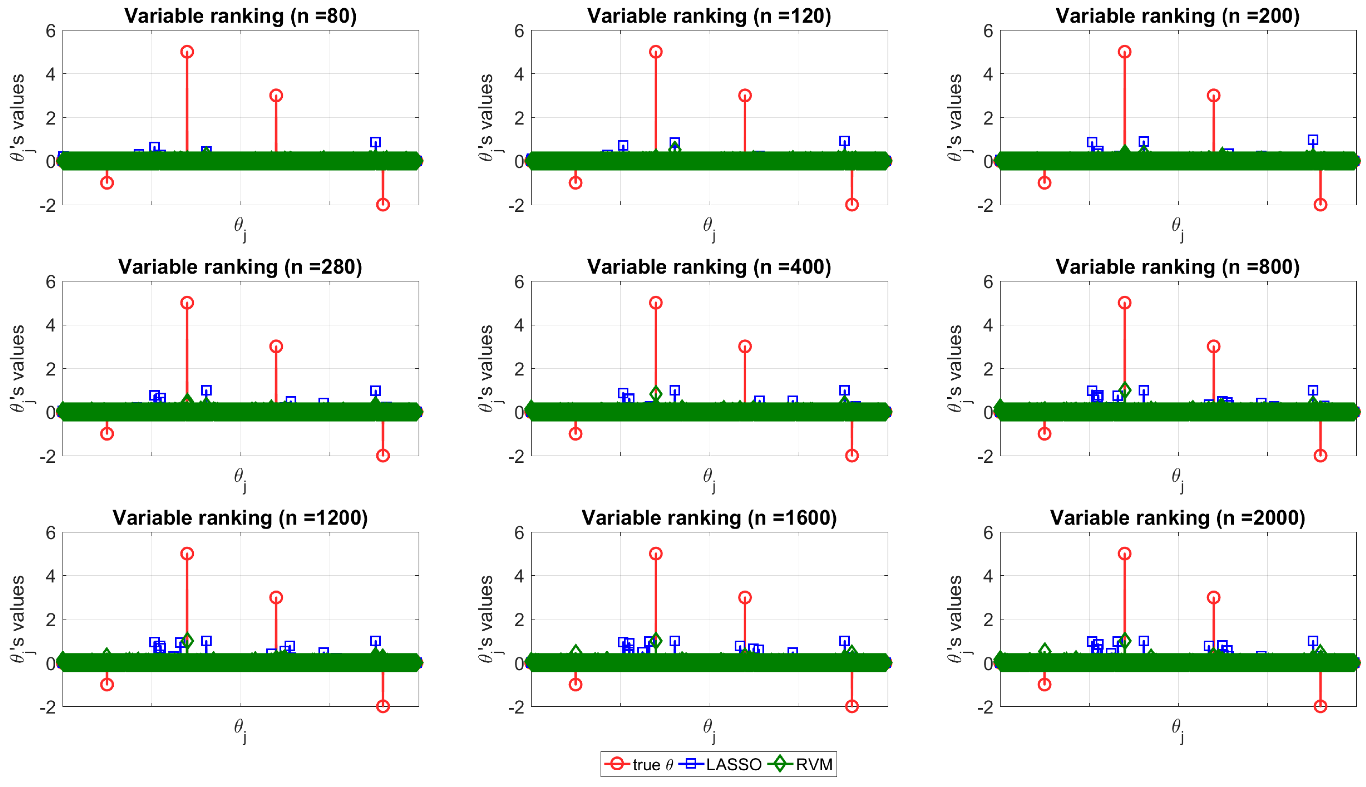
The structure discovery ability of the two techniques is depicted in Figure 4 for dataset (f), where the true vector $\theta$ (red circle) is compared with the normalized distribution obtained with the MC simulation with LASSO (blue square) and RVM (green diamond) for increasing values of n (from top left to bottom right). Figure 4 can be used to appreciate the capability of each of the two techniques in terms of structure recovery in a specific case study (dataset (f)). In this case, the predictors with more impact on the model are known in advance and are depicted in red (circle) in the figure. In this scenario, one method is better than the other if its estimates tend to overlap the real coefficient, i.e., if the stem plots of the real coefficients and estimates show nonzero values for the same indices. It can be seen that, neither RVM, nor LASSO are able to reveal the correct predictors when n is small, instead, as n increases, both of the methods tend to provide more reliable coefficients as expected.

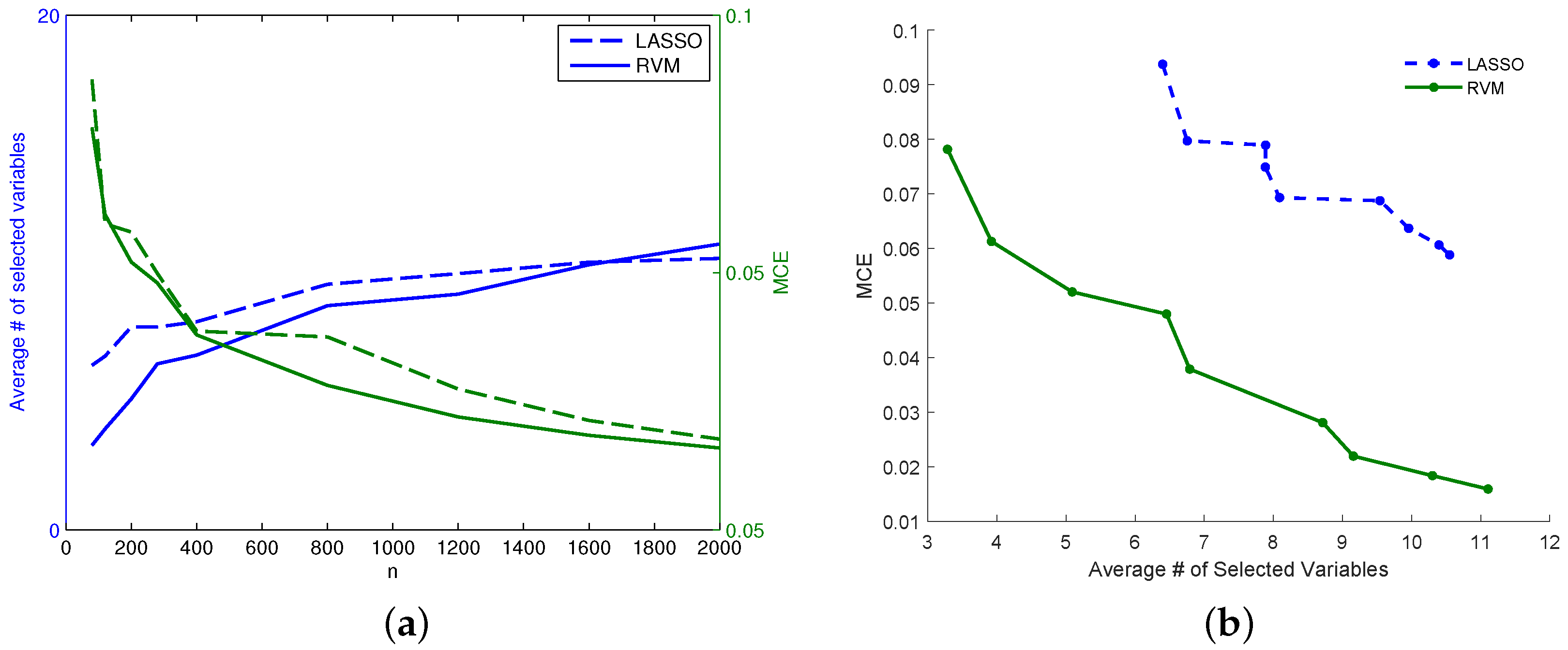
The important fact observed and pointed out here is that RVM seems to be more powerful for model recovery than LASSO when n is large, because when it shows nonzero coefficients, they match the real ones. In order to improve the readability of the picture, the reader can consider it together with

Table 3. Matches in percentage with the real indices of variables selected by LASSO and RVM for dataset (f).

n	LASSO	RVM
	Matches (%)	Matches (%)
80	25	75
200	25	75
400	25	75
1200	50	100
2000	25	100

and Figure 8a which show the same conclusions for the same data quantifying the differences. In particular, Figure 8a represents how the number of selected (nonzero) variables tends to be lower for RVM as n increases. On the other hand, Table 3 shows the matches between the selected variables and the real ones in percentage for each method. RVM appears more effective for model recovery in this case study; nevertheless, it is noteworthy to consider that this dataset presents high collinearity among variables, as already stated, and LASSO suffers somewhat from the multi-collinearity problem [33]. It turns out that, for increasing values of n, the RVM performs better than LASSO identifying the true ${\theta }_j\ne 0$, namely those that are used to predict the output class.

Considering Table 2, the reader can notice that the LASSO Irrepresentable Condition fails also for increasing values of n, so it is not surprising that better results for model recovery, in this case, are obtained with the other technique.

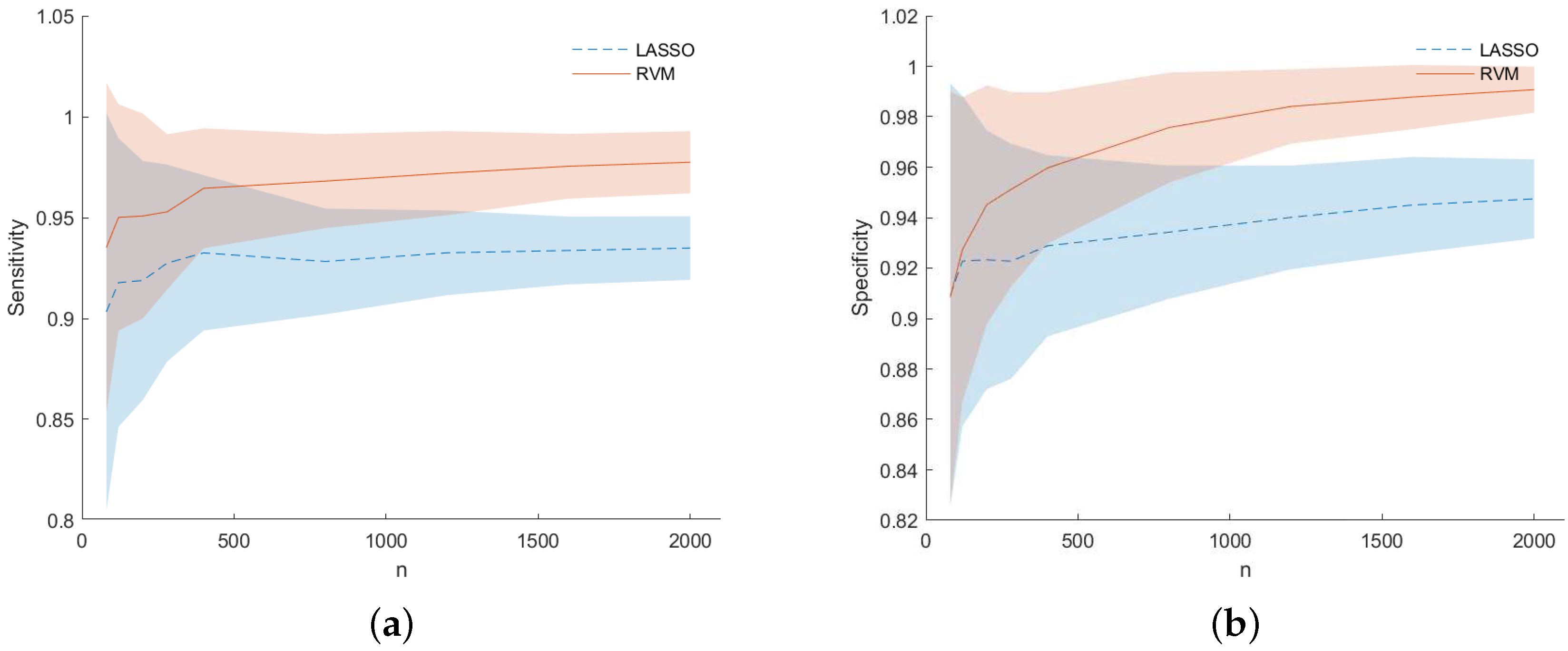
Figure 5 shows results in terms of MCE (left) and AUC (right) for dataset (f). They are presented as a function of the number of samples n used to build the dataset at each MC iteration. The RVM models (solid line) outperform the LASSO one (dashed line) as n increases to a value approximately equal to p. For low values of n, i.e., when $p>>n$, results for the LASSO and RVM became comparable as happened for simulations (b) in Figure 3. However, analyzing Figure 6 for dataset (f), one can see that RVM still outperforms the LASSO in terms of sensitivity (left) and specificity (right) for prediction accuracy (PA) considering the predicted output for the two models during the MC simulation.

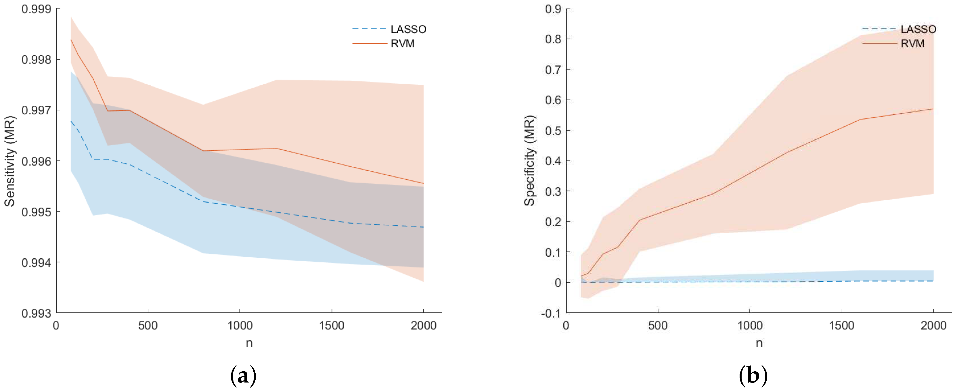
Figure 7 shows for dataset (f) the TP (or sensitivity) and TN (or specificity) rates for the model recovery capability of the two studied models. Not only LASSO often selects the wrong variables, but the selected variables are spread around the true ones (observing Figure 7 together with Figure 4). This is an example of the so-called grouping effect affecting the LASSO, namely, if there is a group of highly correlated variables, LASSO tends to select only one of them from the group and does not care which one is selected. The data under analysis are actually highly correlated in some occasions as can be seen from Figure 2 which shows the heat-map matrix of the absolute correlations between the OES dataset variables (dataset (f)). As can be seen from Figure 8 for dataset (f), while for the lower n RVM selects fewer variables than LASSO, the situation changes for increasing values of n. Despite this behavior in the sparsity of the two models, the RVM model still outperforms the LASSO in terms of MCE (continuous decreasing line in Figure 8a compared with dashed decreasing line). In particular, Figure 8b for dataset (f) shows that for an equal number of active variables in the two models, RVM achieves better prediction performance.

6.2. Real Data

Results for the real datasets are presented only in terms of prediction accuracy since the true underlying model is unknown.

Table 4. Mean and standard deviation of the MCE and the AUC distributions obtained from the MC analysis for real datasets. The lower the MCE and the higher the AUC values the better in term of accuracy.

	MCE		AUC
	LASSO	RVM	LASSO	RVM
SAheart	0.32 ± 0.05	0.30 ± 0.04	0.75 ± 0.05	0.77 ± 0.04
Abalone	0.28 ± 0.12	0.24 ± 0.11	0.81 ± 0.12	0.82 ± 0.12
Semiconductor	0.24 ± 0.02	0.21 ± 0.02	0.82 ± 0.05	0.87 ± 0.02
Arcene	0.26 ± 0.06	0.24 ± 0.06	0.82 ± 0.06	0.81 ± 0.06
Madelon	0.38 ± 0.01	0.39 ± 0.01	0.63 ± 0.01	0.64 ± 0.01
Gisette	0.04 ± 0.00	0.07 ± 0.07	0.99 ± 0.00	$0.96\pm$0.08
Fabric Care Appliance	0.03 ± 0.02	0.04 ± 0.02	0.99 ± 0.01	$0.98\pm$0.01

shows that, in general, as regards prediction accuracy, RVM and LASSO are numerically equivalent, i.e., there is no absolute winner in terms of MCE and AUC. Some considerations could be made on results considering Table 4, Figure 1 and the prior knowledge on available data, in particular:

• RVM tends to be better as n increases (and the ratio $\frac{n}{p}$ is far from 1);
• The Madelon dataset is known to be highly non-linear and dataset Fabric Care Appliance is a further example of a non-linear dataset. This leads to suggest the use of LASSO if, somehow, the non-linear structure of data is known in advance for the problem at hand; however, this consideration should be supported by other similar cases;
• The Gisette dataset is very noisy and this is due to the intrinsic difficulty of separating the digits “4” and “9”; also in this case LASSO turns out to be better than RVM;
• For the Arcene dataset where $p>>n$, RVM slightly outperforms LASSO in terms of MCE, but LASSO is better in terms of AUC.

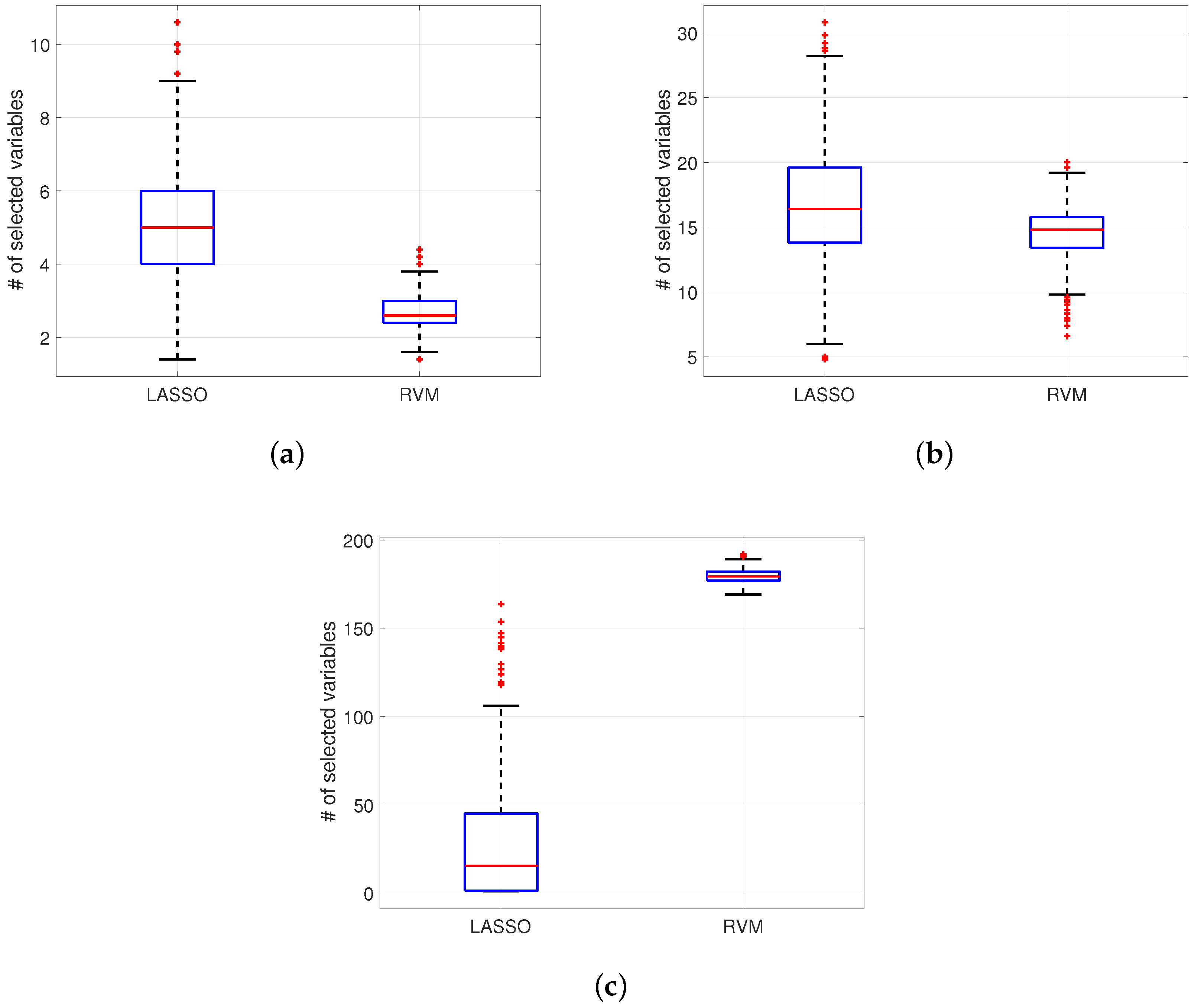
Concerning the structure recovery of the two algorithms using real datasets, some examples are depicted in Figure 9. With the Semiconductor dataset in Figure 9a RVM gives a distribution of nonzero variables in cross-validations which is less than the one provided by LASSO (for example the mean is $2.69$ for RVM and $4.99$ for LASSO). The same situation, applies for the Arcene dataset (Figure 9b) where $p>>n$, i.e., $14.63$ mean for RVM and $16.81$ for LASSO. In contrast, for the highly nonlinear dataset Madelon in Figure 9c, the difference between the mean number of selected variables in cross-validations is much higher with RVM than with LASSO ($179.58$ versus $26.92$). As a result, the use of LASSO can be recommended in general when dataset is non-linear (or even more when there is no a priori knowledge about the structure).

For real data case the same set of implementation details was kept, i.e., in terms of number of Cross-Validation, percentage of training and test data, etc. (as explained in Section 6.1).

6.3. Computational Considerations

Both implementations of the linear logistic model considered in this work are based on iterative algorithms. Thus, the time required for model parameter estimation depends on thresholds and the number of iterations specified by the user.

The update of parameters in the RVM implementation requires the inversion of a matrix to compute the posterior weight covariance matrix, an operation with complexity $\mathcal{O}\left(p^3\right)$ and memory requirement $\mathcal{O}\left(p^2\right)$ ([33,42]). The algorithm implementation described in [44] does not start by including all variables in the model but rather incrementally adds or deletes variables as appropriate. Moreover, as already noted, complexity is automatically determined.

The LASSO algorithm consists of several steps. The coordinate descent algorithm requires $\mathcal{O}\left(pn\right)$ ([33]), but additional complexity is due to the calculation of the quadratic approximation by the Newton algorithm.

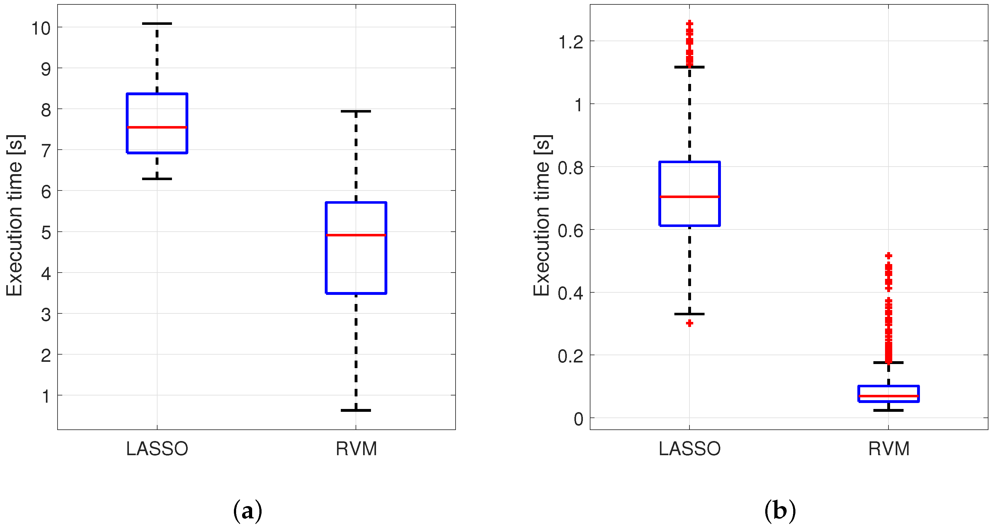
An example of comparison in terms of execution time performance has been provided in Figure 10 for 2 real cases introduced before: Arcene, and Fabric Care Appliance. These two case studies have been chosen in this case among all the others because of their $\frac{n}{p}$ ratio which is very different from one to other.

Figure 10 shows distributions of the execution times obtained for each MCCV iteration for each method. The elapsed time for each execution was measured by using tic-toc command available in MATLAB. This couple of instructions was used to tag the beginning and the end of the key code for each method so that the difference in time between the two tags indicates the desired execution time. More specifically, the tic function records the current time, and the toc function uses the recorded value to calculate the elapsed time (source: https://www.mathworks.com/help/matlab/ref/tic.html). The main steps related to the implementation of the two procedures have been summarized in

Table 5. Main steps of the implementations of the two procedures at hand in this paper. Such steps are directly involved in the running-time comparison.

	Main Steps	LASSO	RVM
I	regularization path computation	✓
II	extract model coefficients	✓	✓
III	predict test data	✓	✓

for the sake of clarity. These steps affect the execution time and are useful to stress the methodological differences between the two strategies as well. As the reader can notice, only LASSO performs the choice of the optimal regularization parameter with a dedicated inner procedure that turns out to be particularly demanding considering the entire set of iterations. On the other hand, RVM determines the model complexity automatically by the data through ARD as already stated in Section 3.2.

Step I in Table 5 refers to the code used in the glmnet LASSO implementation to determine the optimal regularization parameter lambda at a grid of values via Coordinate Descent algorithm. This part is obtained in LASSO with a nested loop (another cross-validation level for LASSO) while II provides the coefficients using the best hyperparameters fixed at the previous step.

Figure 10 shows that RVM provides an advantage in terms of execution time and this is mainly due to the fact that it does not require the estimation of a regularization parameter like LASSO. In terms of the entire code, it turns out that, for the latter, the computational effort is higher (quoted values were obtained on an Intel Core i7-4510U CPU @ 2.60GHz under Windows 10).

7. Conclusions

Increasingly high dimensional datasets are encountered in different fields of science and engineering. To handle such datasets effectively techniques are required to integrate variable selection with model building capabilities in a robust and efficient manner. In particular, it is often interesting to identify the key variables driving output variation.

This work is focused on a comparison between two sparse techniques that are well established in the literature but which have not, to date, been subject to a comprehensive comparison on several datasets with different characteristics; therefore, the aim here was to provide a reference and a tutorial for such a comparison in terms of implementation differences, performance and structure recovery. The first method, the LASSO, encodes the sparsity in the cost function and is based on regularization. The second method, RVM, encodes sparsity by setting priors over model coefficients and is based on a Bayesian implementation of the logistic model.

As regards prediction accuracy and for each setting considered in the simulation study, results showed that:

• in general RVM and LASSO appear equivalent in terms of prediction accuracy. Experimental evidence shows that RVM turns out to be better as n increases: $\frac{n}{p}$ is far from 1;
• when data is known to be strongly non-linear, as for example is the case with the Madelon dataset, LASSO shows comparable or slightly better prediction accuracy; this conclusion should be confirmed by investigating other similar highly non-linear datasets.

Concerning model recovery:

• when $p\le n$ RVM tends to outperform the LASSO;
• when $p>>n$ the situation changes. In this case, the smaller the $n/p$ ratio becomes, the more LASSO seems to identify the true underlying structure.

For the latter case, the reason can be due to the approximation procedure used to estimate the unknown quantities, i.e., model parameters, and hyperparameters, of the RVM model which suffers from large values of p. As explained in Section 3.2, the RVM implementation of the logistic model resembles an Expectation-Maximization like algorithm ([33]), where all the unknowns are iteratively updated. Large values of p make such an algorithm more sensitive to local minima of the cost function leading to possible suboptimal model parameter estimation.

Considering the experimental evidence of this study, our recommendation in accord with other results from similar works in the literature (such as [40]), is the use of LASSO when the available dataset is not sufficiently large or there is no a priori knowledge on its structure; on such occasions RVM could provide unstable predictions.

Both for prediction performances and structure recovery, the choice for the most suitable sparse learner depends on the case highlighted by the ratio $\frac{n}{p}$ as reported above.

As a final observation, RVM does not require the estimation of a regularization parameter. This could be an advantage since a completely data-driven approach is less computationally expensive and less user-subjective. On the other hand, the manual setting of the complexity parameter for the LASSO can be useful when there is a need to tailor the model complexity to the specific problem under analysis.

Despite the widespread popularity of the LASSO algorithm in the last decade, with this work, we have shown that RVM deserves more attention as a candidate technique for the estimation of sparse models. Not only it is competitive in terms of classification prediction accuracy and model recovery when compared to the LASSO, but it also does not have the overhead of a cross-validation procedure for complexity parameter tuning.

References

- Wu, T.T.; Chen, Y.F.; Hastie, T.; Sobel, E.; Lange, K. Genome-wide association analysis by lasso penalized logistic regression. Bioinformatics 2009, 25, 714–721. [Google Scholar] [CrossRef] [PubMed]
- Cenedese, A.; Susto, G.A.; Belgioioso, G.; Cirillo, G.I.; Fraccaroli, F. Home Automation Oriented Gesture Classification From Inertial Measurements. IEEE Trans. Autom. Sci. Eng. 2015, 12, 1200–1210. [Google Scholar] [CrossRef]
- Pampuri, S.; Schirru, A.; Susto, G.A.; De Luca, C.; Beghi, A.; De Nicolao, G. Multistep virtual metrology approaches for semiconductor manufacturing processes. In Proceedings of the 2012 IEEE International Conference on Automation Science and Engineering (CASE), Seoul, Korea, 20–24 August 2012; pp. 91–96. [Google Scholar]
- Susto, G.A.; Beghi, A.; De Luca, C. A virtual metrology system for predicting cvd thickness with equipment variables and qualitative clustering. In Proceedings of the ETFA2011, Toulouse, France, 5–9 September 2011; pp. 1–4. [Google Scholar]
- Dall’Anese, E.; Bazerque, J.A.; Giannakis, G.B. Group sparse Lasso for cognitive network sensing robust to model uncertainties and outliers. Phys. Commun. 2012, 5, 161–172. [Google Scholar] [CrossRef]
- Hu, X.; Tang, L.; Tang, J.; Liu, H. Exploiting social relations for sentiment analysis in microblogging. In Proceedings of the Sixth ACM International Conference on Web Search and Data Mining (2013), Rome, Italy, 4–8 February 2013; pp. 537–546. [Google Scholar]
- Lampos, V.; Cristianini, N. Tracking the flu pandemic by monitoring the social web. In Proceedings of the 2010 2nd International Workshop on Cognitive Information Processing (CIP), Elba Island, Italy, 14–16 June 2010; pp. 411–416. [Google Scholar]
- Saeys, Y.; Inza, I.; Larrañaga, P. A review of feature selection techniques in bioinformatics. Bioinformatics 2007, 23, 2507–2517. [Google Scholar] [CrossRef] [PubMed] [Green Version]
- Inza, I.; Larrañaga, P.; Blanco, R.; Cerrolaza, A.J. Filter versus wrapper gene selection approaches in DNA microarray domains. Artif. Intell. Med. 2004, 31, 91–103. [Google Scholar] [CrossRef]
- Dash, M.; Liu, H. Feature selection for classification. Intell. Data Anal. 1997, 1, 131–156. [Google Scholar] [CrossRef]
- Guyon, I.; Elisseeff, A. An introduction to variable and feature selection. J. Mach. Learn. Res. 2003, 3, 1157–1182. [Google Scholar]
- Tibshirani, R. Regression shrinkage and selection via the lasso. J. R. Stat. Soc. Ser. B (Methodol.) 1996, 58, 267–288. [Google Scholar] [CrossRef]
- Chen, S.S.; Donoho, D.L.; Saunders, M.A. Atomic decomposition by basis pursuit. Siam J. Sci. Comput. 1998, 20, 33–61. [Google Scholar] [CrossRef]
- Zou, H.; Hastie, T. Regularization and variable selection via the elastic net. J. R. Stat. Soc. Ser. (Stat. Methodol. 2005, 67, 301–320. [Google Scholar] [CrossRef] [Green Version]
- Tipping, M.E. Sparse Bayesian Learning and the Relevance Vector Machine. J. Mach. Learn. Res. 2001, 1, 211–244. [Google Scholar]
- Shalev-Shwartz, S.; Zhang, T. Accelerated proximal stochastic dual coordinate ascent for regularized loss minimization. In Proceedings of the International Conference on Machine Learning, Bejing, China, 22–24 June 2014; pp. 64–72. [Google Scholar]
- Yuan, G.X.; Ho, C.H.; Lin, C.J. An improved glmnet for l1-regularized logistic regression. J. Mach. Learn. Res. 2012, 13, 1999–2030. [Google Scholar]
- Yuan, G.X.; Chang, K.W.; Hsieh, C.J.; Lin, C.J. A comparison of optimization methods and software for large-scale l1-regularized linear classification. J. Mach. Learn. Res. 2010, 11, 3183–3234. [Google Scholar]
- Schmidt, M.; Fung, G.; Rosales, R. Fast optimization methods for l1 regularization: A comparative study and two new approaches. In Machine Learning: ECML 2007; Springer: Berlin, Germany, 2007; pp. 286–297. [Google Scholar]
- Zanon, M.; Susto, G.A.; McLoone, S. Root cause analysis by a combined sparse classification and Monte 558 Carlo approach. IFAC Proc. Vol. 2014, 47, 1947–1952. [Google Scholar] [CrossRef] [Green Version]
- Roth, V. The generalized LASSO. IEEE Trans. Neural Netw. 2004, 15, 16–28. [Google Scholar] [CrossRef] [PubMed]
- Osborne, M.R.; Presnell, B.; Turlach, B.A. On the lasso and its dual. J. Comput. Graph. Stat. 2000, 9, 319–337. [Google Scholar]
- Gao, J.; Kwan, P.W.; Shi, D. Sparse kernel learning with LASSO and Bayesian inference algorithm. Neural Netw. 2010, 23, 257–264. [Google Scholar] [CrossRef]
- Janusz, A.; Grzegorowski, M.; Michalak, M.; Wrobel, L.; Sikora, M.; Ślęzak, D. Predicting seismic events in coal mines based on underground sensor measurements. Eng. Appl. Artif. Intell. 2017, 64, 83–94. [Google Scholar] [CrossRef]
- Bühlmann, P.; Hothorn, T. Boosting algorithms: Regularization, prediction and model fitting. Stat. Sci. 2007, 22, 477–505. [Google Scholar] [CrossRef]
- Schapire, R.E. The boosting approach to machine learning: An overview. In Nonlinear Estimation and Classification; Springer: Berlin, Germany, 2003; pp. 149–171. [Google Scholar]
- Freund, Y.; Schapire, R.E. A decision-theoretic generalization of on-line learning and an application to boosting. J. Comput. Syst. Sci. 1997, 55, 119–139. [Google Scholar] [CrossRef] [Green Version]
- Freund, Y.; Schapire, R.E. Experiments with a new boosting algorithm. ICML Citeseer 1996, 96, 148–156. [Google Scholar]
- Zou, H. The adaptive lasso and its oracle properties. J. Am. Stat. Assoc. 2006, 101, 1418–1429. [Google Scholar] [CrossRef] [Green Version]
- Huang, J.; Ma, S.; Zhang, C.H. Adaptive Lasso for sparse high-dimensional regression models. Stat. Sin. 2008, 18, 1603–1618. [Google Scholar]
- Collins, M.; Schapire, R.E.; Singer, Y. Logistic regression, AdaBoost and Bregman distances. Mach. Learn. 2002, 48, 253–285. [Google Scholar] [CrossRef]
- Bauschke, H.H.; Borwein, J.M. Joint and separate convexity of the Bregman distance. In Studies in Computational Mathematics; Elsevier: Amsterdam, The Netherlands, 2001; Volume 8, pp. 23–36. [Google Scholar]
- Friedman, J.; Hastie, T.; Tibshirani, R. The Elements of Statistical Learning; Number 10; Springer: New York, NY, USA, 2001. [Google Scholar]
- Bühlmann, P.; Yu, B. Boosting with the L 2 loss: Regression and classification. J. Am. Stat. Assoc. 2003, 98, 324–339. [Google Scholar] [CrossRef]
- Friedman, J.H. Greedy function approximation: A gradient boosting machine. Ann. Stat. 2001, 29, 1189–1232. [Google Scholar] [CrossRef]
- Wu, Y.; Wipf, D.; Yun, J.M. Understanding and Evaluating Sparse Linear Discriminant Analysis. Available online: http://proceedings.mlr.press/v38/wu15.pdf (accessed on 10 May 2020).
- Welling, M. Fisher Linear Discriminant Analysis. Available online: https://www.ics.uci.edu/~welling/teaching/273ASpring09/Fisher-LDA.pdf (accessed on 10 May 2020).
- Du, Y.; Budman, H.; Duever, T.A.; Du, D. Fault Detection and Classification for Nonlinear Chemical Processes using Lasso and Gaussian Process. Ind. Eng. Chem. Res. 2018, 57, 8962–8977. [Google Scholar] [CrossRef]
- Ge, Z.; Song, Z. Nonlinear soft sensor development based on relevance vector machine. Ind. Eng. Chem. Res. 2010, 49, 8685–8693. [Google Scholar] [CrossRef]
- Urhan, A.; Alakent, B. An Exploratory Analysis of Biased Learners in Soft-Sensing Frames. arXiv 2019, arXiv:1904.10753. [Google Scholar]
- Friedman, J.; Hastie, T.; Tibshirani, R. Regularization paths for generalized linear models via coordinate descent. J. Stat. Softw. 2010, 33, 1. [Google Scholar] [CrossRef] [Green Version]
- Bertsekas, D.P.; Tsitsiklis, J.N. Parallel and Distributed Computation: Numerical Methods; Prentice Hall: Englewood Cliffs, NJ, USA, 1989; Volume 23. [Google Scholar]
- MacKay, D.J. The evidence framework applied to classification networks. Neural Comput. 1992, 4, 720–736. [Google Scholar] [CrossRef]
- Tipping, M.E.; Faul, A.C. Fast marginal likelihood maximisation for sparse Bayesian models. In Proceedings of the AISTATS, Key West, FL, USA, 3–6 January 2003. [Google Scholar]
- Fletcher, T. Relevance Vector Machines Explained; University College London: London, UK, 2010. [Google Scholar]
- MacKay, D.J. A practical Bayesian framework for backpropagation networks. Neural Comput. 1992, 4, 448–472. [Google Scholar] [CrossRef]
- Neal, R.M. Bayesian Learning for Neural Networks; Springer-Verlag New York, Inc.: Secaucus, NJ, USA, 1996. [Google Scholar]
- Picard, R.R.; Cook, R.D. Cross-validation of regression models. J. Am. Stat. Assoc. 1984, 79, 575–583. [Google Scholar] [CrossRef]
- Kuhn, M.; Johnson, K. Applied Predictive Modeling; Springer: Berlin, Germany, 2013; Volume 26. [Google Scholar]
- Kohavi, R. A study of cross-validation and bootstrap for accuracy estimation and model selection. IJCAI Montr. Can. 1995, 2, 1137–1145. [Google Scholar]
- Fisher, R.A. Statistical methods for research workers. In Breakthroughs in Statistics; Springer: Berlin, Germany, 1992; pp. 66–70. [Google Scholar]
- Susto, G.A.; Beghi, A. A virtual metrology system based on least angle regression and statistical clustering. Appl. Stoch. Model. Bus. Ind. 2013, 29, 362–376. [Google Scholar] [CrossRef]
- Schirru, A.; Susto, G.A.; Pampuri, S.; McLoone, S. Learning from time series: Supervised aggregative feature extraction. In Proceedings of the 2012 IEEE 51st IEEE Conference on Decision and Control (CDC), Maui, HI, USA, 10–13 December 2012; pp. 5254–5259. [Google Scholar]
- Meinshausen, N.; Bühlmann, P. High-dimensional graphs and variable selection with the lasso. Ann. Stat. 2006, 34, 1436–1462. [Google Scholar] [CrossRef] [Green Version]
- Zhao, P.; Yu, B. On model selection consistency of Lasso. J. Mach. Learn. Res. 2006, 7, 2541–2563. [Google Scholar]
Figure 1.
Diversity of real/artificial datasets in terms of class samples distribution and ratio.
Figure 2.
Absolute value of the correlation matrix for the semiconductor dataset (OES data) (a) and Fabric Care Appliance dataset: (b).
Figure 3.
Summary of the simulation results obtained with simulated datasets (a–d): ![Algorithms 13 00137 i002]() LASSO results;
LASSO results; ![Algorithms 13 00137 i003]() RVM results.
RVM results.
LASSO results;
LASSO results; RVM results.
Figure 4.
Coefficients estimated with LASSO (blue) and RVM (green) compared with the real ones (red) for dataset (f).
Figure 5.
dataset (f): MCE (a) and AUC (b) for LASSO (dashed) and RVM (solid). The average MCE and AUC values are represented by tick lines, while the shaded areas represent the standard deviation obtained across the MC simulation.
Figure 6.
dataset (f): Sensitivity (a) and specificity (b) as regard Prediction Accuracy (PA) for LASSO (dashed) and RVM (soid). The shaded areas represent the standard deviation obtained across the MC simulation.
Figure 7.
dataset (f): Sensitivity (a) and Specificity (b) as regard Model Recovery (MR) ability for LASSO (dashed) and RVM (solid). Shaded areas for standard deviation across the MC simulations.
Figure 8.
dataset (f): (a) Average number of selected variables (increasing lines) and MCE (decreasing lines) for LASSO (dashed) and RVM (continuous). (b) MCE for LASSO (dashed) and RVM (solid).
Figure 9.
Examples of number of selected variables for RVM and LASSO depending on MCCV iterations (1000). Semiconductor data in (a), Arcene (b) and Madelon (c).
Figure 10.
Examples of distributions of execution times in seconds for RVM and LASSO depending on MCCV iterations (1000). Arcene data in (a), and Fabric Care Appliance data (b).