Sphere Fitting with Applications to Machine Tracking


Computer Science Department, University of Haifa, 199 Aba Khoushy Ave., Mount Carmel, Haifa, P.C. 3498838, Israel
*
Author to whom correspondence should be addressed.
Algorithms 2020, 13(8), 177; https://0-doi-org.brum.beds.ac.uk/10.3390/a13080177
Submission received: 5 June 2020
/
Revised: 12 July 2020
/
Accepted: 15 July 2020
/
Published: 22 July 2020
(This article belongs to the Section Randomized, Online, and Approximation Algorithms)
Abstract
:We suggest a provable and practical approximation algorithm for fitting a set P of n points in to a sphere. Here, a sphere is represented by its center and radius . The goal is to minimize the sum of distances to the points up to a multiplicative factor of , for a given constant , over every such r and x. Our main technical result is a data summarization of the input set, called coreset, that approximates the above sum of distances on the original (big) set P for every sphere. Then, an accurate sphere can be extracted quickly via an inefficient exhaustive search from the small coreset. Most articles focus mainly on sphere identification (e.g., circles in image) rather than finding the exact match (in the sense of extent measures), and do not provide approximation guarantees. We implement our algorithm and provide extensive experimental results on both synthetic and real-world data. We then combine our algorithm in a mechanical pressure control system whose main bottleneck is tracking a falling ball. Full open source is also provided.
1. Introduction
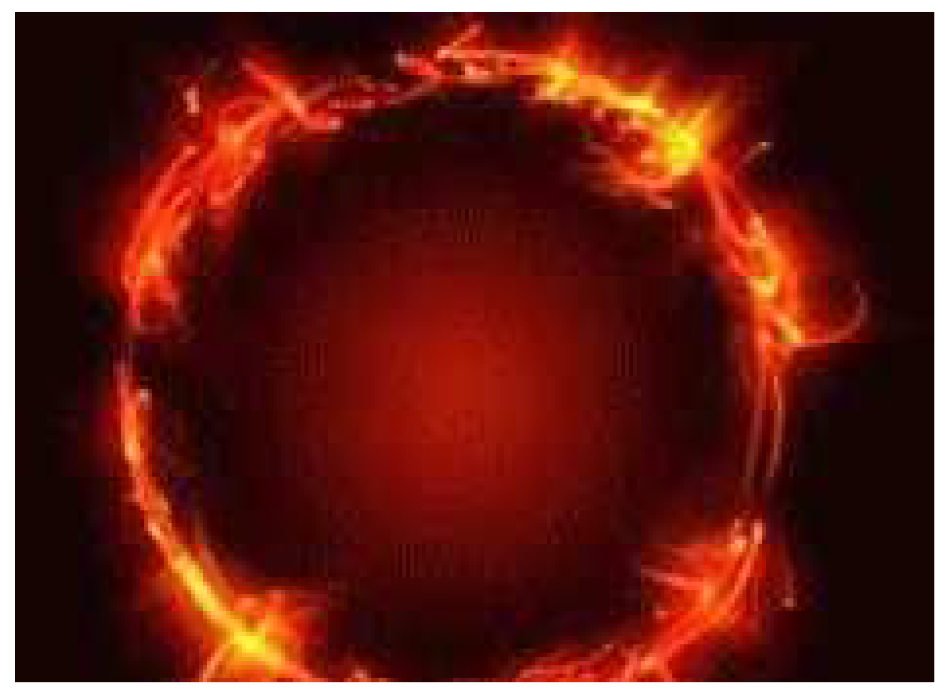
Approximating or fitting a set of points in a d-dimensional space by a simple shape is a fundamental problem in geometric optimization with many applications in robotics [1,2,3], computational geometry [4,5,6], machine learning [7,8], computer vision [9,10], image processing [11], computational metrology, etc. A tangible example is finding the exact location of the flaming ring as shown in Figure 1.
A possible model, which we use in this paper, is to minimize the sum of distances (called the -norm of the distance vectors). The sum of distances is known to be more robust to noise than the sum of squared distances. For example, the number that minimizes the sum of distances to a set of n numbers is its median, and increasing one of the input numbers to infinity would not change this solution. However, this is not the case for the mean, which minimizes the sum of squared distances. For every and we define
to be the measure function for median-sphere.
Most existing techniques are heuristics with no provable bounds on the approximation error, or have some understanding of the input points.
In this paper, we consider the special case of approximating points by a sphere, and hope to generalize the technique to other shapes in the future. Let
represent an optimal median-sphere. Our goal is to compute x and r such that
1.1. Related Work
1.1.1. Thinnest Sphere Annulus
For fitting a sphere to a set of points, the acceptable compromise is the approximation of the thinnest sphere annulus (called the -norm of the distance vectors), that minimizes maximum of distances to the input set, over every and .
The main drawback of this optimization function is sensitivity to a single point (outlier) in the input data set that may completely change the optimal solution even compared to the sum of squared distances that was discussed in the previous section.
1.1.2. Median-Sphere
A better fitting solution is the median-sphere (called the -norm of the distance vectors), that minimizes maximum of distances to the input set, over every and . Although there is a lot of work for the corresponding problem, less is known for the case.
1.1.3. Least Mean Square
Another measure is the least mean square, that minimizes sum of square of distances to the input set, over every .
1.1.4. Heuristics for Circles Detection in Images
Most significant work has been done for two Dimensional data in the context of image processing. Extensive work tends to compute circles for the purpose of object detection in images. However, most of these heuristics do no provide approximation guarantees and suitable only for .
A common heuristic to fit points to a circle is the well-known Circle Hough transform (CHT) [13]. The approach of this technique is to find imperfect instances of spheres by a voting procedure. This voting rates candidates of possible spheres (i.e., center and radius). The main drawback of this technique is its inefficient running time of complexity .
In [14], a circle detection was applied by Learning Automata (LA), which is a heuristic method to solve complex multi-modal optimization problems. The detection process is considered a multi-modal optimization problem, allowing the detection of multiple circular shapes through only one optimization procedure. The drawbacks of this algorithm is that it is designated to images.
A variant of a Hough transform algorithm, called EDCircles [15], aims to approximate points by arcs which are based on their Edge Drawing Parameter Free (EDPF). The general idea of the algorithm is to extract line segments in an image, convert them into circular arcs and then combine these arcs to detect circles, which is performed by an arc join heuristic algorithm with no approximation guarantees. Moreover, its running time is still inefficient when dealing with big data and large dimensional space (i.e., ) in the worst case.
In [16], a circle detector based on region-growing of gradient and histogram distribution of Euclidean distances is presented. Region-growing of the gradient is applied to generate arc support regions from a single point. The corresponding square fitting areas are defined to accelerate detection and decrease storage. A histogram is then used to count frequency of the distances that participates in the accumulator and the parameters of each circle are acquired.
In [17], the proposed detection method is based on geometric property and polynomial fitting in polar coordinates instead of Cartesian coordinates. It is tailored for two-dimensional LIDAR (laser radar sensors) data. They use Support Vector Machines (SVM) to detect the target circular object from natural lidar coordinates features representing segments from the image. For specific examples, they measure up to detections with execution time of milliseconds per image.
A circle detection algorithm that is based on a random sampling of isosceles triangles (ITs) is presented in [18]. This algorithm provides a distinctive probability distribution for circular shapes using a small number of iterations. Although they introduced an accurate and robust detection at sharp images, it does not handle corrupted and moving images and does not have provable guarantees.
Another variant of the Hough transform algorithm [19], called Vector Quantization (VQHT), tries to detect circles by decomposing their edges in the image into many sub-images by using Vector Quantization (VQ) algorithm. The edge points that reside in each sub-image are considered as one circle candidate group. Then the
VQHT algorithm is applied for fast circle detection.
In [20,21], a randomized iterative work-flow is suggested, which exploits geometrical properties of isophotes in the image to select the most meaningful edge pixels and to classify them in subsets of equal isophote curvature.
In [22], the authors propose a method to recognize a circular form using a geometric symmetry through a rotational scanning process.
The random sample consensus (RANSAC) algorithm introduced by Fishler and Bolles in [23] is a widely used robust estimator that has become a standard in the field of computer vision. The RANSAC algorithm proceeds as follows: Repeatedly, subsets of the input data are randomly selected, and model parameters (i.e., optimal median-sphere) fitting these subsets are computed. In the second step, the quality of the sphere is evaluated on the input data. The output of the algorithm is the sphere that has the highest match of all the spheres.
1.1.5. Coreset
One of the classical techniques in developing approximation algorithms is the extraction of “small” amount of “most relevant” information from the given data (called a coreset), and then applying traditional optimal algorithms on this extracted data which ensure provable approximation results. The exact definition of coreset changes from paper to paper.
Moreover, generic techniques enable coreset maintenance of streaming, distributed and dynamic data. A survey on coresets is given in e.g., [26,27].
In [28] the author suggests a approximation for the median-sphere that takes time for constant integer , where is a function of d.
In [29] the authors suggest -approximation for the thinnest-sphere annulus fitting in time using linearization technique and -kernel of a point set P, for every .
1.2. Coreset Definition
In this paper, a coreset for an input set of points is a weighted subset, such that the sum of distances to every given sphere from the coreset and the original input is the same, up to multiplicative factor. Here, is an error parameter, and the size of the coreset usually depends on , but not always [30].
1.3. Our Main Contribution
We suggest an algorithm that computes an -coreset for the family of spheres in for the -norm of distances. The cardinality of the coreset is . See Theorem 2 for details.
Using existing algorithms, we can then extract a -approximation to the optimal sphere of the original input in additional time. That is, the algorithm outputs -approximation for (1), i.e., a pair and such that
We highlight the strengths of the technique by implementing and testing it for different values of number n of points in the input set and for distorted and noisy input points. Our solution holds for any dimension, and provides several examples for the case of points in two and three dimensional space.
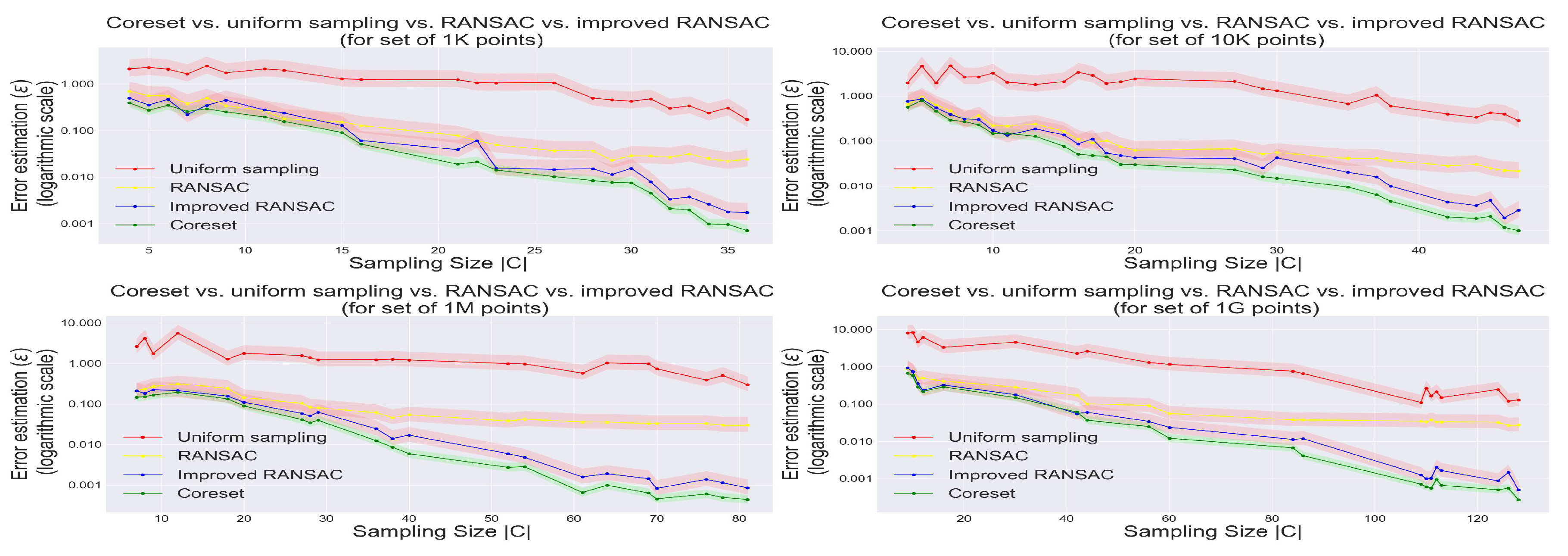
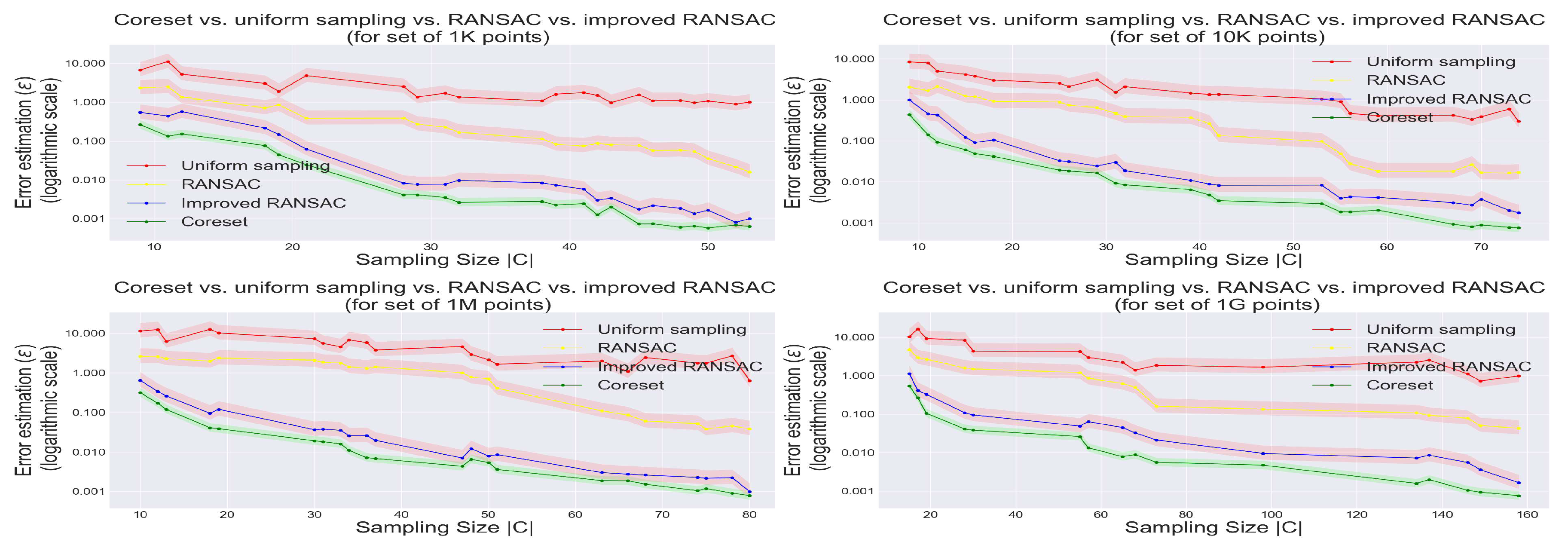
In theory, the price for using our approach is that we get only an approximated solution to the desired shape in the worst case by running the optimal solution on the coreset. In practice, we do not compute the optimal solution also on the original data, but run heuristics that search for a local minimum instead. In these cases, we see that the quality of the results on running the heuristics on the coreset is better than running them on the full large set. Intuitively, the coreset “cleans” the data, removes noise and reduces the number of bad local minima. Hence, in practice the resulting fitting error using the coreset is smaller. For example, by running the common “RANSAC” heuristic on our coreset, our experimental results show that the results are more accurate and faster; See Figure 4 in Section 3.4.
Moreover, while most of the existing solutions aim to detect a circle in two-dimensional space, our algorithm returns provable approximation for every .
As an example of a robotics application, we demonstrate our algorithms on a mechanical pressure control system which requires an efficient and extremely accurate tracking of the dynamics of a falling ball using a laser profiler, see Section 4.
1.4. Overview
In Section 2.1 we formalize the sphere fitting problem. In Section 2.3 we present and describe our shape fitting algorithms. In Section 2.4 we review the theory and the analysis of the algorithms. In Section 3 we show experimental results using our algorithm, and measures its accuracy compared to other algorithms. In Section 4 we present an operating mechanical pressure control system that uses our algorithms. In Section 5 we conclude our work and suggest open problems.
2. Methods
2.1. Median-Sphere
The median-sphere problem is to compute a sphere that best fits a given set of input points in the Euclidean d-dimensional space, i.e., a sphere that minimizes the sum of distances to these points, over every unit sphere in . For the case of two-dimensional space (i.e., points on the plane), the sphere is a circle of points on the plane.
2.1.1. Notation
For a center (point) and radius , we define sphere of radius r around x by
We denote by the union over every sphere in .
Let be a set of n points. For every , and , we define distance between p and S by
For every and a weight function , we denote the weighted sum of distances to the sphere by
Hence, smaller cost implies a better fit of the sphere to the points. For an unweighed set P, we use a default function that maps a weight of 1 to every point in P.
2.1.2. Problem Statement
Given a set P of n points in , the median-sphere is a sphere that minimizes the sum of distances to these points over every sphere in . We denote it by
We now define an -approximation to the median-sphere problem.
Definition 1
(-approx to the median-sphere). Let be a set of points, , and be a weight function. The sphere is an
α-approximation to the median-sphere if
2.2. Thinnest-Sphere
The thinnest-sphere problem is to compute a sphere that minimizes the maximum of distances to a given set of input points in the Euclidean d-dimensional space, over every unit sphere in . Formally, for a given set P of n points in , we denote the thinnest-sphere by
2.3. Algorithms
In this section we present our main algorithms. In Section 2.3.1 we present a polynomial time algorithm for computing the optimal median-sphere in time . In Section 2.3.2 we present our main algorithms for constructing an -coreset of P for sphere median. Finally, we apply the exact (inefficient) algorithm on the coreset.
2.3.1. Optimal Solution for the Median-Sphere
In order to solve the median-sphere problem we restate the problem as real polynomial system. Let , and be a sphere of radius which is centered at . Hence, is the distance between p and S. That is, if the point p is inside the sphere, and if the point p is outside the sphere. In what follows, denotes the sign of . More precisely, if , and otherwise. Therefore,
Recall that the number that minimizes the sum of distances to a set of numbers is a median of this set. Hence, is a sphere that minimizes the sum of distances to the input points, and so must separate P such that the difference between the number of points inside the sphere and the number of points outside the sphere must be less than the number of points that are placed on the sphere. That is, the number of possible permutations for constructing a set of equations (i.e., to determine a possible sign for each point) is limited by the number of spheres that can be defined using a tuple of points, i.e., spheres. Hence, we define a solution for the median-sphere problem by finding the sphere that minimizes the sum of distances to each of the polynomial systems, each consisting of n equations. The optimum among these polynomial systems is the (that is defined by its center and radius ) that minimizes the sum of distances .
In Algorithm 1, we present such algorithm for the median sphere.
Let P be a set of n points in . We denote by a tuple of different points from P. We denote by sphere the d-dimensional sphere that defined by . We denote by polynomial a system of n equations (polynomial system) that optimizes the median-sphere problem. We denote by solver an optimization for polynomial system f, e.g., using Maple [31] or Wolfram Alpha [32], etc...
| Algorithm 1: MedianSphere () |
 |
Clearly, such a solution is not applicable to a large set of points. Instead, we offer the following solution in Algorithm 2 (MedianSphereCoreset), which reduces the amount of data and then runs the existing solution on the resulting small set, called a coreset.
2.3.2. Coreset Construction
In order to reduce the number of input points, we suggest Algorithm 2 (called MedianSphereCoreset) to construct a coreset for the median sphere by removing layers of the thinnest-sphere surface using Algorithm 3 (ThinnestSphereCoreset). We first give a formal definition for such a coresets.
Definition 2
(Coreset for median-sphere). Let be a finite set of points, and be a weight function. For , , and a weight function , the pair is an ε-coreset for the median-sphere of P if for every sphere
Definition 3
(coreset for thinnest-sphere). Let be a finite set of points. A subset , is an -coresetfor the thinnest-sphere of P if for every sphere ,
For every point , we define the sensitivity [33,34] of p with respect to every sphere as its relative contribution to the overall ,
Here we assume that the sup is over every such that .
Definition 4
(Query space [35]). Let P be a finite set, be a weight function, and denote a weighted set. Let Q be a (possibly infinite) set called query set, be called a cost function, and be a function that assigns a non-negative real number for every real vector. The tuple is called a query space. For every we define the overall fitting error of to q by
The dimension of a query space is the VC-dimension of the range space that it induced, as defined below. The classic VC-dimension was defined for sets and subset and here we generalize it to query spaces, following [34].
Definition 5
It was proven in [35] that an -coreset can be obtained for a given problem (e.g., median-sphere), with high probability, by sampling points i.i.d. from the input points with respect to their sensitivity. Then we assign each sample point with a weight that is inverse proportional to its sensitivity. The number of sampled points should be proportional to the VC-dimension of the query space and the sum of sensitivities . Formally,
Theorem 1
Let be a query space of dimension , and let n be the size of P. Let be a sensitivity function for every , and let be the total sensitivity of the set P. Let . Let be a universal constant that can be determined from the proof [35]. Let
There is an algorithm in [35] that outputs weighted set such that , and, with probability at least , is an ε-coreset for .
In Algorithm 2, we present such a coreset construction for the median sphere.
2.3.3. Overview of Algorithm 2
The input for Algorithm 2 is a set P of n points in , a weight function , and an error parameter . The output of the algorithm is an -coreset for median-sphere. In Line 3, we compute (iteratively) a coreset Q for thinnest-sphere of P, see Algorithm 3. In Line 5, we assign a sensitivity for every point p in Q. The sensitivity of each point depends on the iteration number in which it was selected. In Line 7, we update the set P by removing the coreset Q from P. In Lines 8–11, we sample points to obtain coreset.
| Algorithm 2: MedianSphereCoreset() |
 |
2.3.4. Overview of Algorithm 3
The input for Algorithm 3 is a set P of n points in . The output of the algorithm is a coreset of size for thinnest-sphere, as in Definition 3. The thinnest-sphere problem depends on the external sphere surface (convex hull) and the internal sphere surface (interior convex hull) that bound the set P. Since the external sphere surface and the internal sphere surface are concentric spheres, it can be proved that the thinnest-sphere defined by exactly points where at least one of the points placed on the internal sphere surface and one of the points placed on the external sphere surface. The thinnest-sphere can be computed in time using Theorem in [29].
| Algorithm 3: ThinnestSphereCoreset(P) |
 |
2.3.5. Median-Sphere Approximation
We propose an approximation algorithm to fit a sphere (i.e., median-sphere) to a set P of n points in that is performed in the following two steps: (1) Coreset construction using Algorithm 2 to reduce the original data set to few points for each measure and (2) run the optimal Algorithm 1 on the resolved small coreset, which ensures -approximation of the optimal solution.
2.4. Analysis
In this section, we analyze the algorithms of the previous section in terms of time complexity, coreset’s size and the quality of the approximation. The approximation that is states in Theorem 2 that follows is with respect to the optimal solution such that the calculated cost of our (sphere) solution is compared directly with the calculated cost of the optimal (sphere) solution.
Theorem 2.
Let P be a set of n points in . Let . Let be the output of a call to MedianSphereCoreset(), see Algorithm 2. Then, with probability at least , is an ε-coreset of P for the median-sphere. Moreover, consists of points, and can be computed in time.
Proof of Theorem 2.
Coreset’s size:
By Line 8 of Algorithm 2, the size of the coreset is .
Running time of coreset’s construction:
Algorithm 2 has two steps. In the first step the algorithm calculates the sensitivity for every point . That is, runs iterations for picking points (Algorithm 3), each in time. Therefore, the total time of the first step is time. In the second step the algorithm picks points. Hence, the running time of Algorithm 2 is .
Accuracy:
Our proof uses the technique of [37] to bounds the maximum distance of each point in P to any sphere.
Let be the total number of iterations of the “while” loop in Lines 2–7. For every integer . let (Line 3) be the output of ThinnestSphereCoreset(P) at the i-th iteration. That is, defines concentric external and internal spheres that bounds the remaining set P. Therefore, by the triangle inequality, we can bound the maximum distance from to by
Therefore, we can bound the sensitivity of every point by
where the first inequality holds since the right denominator is a subset of the left denominator, and the second inequality holds since the numerator is uphold of the denominator by definition. Hence, the total sensitivity is
where the first equality holds by Line 5 of Algorithm 2. The middle inequality refers to the size of Algorithm 3. The right equality holds by a trivial geometric sequence.
Substituting in Theorem 1 the input set P, the VC-dimension , which raised from a trivial classification (cardinality of the largest set of points that the algorithm can shatter), and the query set , yield that with probability at least , the pair is an -coreset of P for median sphere, and therefore, the size of our coreset is . □
3. Results
3.1. Hardware
We implemented Algorithms 2 and 3 from the previous section. The implementation was done in Python language [38] using the packages Numpy [39], Scipy [40] and OpenCV [41]. We ran all the tests on a standard Intel GHz CPU laptop. Open code with scripts for reproducing our experiments is provided in [42].
3.2. Software and Algorithms
We implemented the following algorithms: (1) compute an optimal solution for the median-sphere problem (1) via exhaustive search. (2) Compute such an optimal solution over a unified sampled subset of the input data set. (3) “RANSAC” algorithm that iteratively compares adjusted spheres over a small subset of points. (4) “RANSAC” algorithm applied on the coreset (called “Improved RANSAC”), which selects points using our coreset. (5) The “heuristics Least Mean Square” from “OpenCV” algorithm package [41]. (6) Compute thinnest-sphere () solution from [29]. (7) Run “OpenCV” algorithm package for circle detection [41]. (8) Compute an optimal solution over the coreset.
3.3. Data Sets
We generated synthetic data sets of dimensions . The data sets are of different sizes, and with different types of noise characteristics. We also gather some RGB images that captured rings with a flame of fire [12], that simulates noises and abnormalities.
3.4. Experiments
We run the above algorithms and compared their performance with and without our coresets for both real and synthetic datasets.
The results show that our algorithm significantly improves both the running time and accuracy of existing heuristics by applying them to the proposed coresets (“Improved RANSAC”). Of course, for the case of computing the optimal solution (via exhaustive search), the result that is extracted from the coreset cannot be better than the one from the original input. However, as expected by our analysis, the approximation error is small while the running time is shorter by orders of magnitude.
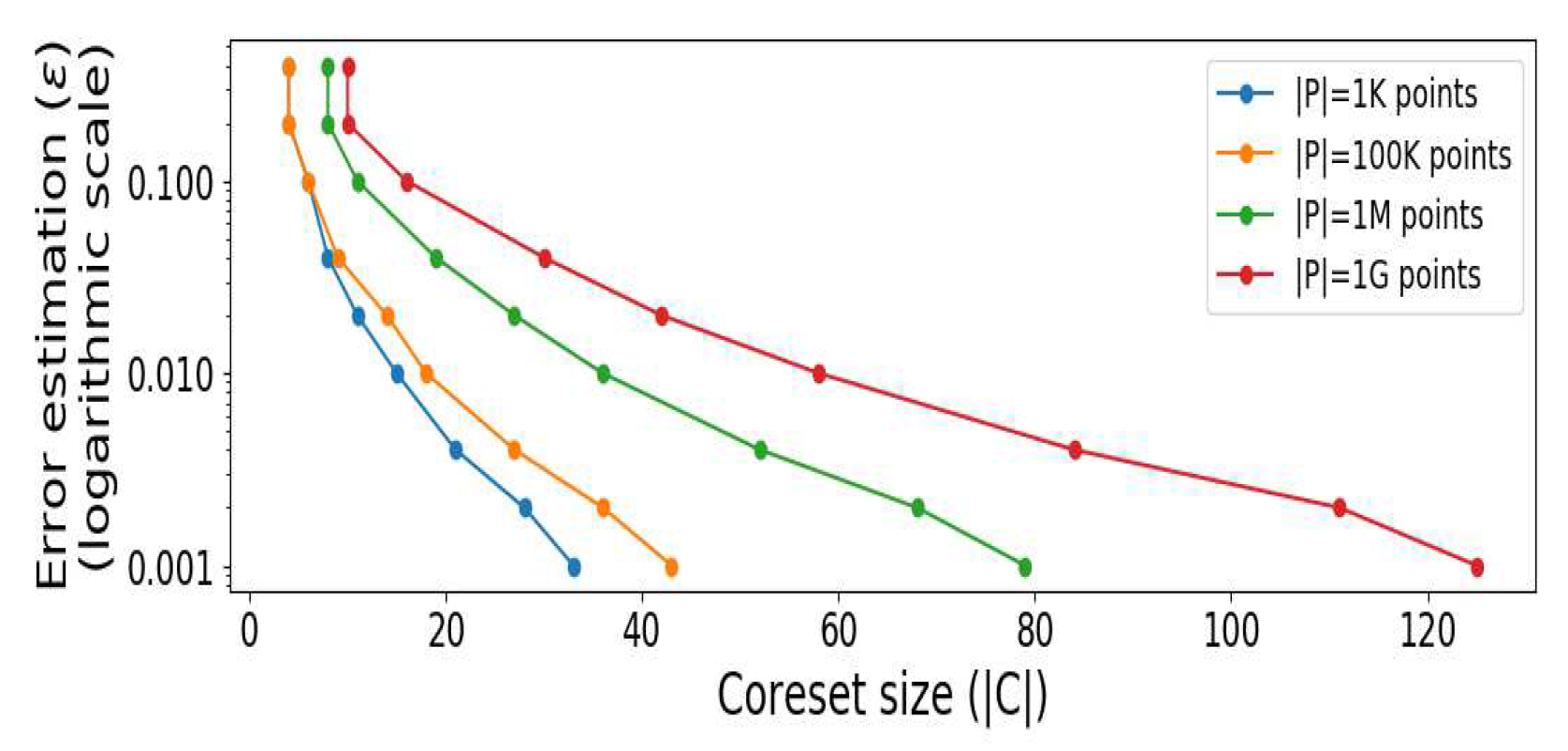
3.4.1. Coreset’S Size
The coreset size returned by Algorithm 2 is determined by the required approximation error , and dependency on the size of the origin set as required in Line 8. Examples are given in Figure 2.
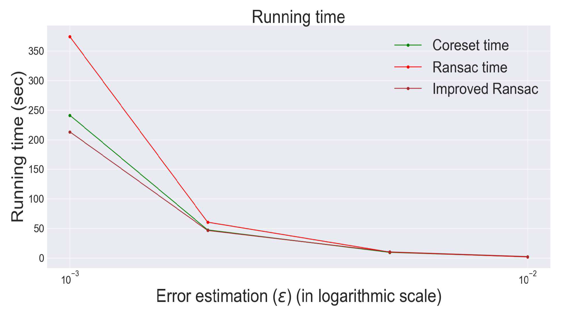
3.4.2. Running Time
Figure 3 shows that the runtime of our algorithm is far better than other algorithms, such as the “RANSAC” algorithm that considered fast. Furthermore, using our coreset algorithm to select important points significantly improves these algorithms, i.e., “Improved RANSAC”.
3.4.3. Accuracy
3.4.4. Fitting a Sphere over Images
Other visible examples allow us to show how our algorithm is able to identify and validate the “exact” circle within a set of points representing diverse images. Figure 7 shows samples of such fitting over images.
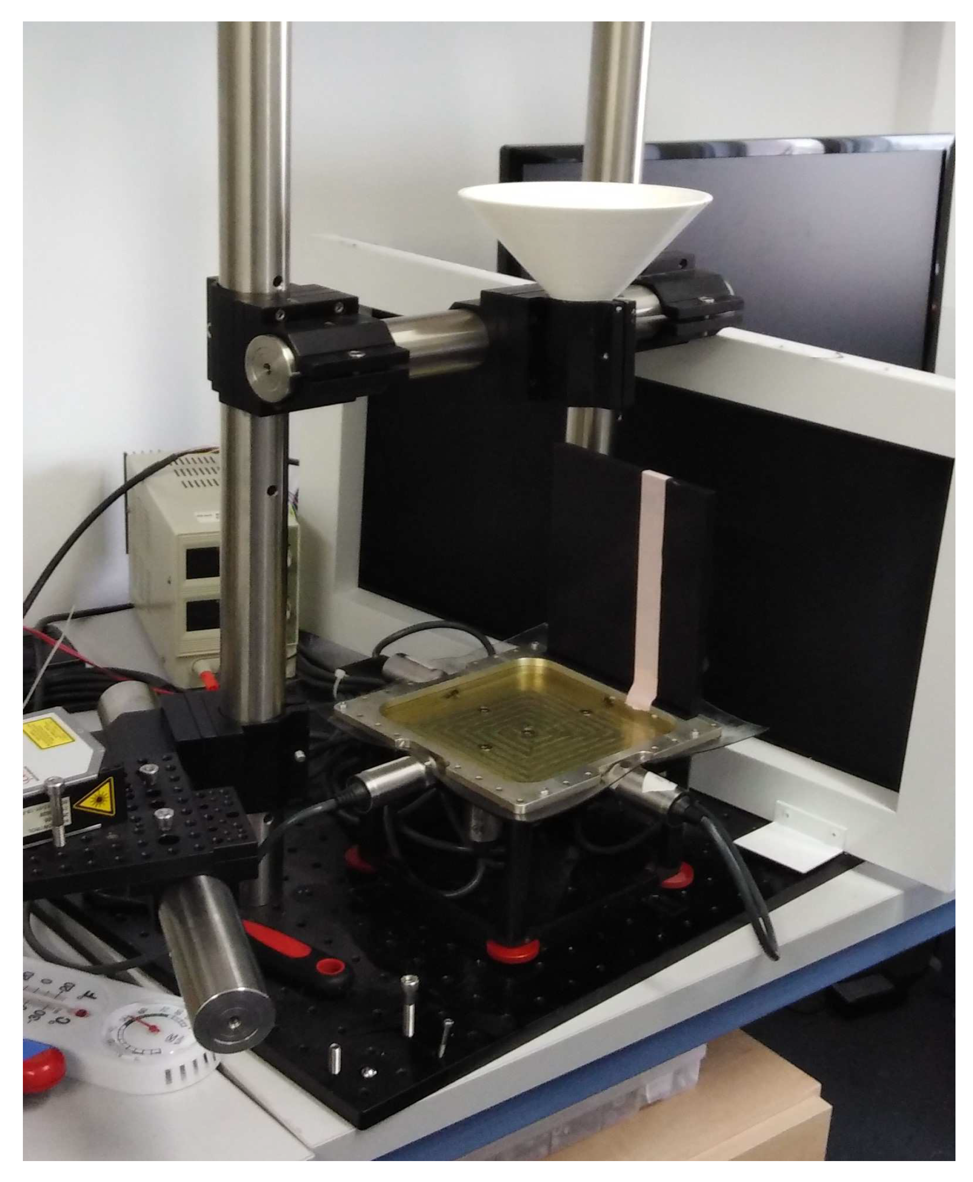
4. Example System–Mechanical Pressure Control
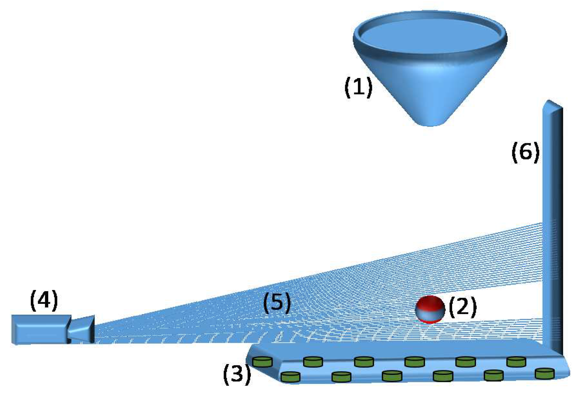
In this section, we present an experimental mechanical pressure control system that uses our coreset construction to track a falling ball; See Figure 8. The goal of the system is to learn and compare the kinetic effect on different types of materials, namely rubber membranes that consist of an aluminum layer with a thin layer of thick silicone oil. This is by using pressure sensors located below these materials, and by tracking the movement of a ball (marble) that is falling from a filter to a ground (board) that is made by one of these materials.
Comparing the path on different boards and from different heights implies the properties of each of the materials which are useful for many applications in material engineering [43,44,45].
The tracking is done via laser beams that scan the depth in each direction till hitting an object; see Figure 9. In our case, the object is either the ball (in a depth that depends on its diameter) or the white sticker behind the falling path of the ball.
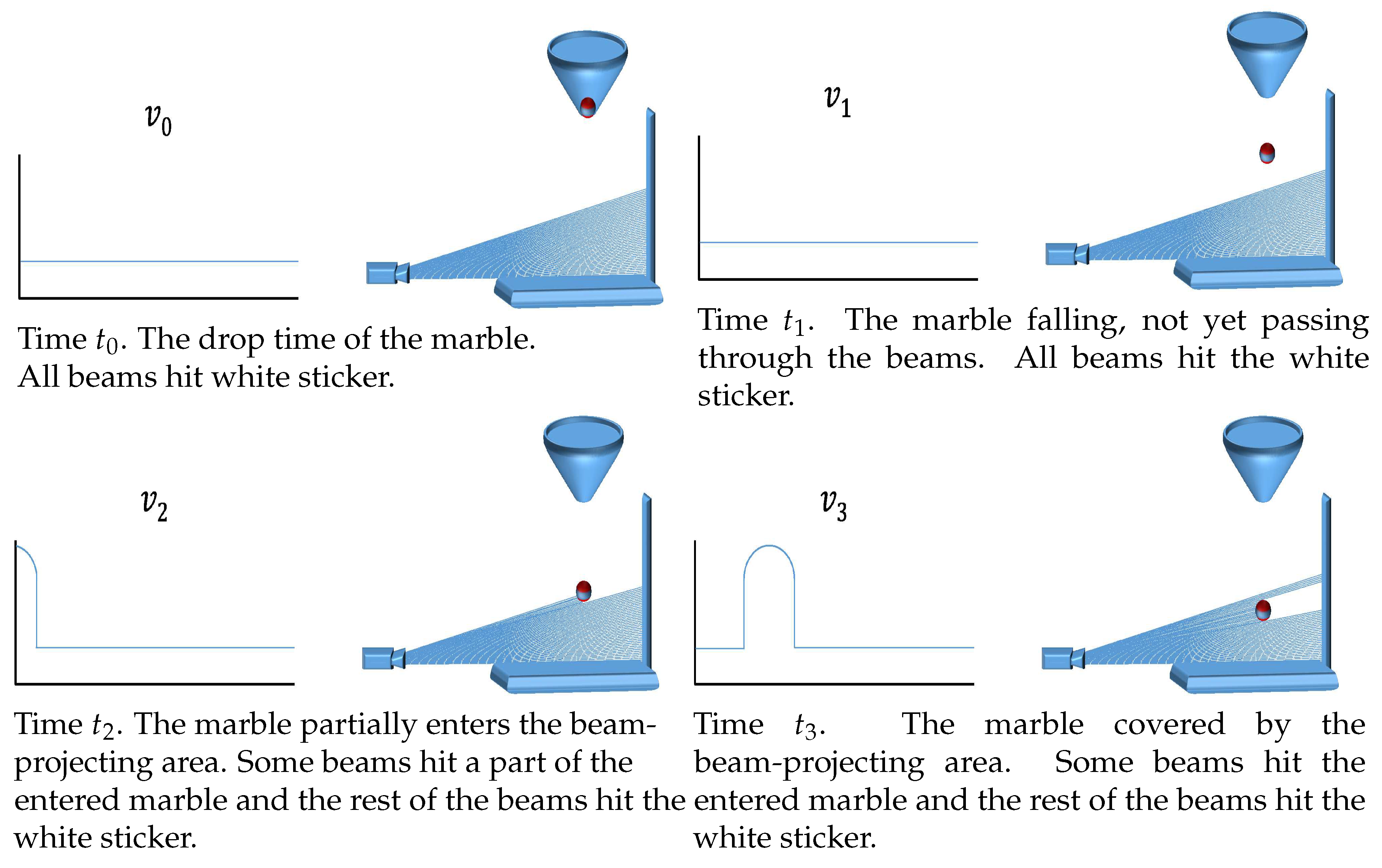
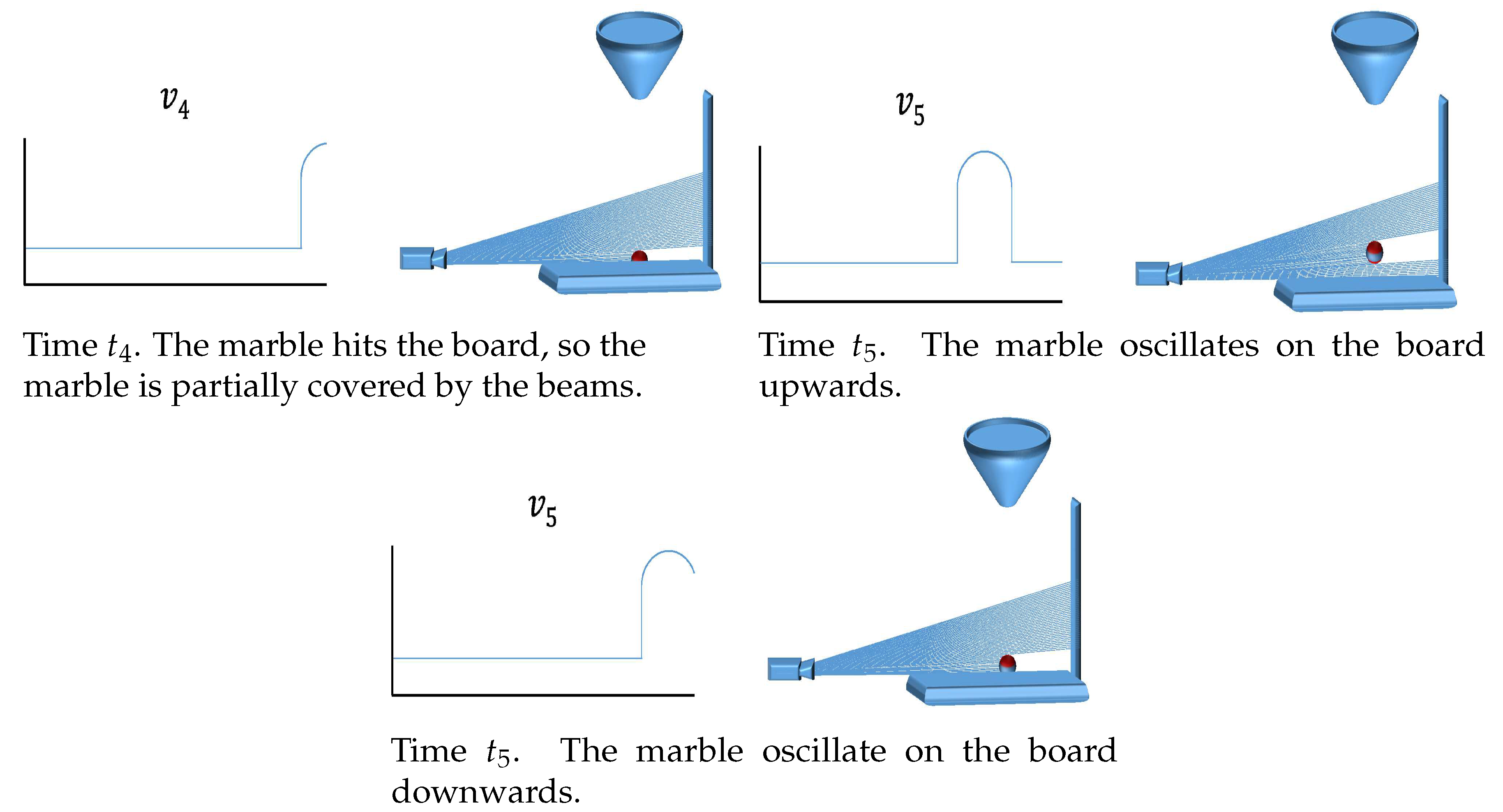
The beam is directed toward this path, so in time , before the ball begins to fall, the depth vector is roughly . Here, the i-th entry of denotes the depth that is sensed by the i-th laser beam. This result stays the same while the ball does not enter the scanned frame of the beams, time , so . When the ball enters the frame of beams, say on , the first beams hit the ball so . In the middle of the fall, time , all the ball enters the frame of the scanner. Then, in time , the ball hits the board, and finally, after hitting the board, time , the ball begins to jump and oscillate. These sets of depth vectors are based on the motion of the ball which is strongly depends on the material of the board.
4.1. Fitting Method
We apply our circle fitting algorithm on the image that corresponds to its vector v, where the x-axis represents the index i which is integer in , and the y-axis represents the value of the i-th index of . The results for some of the vectors over time are shown in Figure 10, where on the right is an illustration of the system state and on the left a graph corresponding to the vector v.
Each of these thousands of measurements required very high precision of circle fitting. We then run our Algorithm 2 to construct a coreset, thereby significantly reducing the number of points in each data set (from hundreds of points to only twenty points), which allows efficient solution using a polynomial system for those thousands of tests.
4.2. Fitting Method Results
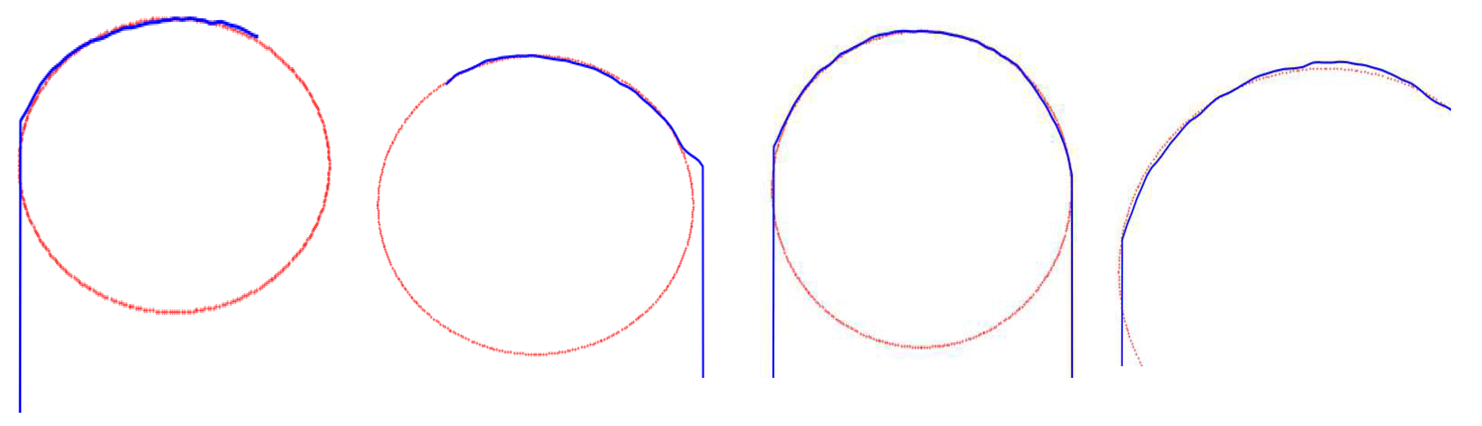
In Figure 11, we show some examples of our fitting results.
5. Conclusions
We suggested a provable and practical algorithm that fits a sphere for a given set of points in the Euclidean d-dimensional space. The algorithm is based on first computing a coreset that is tailored for this problem, and then running the existing inefficient solution on the small coreset. The result is provable for approximation in a provably fast and practical running time for constant d and .
When running the optimal (inefficient) optimal solution on our coreset we indeed obtain running time that is smaller by orders of magnitudes (minutes instead of days) in the price of approximation error. Finally, we run experiments on a real-world physical system that was the main motivation for writing this paper.
Future research directions include generalization to other shapes, proving lower bounds on the size and computation time of the corresponding coreset, and applying the algorithms on more systems.
Author Contributions
Conceptualization, D.E. and D.F.; methodology, D.E. and D.F.; software, D.E.; validation, D.E.; formal analysis, D.E.; investigation, D.E.; resources, D.E.; data curation, D.E.; writing—original draft preparation, D.E.; writing—review and editing, D.F.; supervision, D.F.; All authors have read and agreed to the published version of the manuscript.
Funding
This research received no external funding.
Conflicts of Interest
The authors declare no conflict of interest.
References
- Geiger, A.; Lenz, P.; Urtasun, R. Are we ready for autonomous driving? The kitti vision benchmark suite. In Proceedings of the 2012 IEEE Conference on Computer Vision and Pattern Recognition (CVPR), Providence, RI, USA, 16–21 June 2012; pp. 3354–3361. [Google Scholar]
- Xu, W.; Snider, J.; Wei, J.; Dolan, J.M. Context-aware tracking of moving objects for distance keeping. In Proceedings of the 2015 IEEE on Intelligent Vehicles Symposium (IV), Seoul, South Korea, 28 June–1 July 2015; pp. 1380–1385. [Google Scholar]
- Bonin-Font, F.; Ortiz, A.; Oliver, G. Visual navigation for mobile robots: A survey. J. Intell. Robot. Syst. 2008, 53, 263. [Google Scholar] [CrossRef]
- Oesau, S.; Lafarge, F.; Alliez, P. Planar shape detection and regularization in tandem. In Computer Graphics Forum; Wiley Online Library: Hoboken, NJ, USA, 2016; Volume 35, pp. 203–215. [Google Scholar]
- Xu, K.; Kim, V.G.; Huang, Q.; Kalogerakis, E. Data-driven shape analysis and processing. In Computer Graphics Forum; Wiley Online Library: Hoboken, NJ, USA, 2017; Volume 36, pp. 101–132. [Google Scholar]
- Zhihong, N.; Zhengyu, L.; Xiang, W.; Jian, G. Evaluation of granular particle roundness using digital image processing and computational geometry. Constr. Build. Mater. 2018, 172, 319–329. [Google Scholar] [CrossRef]
- Titsias, M.K. Learning model reparametrizations: Implicit variational inference by fitting mcmc distributions. arXiv 2017, arXiv:1708.01529. [Google Scholar]
- Muggleton, S.; Dai, W.Z.; Sammut, C.; Tamaddoni-Nezhad, A.; Wen, J.; Zhou, Z.H. Meta-Interpretive Learning from noisy images. Mach. Learn. 2018, 107, 1–22. [Google Scholar] [CrossRef] [Green Version]
- Omran, M.; Lassner, C.; Pons-Moll, G.; Gehler, P.; Schiele, B. Neural body fitting: Unifying deep learning and model based human pose and shape estimation. In Proceedings of the 2018 International Conference on 3D Vision (3DV), Verona, Italy, 5–8 September 2018; pp. 484–494. [Google Scholar]
- Estellers, V.; Schmidt, F.; Cremers, D. Robust Fitting of Subdivision Surfaces for Smooth Shape Analysis. In Proceedings of the 2018 International Conference on 3D Vision (3DV), Verona, Italy, 5–8 September 2018; pp. 277–285. [Google Scholar]
- Epstein, D.; Feldman, D. Quadcopter Tracks Quadcopter via Real Time Shape Fitting. IEEE Robot. Autom. Lett. 2018, 3, 544–550. [Google Scholar] [CrossRef]
- acegif.com. Pulsating Ring of Fire. Available online: https://acegif.com/fire-on-gifs (accessed on 10 March 2019).
- VC, H.P. Method and Means for Recognizing Complex Patterns. US Patent 3,069,654, 18 December 1962. [Google Scholar]
- Cuevas, E.; Wario, F.; Osuna-Enciso, V.; Zaldivar, D.; Pérez-Cisneros, M. Fast algorithm for multiple-circle detection on images using learning automata. IET Image Process. 2012, 6, 1124–1135. [Google Scholar] [CrossRef] [Green Version]
- Akinlar, C.; Topal, C. EDCircles: A real-time circle detector with a false detection control. Pattern Recognit. 2013, 46, 725–740. [Google Scholar] [CrossRef]
- Cai, J.; Huang, P.; Chen, L.; Zhang, B. An efficient circle detector not relying on edge detection. Adv. Space Res. 2016, 57, 2359–2375. [Google Scholar] [CrossRef]
- Zhou, X.; Wang, Y.; Zhu, Q.; Miao, Z. Circular object detection in polar coordinates for 2D LIDAR data. In Chinese Conference on Pattern Recognition; Springer: Berlin/Heidelberg, Germany, 2016; pp. 65–78. [Google Scholar]
- Zhang, H.; Wiklund, K.; Andersson, M. A fast and robust circle detection method using isosceles triangles sampling. Pattern Recognit. 2016, 54, 218–228. [Google Scholar] [CrossRef]
- Zhou, B.; He, Y. Fast circle detection using spatial decomposition of Hough transform. Int. J. Pattern Recognit. Artif. Intell. 2017, 31, 1755006. [Google Scholar] [CrossRef]
- Berkaya, S.K.; Gunduz, H.; Ozsen, O.; Akinlar, C.; Gunal, S. On circular traffic sign detection and recognition. Expert Syst. Appl. 2016, 48, 67–75. [Google Scholar] [CrossRef]
- Berkaya, S.K.; Gunal, S.; Akinlar, C. EDTriangles: A high-speed triangle detection algorithm with a false detection control. Pattern Anal. Appl. 2018, 21, 221–231. [Google Scholar] [CrossRef]
- Bae, J.; Cho, H.; Yoo, H. Geometric symmetry using rotational scanning method for circular form detection. In Proceedings of the 2018 IEEE 9th Annual Information Technology, Electronics and Mobile Communication Conference (IEMCON), Vancouver, BC, Canada, 1–3 November 2018; pp. 552–555. [Google Scholar]
- Fischler, M.A.; Bolles, R.C. Random sample consensus: A paradigm for model fitting with applications to image analysis and automated cartography. Commun. ACM 1981, 24, 381–395. [Google Scholar] [CrossRef]
- Camurri, M.; Vezzani, R.; Cucchiara, R. 3D Hough transform for sphere recognition on point clouds. Mach. Vis. Appl. 2014, 25, 1877–1891. [Google Scholar] [CrossRef]
- Tran, T.T.; Cao, V.T.; Laurendeau, D. eSphere: Extracting spheres from unorganized point clouds. Vis. Comput. 2016, 32, 1205–1222. [Google Scholar] [CrossRef]
- Feldman, D. Core-Sets: Updated Survey. In Sampling Techniques for Supervised or Unsupervised Tasks; Springer: Berlin/Heidelberg, Germany, 2020; pp. 23–44. [Google Scholar]
- Jubran, I.; Maalouf, A.; Feldman, D. Introduction to Coresets: Accurate Coresets. arXiv 2019, arXiv:1910.08707. [Google Scholar]
- Har-Peled, S. How to get close to the median shape. In Proceedings of the Twenty-Second Annual Symposium on Computational Geometry, Sedona, AZ, USA, 5–7 June 2006; pp. 402–410. [Google Scholar]
- Agarwal, P.K.; Har-Peled, S.; Varadarajan, K.R. Approximating extent measures of points. J. ACM (JACM) 2004, 51, 606–635. [Google Scholar] [CrossRef]
- Maalouf, A.; Jubran, I.; Feldman, D. Fast and Accurate Least-Mean-Squares Solvers. arXiv 2019, arXiv:1906.04705. [Google Scholar]
- Maple, M. A Division of Waterloo Maple Inc. Waterloo, Ontario. 2016. Available online: https://www.maplesoft.com (accessed on 21 March 2018).
- Inc., W.R. Mathematica, Version 12.0. Available online: https://www.wolfram.com (accessed on 16 April 2019).
- Langberg, M.; Schulman, L.J. Universal ε-approximators for integrals. In Proceedings of the Twenty-First Annual ACM-SIAM Symposium on Discrete Algorithms, Philadelphia, PA, USA, 17–19 January 2010; pp. 598–607. [Google Scholar]
- Feldman, D.; Langberg, M. A unified framework for approximating and clustering data. In Proceedings of the Forty-Third Annual ACM Symposium on Theory of Computing, San Jose, CA, USA, 6–8 June 2011; pp. 569–578. [Google Scholar]
- Braverman, V.; Feldman, D.; Lang, H. New frameworks for offline and streaming coreset constructions. arXiv 2016, arXiv:1612.00889. [Google Scholar]
- Vapnik, V.N.; Chervonenkis, A.Y. On the uniform convergence of relative frequencies of events to their probabilities. In Measures of Complexity; Springer: Berlin/Heidelberg, Germany, 2015; pp. 11–30. [Google Scholar]
- Varadarajan, K.; Xiao, X. A near-linear algorithm for projective clustering integer points. In Proceedings of the Twenty-Third Annual ACM-SIAM Symposium on Discrete Algorithms, SIAM, Kyoto, Japan, 17–19 January 2012; pp. 1329–1342. [Google Scholar]
- Van Rossum, G.; Drake, F.L., Jr. Python Tutorial; Centrum voor Wiskunde en Informatica: Amsterdam, The Netherlands, 1995. [Google Scholar]
- Oliphant, T.E. A Guide to NumPy; Version 1.16.2; Trelgol Publishing: Austin, TX, USA; Available online: https://www.numpy.org (accessed on 26 February 2019).
- Millman, K.J.; Aivazis, M. Python for Scientists and Engineers; Version 1.4.1; Computing in Science and Engineering, University of California: Berkeley, CA, USA; Available online: https://www.scipy.org (accessed on 16 December 2019).
- Team, O.D. OpenCV API Reference 2015. Version 3.4.8. Available online: https://docs.opencv.org/releases (accessed on 12 November 2019).
- Available online: https://github.com/depste01/SphereFitting (accessed on 18 July 2020).
- Kawasaki, M.; Ahn, B.; Kumar, P.; Jang, J.I.; Langdon, T.G. Nano-and Micro-Mechanical Properties of Ultrafine-Grained Materials Processed by Severe Plastic Deformation Techniques. Adv. Eng. Mater. 2017, 19, 1600578. [Google Scholar] [CrossRef] [Green Version]
- Al-Ketan, O.; Rezgui, R.; Rowshan, R.; Du, H.; Fang, N.X.; Abu Al-Rub, R.K. Microarchitected stretching-dominated mechanical metamaterials with minimal surface topologies. Adv. Eng. Mater. 2018, 20, 1800029. [Google Scholar] [CrossRef]
- Gao, L.; Song, J.; Jiao, Z.; Liao, W.; Luan, J.; Surjadi, J.U.; Li, J.; Zhang, H.; Sun, D.; Liu, C.T.; et al. High-Entropy Alloy (HEA)-Coated Nanolattice Structures and Their Mechanical Properties. Adv. Eng. Mater. 2018, 20, 1700625. [Google Scholar] [CrossRef]
Figure 1.
An RGB image that captured a flame of fire [12]. The goal is to approximate the center of the flaming ring.
Figure 1.
An RGB image that captured a flame of fire [12]. The goal is to approximate the center of the flaming ring.

Figure 2.
Coreset’s size vs. approximation error . Experiments on synthetic data points P of different sizes (in colors). The error (y-axis) decreases with coreset’s size (x-axis).
Figure 2.
Coreset’s size vs. approximation error . Experiments on synthetic data points P of different sizes (in colors). The error (y-axis) decreases with coreset’s size (x-axis).

Figure 3.
Running time. Experiment on synthetic data sets for several expected value of error factor (). The measured running time performed for the optimal solution on coreset vs. “RANSAC” algorithm on the full data set and “RANSAC” algorithm on the coreset (“Improved RANSAC”).
Figure 3.
Running time. Experiment on synthetic data sets for several expected value of error factor (). The measured running time performed for the optimal solution on coreset vs. “RANSAC” algorithm on the full data set and “RANSAC” algorithm on the coreset (“Improved RANSAC”).

Figure 4.
The 2D experiments result. The following four graphs show comparison results between coreset sampling by our algorithm with uniform sampling and the same amount of sample data, compared to the RANSAC algorithm (on the full set and on the coreset) that runs at the same time. Each graph displays results for a differently-sized data set.

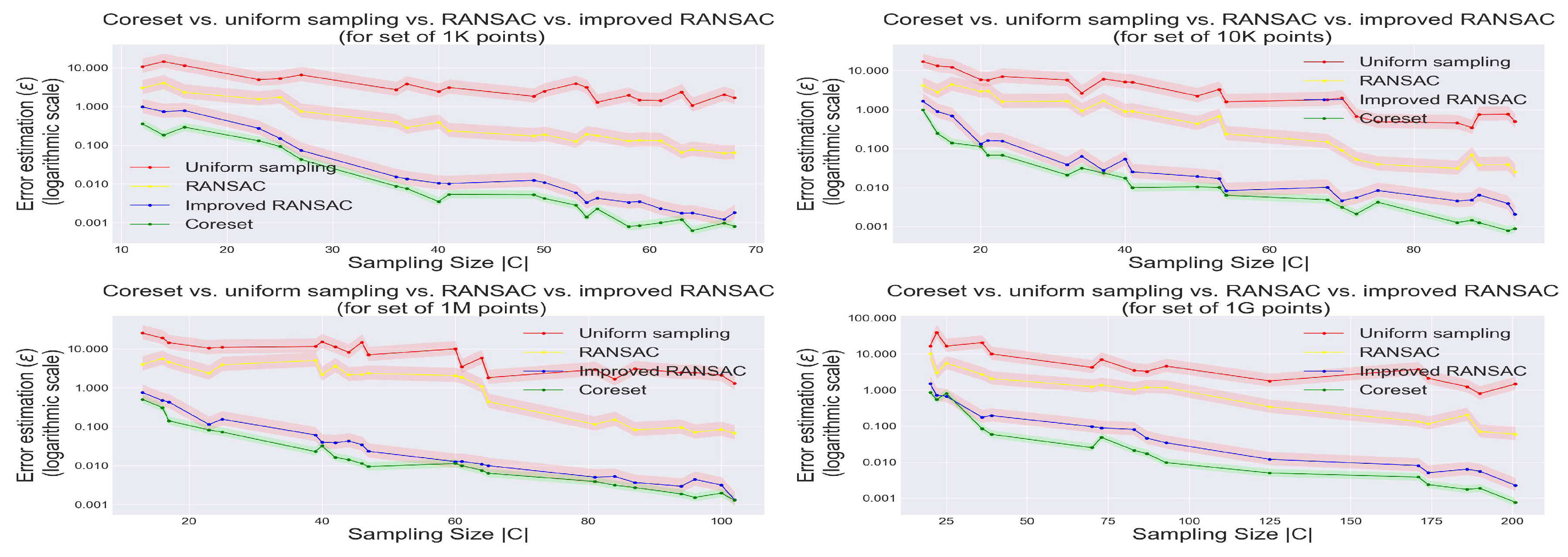
Figure 5.
The 3D experiments result. The following four graphs show comparison results between coreset sampling by our algorithm with uniform sampling and the same amount of sample data, compared to the RANSAC algorithm (on the full set and on the coreset) that runs at the same time. Each graph displays results for a differently-sized data set.

Figure 6.
The 4D experiments result. The following four graphs show comparison results between coreset sampling by our algorithm with uniform sampling with the same amount of sample data, compared to the RANSAC algorithm (on the full set and on the coreset) that runs at the same time. Each graph displays results for a differently-sized data set.

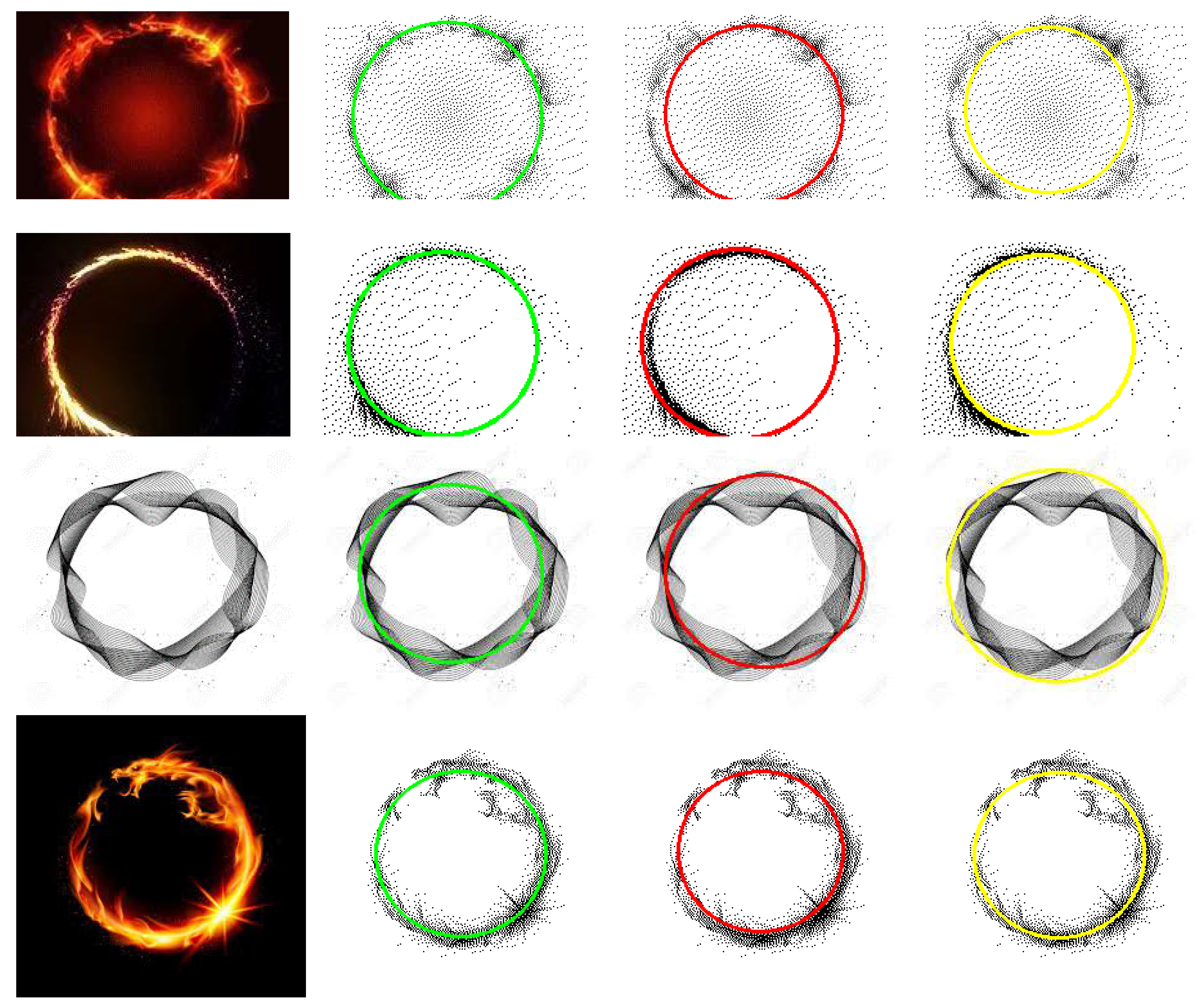
Figure 7.
(Left) An original images. (green) A result for circle detection over real images using our coreset algorithm. (red) A result for circle detection using “Improved RANSAC” algorithm. (yellow) A result for circle detection using “OpenCV”, a widespread open source library heuristic.
Figure 7.
(Left) An original images. (green) A result for circle detection over real images using our coreset algorithm. (red) A result for circle detection using “Improved RANSAC” algorithm. (yellow) A result for circle detection using “OpenCV”, a widespread open source library heuristic.

Figure 8.
Image of the experimental mechanical pressure control system.

Figure 9.
System illustration. (1) Cone for dropping the marble ball (2) marble (3) tested board (material) with pressure sensors below (4) laser device (5) leaser beams (6) white sticker.
Figure 9.
System illustration. (1) Cone for dropping the marble ball (2) marble (3) tested board (material) with pressure sensors below (4) laser device (5) leaser beams (6) white sticker.

Figure 10.
Time step illustration (for ) of the system state (right) and the corresponding depth vector v depending on the laser beam blocking (left).
Figure 10.
Time step illustration (for ) of the system state (right) and the corresponding depth vector v depending on the laser beam blocking (left).


Figure 11.
Circle fitting: The following images show examples for fitting circles (red) to a set of points (blue) with high accuracy as required by the system. Although the samples contain noise and distortions, using our system, we were able to fit an accurate circle to all the samples.
Figure 11.
Circle fitting: The following images show examples for fitting circles (red) to a set of points (blue) with high accuracy as required by the system. Although the samples contain noise and distortions, using our system, we were able to fit an accurate circle to all the samples.

© 2020 by the authors. Licensee MDPI, Basel, Switzerland. This article is an open access article distributed under the terms and conditions of the Creative Commons Attribution (CC BY) license (http://creativecommons.org/licenses/by/4.0/).
Share and Cite
MDPI and ACS Style
Epstein, D.; Feldman, D. Sphere Fitting with Applications to Machine Tracking. Algorithms 2020, 13, 177. https://0-doi-org.brum.beds.ac.uk/10.3390/a13080177
AMA Style
Epstein D, Feldman D. Sphere Fitting with Applications to Machine Tracking. Algorithms. 2020; 13(8):177. https://0-doi-org.brum.beds.ac.uk/10.3390/a13080177
Chicago/Turabian StyleEpstein, Dror, and Dan Feldman. 2020. "Sphere Fitting with Applications to Machine Tracking" Algorithms 13, no. 8: 177. https://0-doi-org.brum.beds.ac.uk/10.3390/a13080177
Note that from the first issue of 2016, this journal uses article numbers instead of page numbers. See further details here.