Scalable Block Preconditioners for Linearized Navier-Stokes Equations at High Reynolds Number


1
School of Mathematics, University of Edinburgh, Edinburgh EH9 3FD, UK
2
Department of Civil Environmental and Architectural Engineering, University of Padua, 35122 Padova, Italy
*
Author to whom correspondence should be addressed.
Algorithms 2020, 13(8), 199; https://0-doi-org.brum.beds.ac.uk/10.3390/a13080199
Submission received: 21 July 2020
/
Revised: 12 August 2020
/
Accepted: 14 August 2020
/
Published: 16 August 2020
Abstract
:We review a number of preconditioners for the advection-diffusion operator and for the Schur complement matrix, which, in turn, constitute the building blocks for Constraint and Triangular Preconditioners to accelerate the iterative solution of the discretized and linearized Navier-Stokes equations. An intensive numerical testing is performed onto the driven cavity problem with low values of the viscosity coefficient. We devise an efficient multigrid preconditioner for the advection-diffusion matrix, which, combined with the commuted BFBt Schur complement approximation, and inserted in a block preconditioner, provides convergence of the Generalized Minimal Residual (GMRES) method in a number of iteration independent of the meshsize for the lowest values of the viscosity parameter. The low-rank acceleration of such preconditioner is also investigated, showing its great potential.
1. Introduction
The task of numerically solving the Navier–Stokes equations is of fundamental importance in many scientific and industrial applications; the strong nonlinearity of the equations and the lack of any theoretical result about existence and regularity of the solutions leaves the scene only to numerical approximations. These have been developed since the beginning of the computing era, but, despite the enormous efforts put into the development of new algorithms, the problem of finding a good solver for most of the practical situations involving the Navier–Stokes equations has always been elusive, particularly when the Reynolds number becomes large. One of the approaches to the numerical solution of the Navier–Stokes equations is given by the Finite Element Method, which, after a linearization of the nonlinear terms, gives rise to a saddle point linear system: this particular system has a structure that appears in many other problems, but in this context it is possible to exploit the underlying continuous formulation to develop efficient preconditioners in the framework of iterative solvers.
In this work, we focus in finding a scalable preconditioner for these saddle point linear systems: many preconditioners have already been developed and tested successfully, for instance in [1,2,3,4,5]; we choose to use the Constraint Preconditioner, already analyzed in all its forms in [6,7,8], and the more popular, in the Fluid Dynamics community, Block Triangular Preconditioner, employed e.g., in [9,10]. We also mention the comprehensive review [11] of preconditioners for saddle point linear systems, and the references therein.
We use the GMRES method and look for a scalable preconditioner, i.e., a preconditioner that allows GMRES to converge in a number of iterations that does not deteriorate as the mesh is refined, in order to obtain an efficient solver. The success of this task lays on finding scalable preconditioners for the block and the Schur complement of the saddle point system. It is well known that a Multigrid technique can be used as a scalable preconditioner for the Poisson problem; the block of our system corresponds to a discrete convection-diffusion operator, which is a variation of a Poisson problem that also involves convective processes. The generalization of Multigrid preconditioners to these kind of situations requires a robust smoother, which can be built using a stationary method involving a pattern that follows the convective flow. This approach has already been tested in [2,12,13].
With regard to the preconditioner for the Schur complement, we will mainly use the preconditioner developed in [9] and improved in [14]. These techniques are based on the assumption that a particular commutator is sufficiently small to neglect it, while they do not exploit the particular underlying structure of the problem, as it happens in the Stokes case.
The problem that we use as test is the well-known 2-dimensional lid-driven cavity, discretized using elements and with values of the viscosity as low as . The main goals that we want to achieve are:
- Develop a smoother that is able to follow the convective flow in the case of the recirculating problem considered; this in turn would allow us to build a scalable Multigrid preconditioner for the block.
- Review and compare a number of Schur complement preconditioners available in the literature.
- Use information on the spectrum of the preconditioned and Schur complement blocks to improve the overall preconditioner and possibly improve scalability in the case of dominating advection.
The rest of the paper is structured as follows: In Section 2, we describe the continuous problem and its weak formulation, while Section 3 is devoted to the development of a stable Mixed Finite Element formulation, the Picard linearization process, and the properties of the saddle point linear systems to be solved at each nonlinear iteration. In Section 4, we describe two block preconditioners for saddle point systems; Section 5 analyzes a number of Multigrid preconditioners for the block and some approximations to the Schur complement matrix. In Section 6, we describe how a low-rank matrix can be used to accelerate the previously described preconditioners. Section 7 provides a thorough numerical testing of the block preconditioners described in the previous sections onto a the challenging lid driven cavity problem, showing the almost perfect scalability of the two most sophisticated variants for the lowest value of the viscosity parameter. Section 8 concludes the paper.
Notation. Throughout the paper, we will write vectors (and vector functions) in boldface. We will use the symbol M to denote a preconditioner which approximates a given coefficient matrix ), while the symbol P will refer to the preconditioner in its inverse form ().
2. Problem Setting and Discretization
The motion of incompressible newtonian fluids is governed by the well known Navier–Stokes equations, a system of partial differential equations that arises from the conservation of mass and momentum. In the general non-stationary case, they take the form
where is the domain in which the motion evolves; is the velocity field; is the pressure field; and are the fluid density and dynamic viscosity; is a forcing term.
The first equation is usually used in a different form: using a unit density, we obtain the following version of the Navier-Stokes equations
where now is the kinematic viscosity, p is the density-scaled pressure field and is a forcing term per unit mass.
The first of the two equations imposes the conservation of momentum; the term takes into account the diffusive processes, while describes the convective processes. The equation imposes the incompressibility of the fluid, i.e., the density is a constant, both in space and time.
For the problem to be well posed, Equations (1) need some initial condition
and boundary conditions, e.g.,
where , and are given functions, and form a partition of the boundary of and is the outward-facing unit normal to .
The first kind of boundary condition is said of Dirichlet type, and will be addressed as the Dirichlet portion of the boundary, while the second kind is said of Neumann type, and will be called the Neumann portion of the boundary.
The Navier–Stokes Equations (1) are nonlinear, due to the term ; moreover, there are no general results about existence, regularity and uniqueness of the solution, in particular in three dimensions. In fact, this is one of the most important open problems in mathematics and one of the Millennium problems.
In the following, we will always consider the stationary Navier–Stokes equations, i.e., Equation (1) without the time derivative of .
2.1. Stokes Equations
Define the Reynolds number as the ratio between inertial and viscous forces, namely , where L is a characteristic length of the domain and U is a representative velocity scale of the fluid. It turns out that, if the Reynolds number is sufficiently small (i.e., if the flow is particularly slow or if the viscosity is high enough), then the Navier–Stokes equations can be simplified: in fact, the term is negligible with respect to the viscous term and the nonlinear Equation (1) become a linear system of equations, known as the stationary Stokes equations:
to which the same previously cited initial and boundary conditions must be applied. In these equations there is no more the presence of convection, but only diffusive processes survive.
The Stokes Equation (2) have the great advantage of being linear, which makes them easier to work with, both analytically and numerically.
2.2. Weak Formulation
The general formulation of Equations (1) and (2), which require as solution a function twice differentiable and a function p continuously differentiable, can be relaxed, allowing for solutions that satisfy weaker requirements. Sometimes, in fact, there does not exist any solution that satisfies the strong form of the equations, while it is possible to find weak solutions.
Before deriving the weak form of the Navier–Stokes equations, let us define the space of square-integrable functions
and the Sobolev Space
i.e., the space of square integrable functions whose derivatives up to order k are still square integrable. Here, represents a weak derivative.
Now, starting from the stationary Navier–Stokes equations, it is possible to obtain the weak formulation multiplying by a test function , where the space V will be definesd later, and integrating over .
In this form, there is still the necessity for the function to be twice differentiable, which is the condition that we want to relax. In order to do so, we exploit Green’s formulas (i.e., integration by parts in multiple dimensions) and rewrite the integral involving as the sum of an integral involving only and a boundary integral. The same can be done for the pressure term. The result is
The same can be done for the second equation, when considering a test function . The result is
Accordingly, an alternative version of the Navier–Stokes equations is: find and such that (3) and (4), together with the proper initial and boundary conditions, hold for every possible choice of and . The couple is then called a weak solution of the Navier–Stokes equations. For this formulation to make sense, all the integrals involved must be well defined: this is achieved by choosing properly the spaces V and Q. The correct choice is to set V equal to the space of functions in such that they satisfy the Dirichlet boundary condition on the Dirichlet portion of the boundary; Q should simply be the space . It can be checked that, in this way, all of the integrals are well defined (see [15]).
3. Finite Element Method
The previously stated weak formulation can be expressed in a more compact form: suppose to solve a Navier–Stokes problem with homogeneous Dirichlet boundary condition on all the boundary. Subsequently, the weak formulation is equivalent to:
Find , such that
where and are bilinear forms, while is a trilinear form, defined as
and
3.1. Galerkin Approximation
Equations (5) are defined on the spaces V and Q, which are subspaces of and of infinite dimension. To develop a numerical scheme that is able to approximate the solution, we need to find an approximate problem defined on spaces of finite dimension. Consider, and , both of finite dimension, then the problem becomes:
The problem with this formulation is that, following the same steps as before, the algebraic system that arises is no more linear, but, due to the trilinear form , it becomes nonlinear. This complicates enormously the method, since solving a nonlinear system of equations involves methods that are far more complicated and computationally costly (e.g., Newton method). The simplest way to solve this problem is to use a fixed-point scheme (known also as Picard iteration) and try to linearize the nonlinear term . This will require an iterative scheme: suppose to start from a given velocity field ; to find the next iterate one could solve Equation (6) where, instead of the nonlinear term, there is the linear term . In this way, the trilinear form that was giving problems becomes simply a bilinear form and can be treated like the other ones. Accordingly, the method can be formalized, as follows
for until convergence. The initial field must be taken divergence free, in order to be consistent with the problem. This can be achieved solving a Stokes problem at the beginning (which assures a divergence-free velocity field) and then using the solution as initial datum for the iteration. This is consistent with setting . This formulation of the Navier–Stokes problem is known as Oseen problem and it is the method that will be used in this work. We refer e.g., to the book [16] for more details.
3.2. Stabilization of the Convection-Diffusion Term
The first terms in the Oseen problem (7) represent a convection-diffusion operator of the form , where the wind is given by the solution of the previous iteration. In the numerical solution of this kind of problems, one important quantity to estimate the stability of the method is the Péclet number, defined as the ratio between convective and diffusive forces, i.e., , where L is a characteristic length and w is the local wind velocity. When discretizing a convection-diffusion problem, this number is used when considering as characteristic length the dimension of the elements. In this way, this parameter is able to tell whether the solution will be stable or not: small values of assure a good solution, while a large leads to instability.
This can be solved using a finer discretization, but when the viscosity is very low, the elements would need to be so small that the computational cost would become enormous. Another option is to use a stabilization technique: instead of solving the unstable problem, one can solve a slight modification of the problem that is stable. This is achieved by adding some artificial diffusion to the problem, which assures that the Péclet number decreases. Of course, the solution will be slightly different from the real one, but it will be at least stable. If the stabilization is done correctly, then the solution will not be affected too much.
There exist various methods of stabilization; in this work, the simplest one will be used, called streamline diffusion (SD), which adds diffusion only in the direction of the wind. Other approaches include the Streamline upwind Petrov–Galerkin (SUPG), the Algebraic subgrid scale (ASGS) stabilized Finite Elements, and the Galerking Least-Square (GLS) methods, but their theory and implementation are far more complicated, and they are beyond the scope of this paper (see [15] for more details). The SD method introduces another bilinear form in the formulation of the Navier–Stokes equations, defined as
where is defined as follows: call the mesh Péclet number, with h the local dimension of the element. Subsequently, if , is set to zero, i.e., no stabilization is performed on those elements where is sufficiently small. Instead, where
This choice of the stabilization parameter is taken from [2].
This stabilization technique will be useful when solving the Navier–Stokes equation with low values of viscosity.
3.3. Choice of the Finite Element Spaces
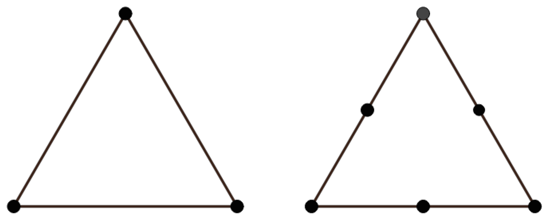
The choice of Finite Element spaces and must satisfy the well-known inf-sup (or LBB) condition [2]. The lowest order pair uses functions for the space and functions for . This type of choice is sometimes referred to as Taylor-Hood approximation and it will be the one used in this work. Figure 1 shows the two kind of elements used for the spaces and .
3.4. Algebraic Formulation
Let us now denote with a basis of , and with a basis for . The unknown functions and in (7) can be written as a linear combination of these basis functions, as
At each iteration of the Picard method, a linear system has to be solved, which takes the following form
where and contain the unknowns and , i.e., the values of velocity and pressure of the approximated solution on the nodes of the grid. Linear systems with this particular block structure are usually called saddle point systems.
In the following, represents the element-wise product of two vectors and , while represents the Euclidian scalar product. The matrix A is the discrete vector Laplacian
the matrix B is called the divergence matrix and is defined as
The matrix N is the discrete vector convection matrix, which depends on the current estimate of the velocity and has the following definition
The block of (8) will be referred to as matrix .
Notation. In the sequel, we will denote as the size of the block in (8), while will indicate the number of rows of B.
We will now define some other matrices that will be useful later: the velocity-mass matrix and the (pressure-)mass matrix as
They are both square, symmetric, and positive definite. From the point of view of operators, the mass matrix corresponds to a discrete identity operator.
3.5. Properties of Saddle Point Matrices
Theorem 1.
Consider a problem where (no Neumann boundary conditions), discretized using a stable approximation on a shape-regular quasi-uniform subdivision of . Subsequently, the Schur complement is spectrally equivalent to the pressure mass matrix Q:
where β is the inf-sup constant.
Proof.
See [2]. □
This theorem has an important consequence: regardless of how much we refine the mesh, the matrix will always have its eigenvalues on a very narrow interval. Moreover, it will always be positive semi-definite (as is in the kernel of the Schur complement, so it is not positive definite, being singular) and, because Q is positive definite, also the Schur complement will always be positive semi-definite. Let us define h as the maximum diameter (diam) of all elements K in the discretization, whereas diam. Then, matrix has a condition number that can be bounded independently of the size h of the discretization. This property does not hold for matrix A, whose condition number that grows indefinitely as h goes to 0. This fact plays a crucial role in the numerical solution of the Stokes and Navier–Stokes equations.
A similar result also holds if the Neumann boundary is non-empty; in this case, the upper bound is 2. Again, for all further details, see [2].
4. Block Preconditioners for the Navier-Stokes Discretized Systems
The following results are in the line of those e.g., of [17,18,19], in which symmetric saddle point matrices are considered.
4.1. Block Triangular Preconditioner
We will now analyze the Block Triangular Preconditioner (BTP) applied to the discretized Navier–Stokes equations. Let us define H the Navier–Stokes coefficient matrix and M the preconditioner:
with and scalable preconditioners for F and for the negative Schur complement , respectively. From now on, scalability will denote the property of a given preconditioner to produce roughly the same number of iterations as the mesh is refined. In other words, the eigenvalues of the preconditioned matrices will be uniformly bounded in h.
To analyze the eigenvalues of the preconditioned matrix , we assume that there exist LU factorizations of and and define
Subsequently, the eigenvalue problem is equivalent to
Defining and exploiting the blocks, we obtain
where is similar to the preconditioned block .
Matrices R and N satisfies:
where is the exact (minus) Schur complement related to the matrix
and hence represents this Schur complement, preconditioned by the spectrally equivalent matrix . Observing that the matrix on the right in (11) is involutory we rewrite (11) as
which finally reads
Writing now and , (13) rewrites as
We have shown that the BTP-preconditioned matrix is similar to a matrix that can be written as one with all eigenvalues at one plus another one whose norm is bounded by the norms of and .
4.2. Inexact Constraint Preconditioner
Using the previous definition, we can define the Inexact Constraint Preconditioner ICP as
The adjective inexact arises when the exact Schur complement is replaced by an approximation, , as it is in this case. This implies that the block of is no longer zero, as it is in the Constraint Preconditioner. As before, pre- and post- multiplying by and yields an eigenvalue problem equivalent to :
Matrix on the right in (15) is easily decomposed, recalling that , as
It turns out that is similar to the matrix
in view of (14). We have shown that the ICP-preconditioned matrix is similar to a matrix that can be written as the identity matrix of order plus a matrix whose norm is bounded by the norms of and .
The results developed for ICP and BTP preconditioned matrices show that unit eigenvalues are perturbed by the presence of error matrices and whose norms, in the case of scalable preconditioners for the blocks, swill be small and independent of the mesh discretization parameter h. This is a pleasant property, which, in many cases, is responsible of fast convergence of the GMRES method. However, it is well known [20] that a clustering of the eigenvalues around the unit value is not sufficient to guarantee fast convergence of the GMRES method due to the possible ill-conditioning of the matrix of the eigenvectors. Analyses based on the field of values of the preconditioned matrix have been carried out for simplified preconditioners in order to overcome this theoretical problem. See, e.g., [21,22].
4.3. Relaxation
In case the spectral regions of the preconditioned block and the preconditioned Schur complement are not perfectly overlapped, the influence of a relaxation parameter has been investigated in [7], where, however, the two block matrices are both SPD. In short, the relaxation parameter acts on the block of the Inexact Constraint Preconditioner, as
with to be chosen so that the smallest of the two previously mentioned spectral regions is included in the other one.
5. Preconditioners for the Blocks
Any block preconditioner for a saddle-point linear system, like the one that we considered, can only yield scalable results if the preconditioners used to approximate the block and the Schur complement are scalable. Therefore, the main task is to find such suitable preconditioners for the two blocks involved.
5.1. Block Preconditioner
It is well known that Multigrid methods allow for obtaining scalable results for convection-diffusion problems. Our block indeed represents a discretized convection-diffusion operator and, therefore, we expect to obtain scalable results while using a suitable Multigrid scheme. An accurate analysis of the scalability provided by Multigrid can be found, for instance, in [23,24].
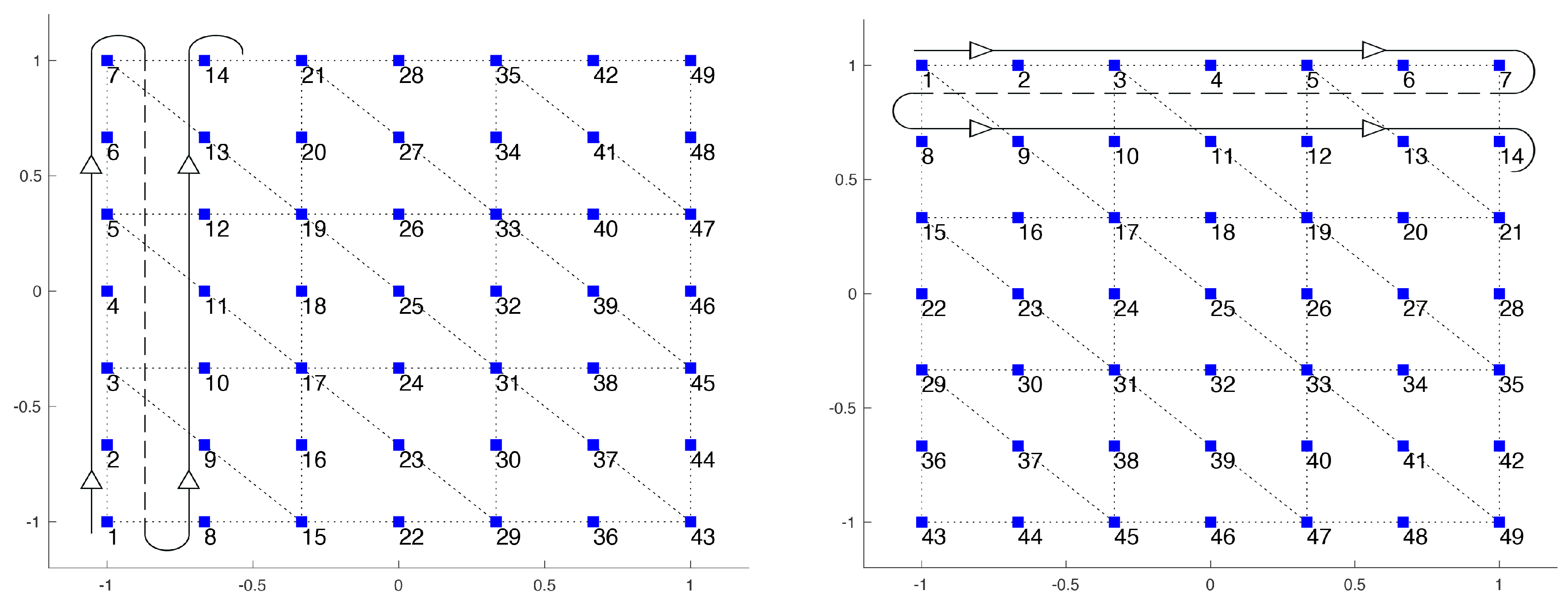
The application of a Multigrid preconditioner is particularly easy in the case of diffusion-dominated problems, since even the very simple damped Jacobi smoother is able to produce optimal results. However, in the case of convection-dominated problems, the choice of the smoother is fundamental for obtaining satisfactory results. In these situations, it is necessary to use a more sophisticated smoother, like the Gauss–Seidel method, coupled with an adequate choice of the pattern used to apply it; this pattern should try to follow the convective flow as much as possible. In the case of complicated recirculating flows, it is not possible to generate a pattern that is able to do this and so different strategies must be employed. In [2], the suggestion is to use multiple iterations of the Gauss-Seidel smoother, each one performed following a simple pattern. In particular, if the flow is recirculating and therefore has components both negative and positive in directions x and y, then there should be four patterns and they should sweep through the domain in both directions, going back and forth. Hence, one pattern will evolve in the x direction, from the left to the right, another one from right to left. The same holds for the y direction, yielding a total of four different smoothing patterns. An alternative using only one pattern in every direction is possible: this approach will be cheaper, but a single iteration will be less accurate. This option has been used, for instance, in [13] when dealing with convection-diffusion problems.
One thing to remember is that, when multiple patterns are used for every smoothing iteration, they should be applied in opposite order in the pre- and post-smoothing phases. If in the pre-smoothing step, we apply first pattern A and then pattern B, then in the post smoothing phase we should apply first pattern B and then A.
The drawback of using multiple patterns is that some parts of the flow, which only have component of the velocity in one direction, do not need smoothing in the other direction. Thus, a lot of time is lost smoothing in directions that are not necessary. This is not a problem for convergence, since this excessive smoothing does not worsen the solution, but it is a problem for the computational time. Moreover, this approach does not exploit the separability of the block: indeed, the convection-diffusion operator consists of a block-diagonal matrix, with two identical blocks, one for direction x and one for y. This structure of the matrix can be exploited to obtain a more efficient implementation: indeed, when applying the preconditioner to a vector r, we can split this vector into and and apply to each of these components just the preconditioner for one of the diagonal blocks of matrix F. In this way, the dimensions of the matrices used are halved and, more importantly, we can choose to perform the smoothing only in the direction that we are considering. This means that when we apply the preconditioner to , we use Gauss–Seidel with a pattern that only evolves in the x direction. We do not expect more accurate solutions with this method, since applying extra smoothing does not create such a problem, but we expect to reduce the computational time required.
Two approaches are possible when applying one of the patterns in the smoothing phase. We can divide the pattern in groups and apply the smoother to all the nodes of every group simultaneously; for instance, if the pattern to be applied evolves in the x direction, then each group would be one of the vertical lines of nodes. In this way, the smoother updates all of the values for these nodes at once, which is the best approach possible. However, in this way, the linear system to be solved inside Gauss–Seidel is block triangular and not triangular. Alternatively, we can apply the smoother to every node individually; in this way, the system to be solved is triangular, but along every line, some nodes are updated before and some others later. We used the second approach, as the results were very similar, but the computational time was lower.
In the numerical experiments, we tested four different approaches, which are summarized in the following:
- Jacobi, which identifies the Multigrid scheme using the simple damped Jacobi smoother.
- simple-GS, which indicates the use of Gauss-Seidel with lexicographic ordering.
- 2dir-GS, which identifies the Gauss-Seidel smoother applied with two patterns, one for every direction.
- split-GS, which indicates the new approach that exploits the structure of the block.
The patterns that are used in the last two approaches are shown in Figure 2 for a small grid.
Besides the smoother, there are other aspects of the Multigrid preconditioner that must be treated with care when dealing with convection-dominated problems. Stabilization needs to be taken into account: when passing from one grid to the next, the matrix to be used in the following grid must be the exact matrix, with the accurate stabilization; the Galerkin coarse grid operator should be avoided, because the coarser grids need stabilization, while the fine ones may not need it. In our experiments, we used streamline diffusion stabilization.
The restriction and prolongation operators can be taken to be the natural ones, i.e., the ones obtained exploiting the values of the basis functions over the nodes of the discretizations. Finally, we need to choose the cycle to be used: a V-cycle would be cheaper, but it may need more iterations to obtain the same accuracy. We chose to use a W-cycle instead, which requires more computational effort, but more closely clusters the eigenvalues around one. However, as we shall see in the next section, the Multigrid method is also used by the Schur complement preconditioner. In that case, we made a different choice of cycle.
5.2. Schur Complement Preconditioner
Let us now focus on finding a scalable preconditioner for the Schur complement. In the case of diffusion-dominated problems, then the mass matrix or even a diagonal approximation of it can produce scalable results. Indeed, for the Stokes problem, which represents the limit case where convection is not present, the pressure mass matrix is spectrally equivalent to the Schur complement.
The difficult challenge is to find a scalable preconditioner in the case of convection-dominated problems. The first approaches used the mass matrix that was scaled by the viscosity. This choice, although very simple, does not yield scalable results in general. Therefore, more complicated preconditioners are necessary. We now summarize some of these alternatives.
5.2.1. PCD Preconditioner
The Pressure convection-diffusion (PCD) approach can be intuitively justified when considering the operator that the Schur complement represents: matrix is the discrete counterpart of the continuous operator , where represents the local wind (given by the solution of the previous iteration in the case of the Oseen problem). We can think of a preconditioner for the Schur complement as an approximation of the discrete version of the inverse of this operator: then, calling the convection-diffusion operator built in the pressure space and the corresponding Laplacian, we can assume that matrix is an approximation for . However, in the case of diffusion-dominated problems, and tend to coincide, yielding the identity matrix as preconditioner. Premultiplying by , the pressure mass matrix, we can assure that in this extreme case the preconditioner goes back to the known optimal alternative.
This preconditioner was proposed and derived formally in [4] and studied thoroughly in [25]. It provides a significant improvement with respect to the scaled mass matrix, keeping the computational cost low: matrices and are indeed smaller than F and L, making this preconditioner particularly efficient. However, the rate of convergence seems to suffer when gets close to zero, even for simple problems. Moreover, matrix is not used in the original problem and, thus, needs to be built at every Picard iteration; the proper boundary conditions to apply to it are not straightforward to choose and they do not necessarily coincide with the conditions applied to the original problem. An analysis of this issue can be found in [14].
5.2.2. BFBt Preconditioner
A different preconditioner can be derived in a more algebraic way: in [9], it is proved that, under the assumption that , the exact inverse of the Schur complement is given by matrix
Hence, we can take as a preconditioner for the Schur complement, even if the assumption does not hold in general. Further analysis showed that an improvement can be obtained when considering the scaled version
which, in the case of continuous pressure elements, simplifies to
where is the velocity mass matrix, or an approximation of it. This preconditioner is clearly more expensive than the PCD, since it involves two applications of and a product with matrix F instead of . However, most of the matrices used are already available and the additional boundary conditions to apply to represent a less critical problem. Dependence on the mesh size and on the viscosity is observed, especially for complicated flows.
5.2.3. Commuted BFBt Preconditioner
An improvement to the BFBt preconditioner was proposed in [14], where they analyzed the continuous counterpart of matrix (18) and suggested to commute some of the operators involved, yielding the preconditioner
where L is the diffusive part of matrix F. This alternative is even more expensive than the previous one, since matrix L is larger than . On the positive side, all of the matrices are already available and there are no new boundary conditions to apply. Moreover, the inversion of matrix L can be performed with the same Multigrid technique used to precondition matrix F.
This last alternative is the one that has showed the best results in term of scalability, even if some dependence on the mesh size can still be observed for very low viscosities and complicated flows. It is also worth pointing out that, in the case of diffusion-dominated problems, this approach behaves decisively worse than PCD.
5.2.4. Augmented Lagrangian Approach
We briefly sketch a completely different approach from the ones previously presented: suppose modifying the block of the original saddle-point linear system, so that the matrix becomes
where is a parameter and W is positive definite. The solution is not changed, but it is now possible to simplify the Schur complement and find a very efficient preconditioner. As shown in [1], if W is taken to be the pressure mass matrix, an optimal choice for is simply . However, this great efficiency in the Schur complement preconditioner is balanced by the need for a much more complicated Multigrid scheme for the new block. In [3], this approach was generalized to the three dimensional case and it was also pointed out that the highly specialized Multigrid scheme used depends on the choice of the discretization and it may not be possible to use this method with every such choice.
In our numerical experiments, we chose to use preconditioner (19), since it is the one with the best chance of providing scalable results for a recirculating flow and since it does not involve matrices to be computed separately. Moreover, it exploits the same Multigrid that we used for the block, which means that any improvement that we make there also has an impact on the Schur complement.
Some comments must be made regarding the Multigrid used to invert matrix L. We used the same strategy used for matrix F, with the following differences: since no convection is present, we found out that using the V cycle is sufficient to provide good results; we performed a larger number of cycles, since, in this case, we would like to obtain the exact inverse of L and not just a preconditioner. We maintained the approach of splitting matrix L, since this allows for saving computational time.
6. Low-Rank Update of the Block Preconditioner
6.1. Left Preconditioning
Consider the generic linear system . Following [26], given an initial preconditioner and a tall, full-rank, matrix V, the Broyden-tuning preconditioner is defined as
with the property that
Hence, the preconditioned matrix has the eigenvalue 1 with multiplicity (at least) p. The best choice of the columns of V is represented by the eigenvectors of corresponding to the outlier eigenvalues. Let us assume then that the columns of V are approximate eigenvectors of the initially preconditioned matrix:
with and is small enough. The eigenvalues are decreasingly ordered with respect to the function .
Neglecting matrix E we can simplify the low-rank preconditioner as
with small matrix to be built once and for all before starting of the iteration process.
6.2. Right Preconditioning
The Broyden preconditioner inherits the tuning condition (21) as a reformulation of the secant equation, which only holds for left preconditioning. However, it can be easily reformulated to handle the case of right preconditioning, as follows
satisfying now
The unpleasant presence of in this expression can be eliminated reasoning as before and assuming that now and, therefore, , so that we can define an approximate, but more effective right preconditioner as
Differently from the left preconditioning the preprocessing stage now requires p applications of the preconditioner to form matrix W.
6.3. Avoiding Complex Eigenpairs
One possible obstacle to this approach is the fact that both V and are likely to be complex. This is solved by constructing a real invariant subspace of the same size, as described in Algorithm 1.
| Algorithm 1 Constructing a real invariant subspace for the preconditioned matrix. |
|
By construction matrices Z and (which is no longer diagonal) approximately satisfy and the low-rank left preconditioner is defined consequently as
Analogously the right preconditioner is modified with in place of .
6.4. Application of the Low-Rank Approach to the Blocks
Starting from our block preconditioners we can apply the low-rank correction either to the (1,1) block only or also to the Schur complement preconditioner. We consider then two cases, both in the framework of the left preconditioning:
- Let be the (inverse of the) multigrid preconditioner for the block and consider the left preconditioner (22). To compute the relevant eigenpairs we run the nonrestarted Arnoldi method with as the subspace size for the preconditioned matrix . Then we selected all the p eigenvalues satisfying and the corresponding eigenvectors as columns of to form the updated preconditioner for the block as
- In addition to the previous, define the (inverse of the) Schur complement preconditioner to be used in (22) and run the nonrestarted Arnoldi method for the preconditioned matrix , where is the Schur complement of the block preconditioner defined asAgain, we consider all of the eigenvalues satisfying and form the updated Schur complement preconditioner as
7. Numerical Results
In this Section, we will show the results of the numerical experiments performed; the spectral properties of the matrices will be used to predict the behavior of a certain technique and we will then compare the predictions with the actual results. Some plots will be used to compare the spectra of different preconditioners and show convergence profiles of GMRES.
7.1. Model Problem
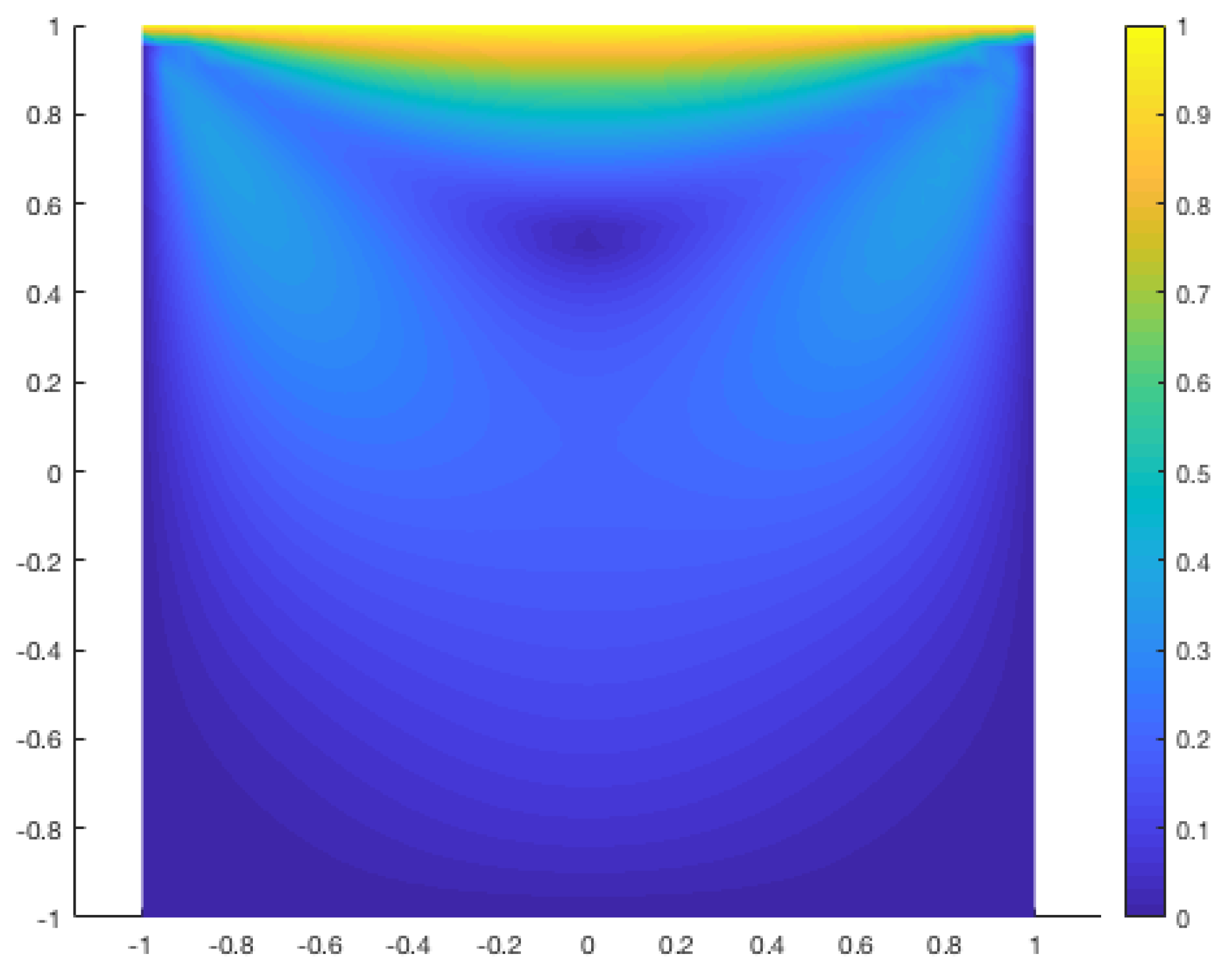
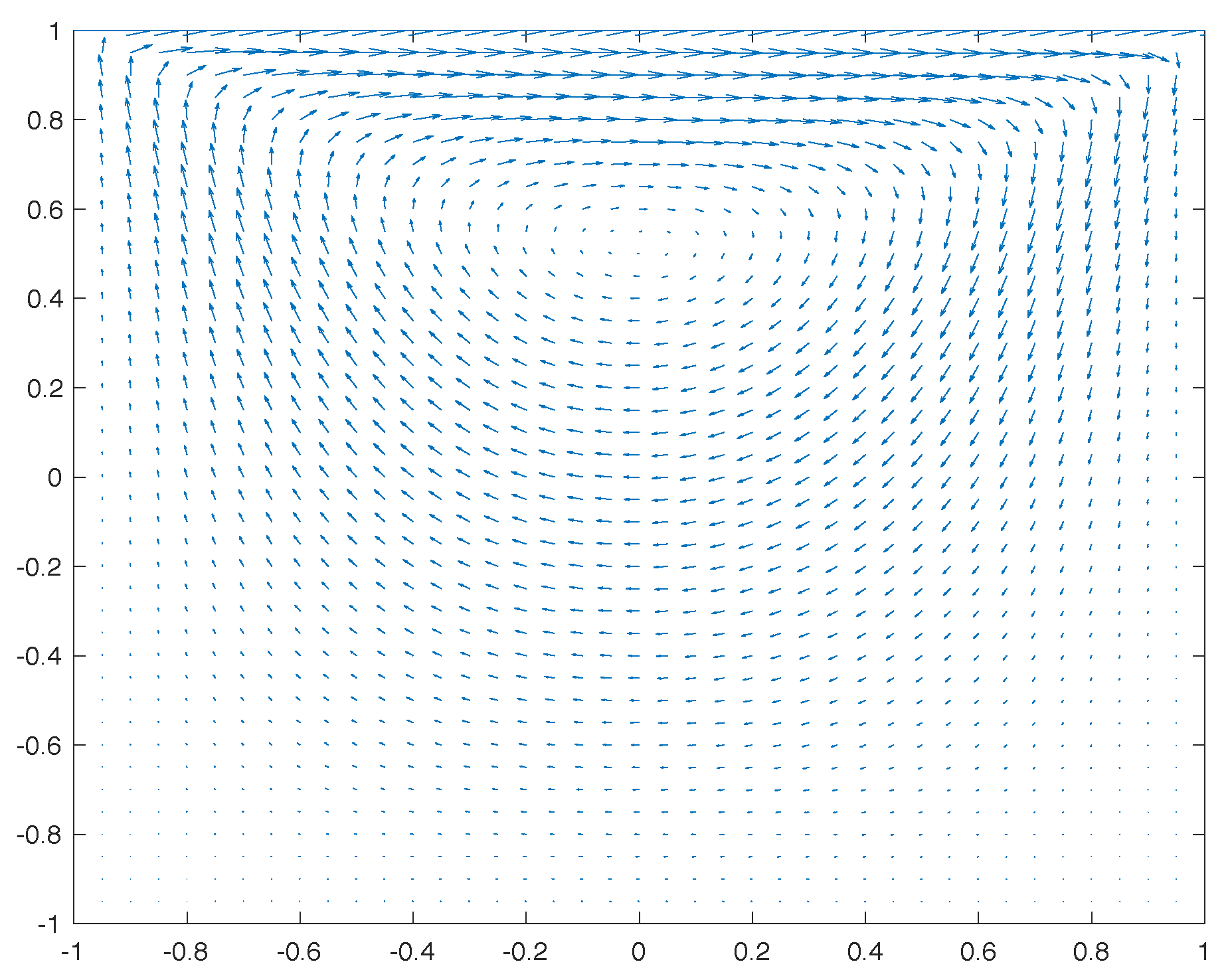
The model problem that is used in this work is the well-known lid-driven cavity problem; a thorough description of this problem can be found in [27]. The source term is set to zero, the viscosity is set to 1 for the Stokes equations, while it varies between and for the Navier–Stokes equations. The domain corresponds to the two-dimensional square . The equations, together with the boundary conditions, are
The problem evolves inside a square domain; on the two lateral sides and on the bottom side, there is a no-slip condition (i.e., the velocity is zero), while on the top side there is an horizontal velocity imposed. There is no normal velocity on any portion of the boundary, thus the flow is enclosed (no fluid can enter or exit the domain).
7.2. Problem Description
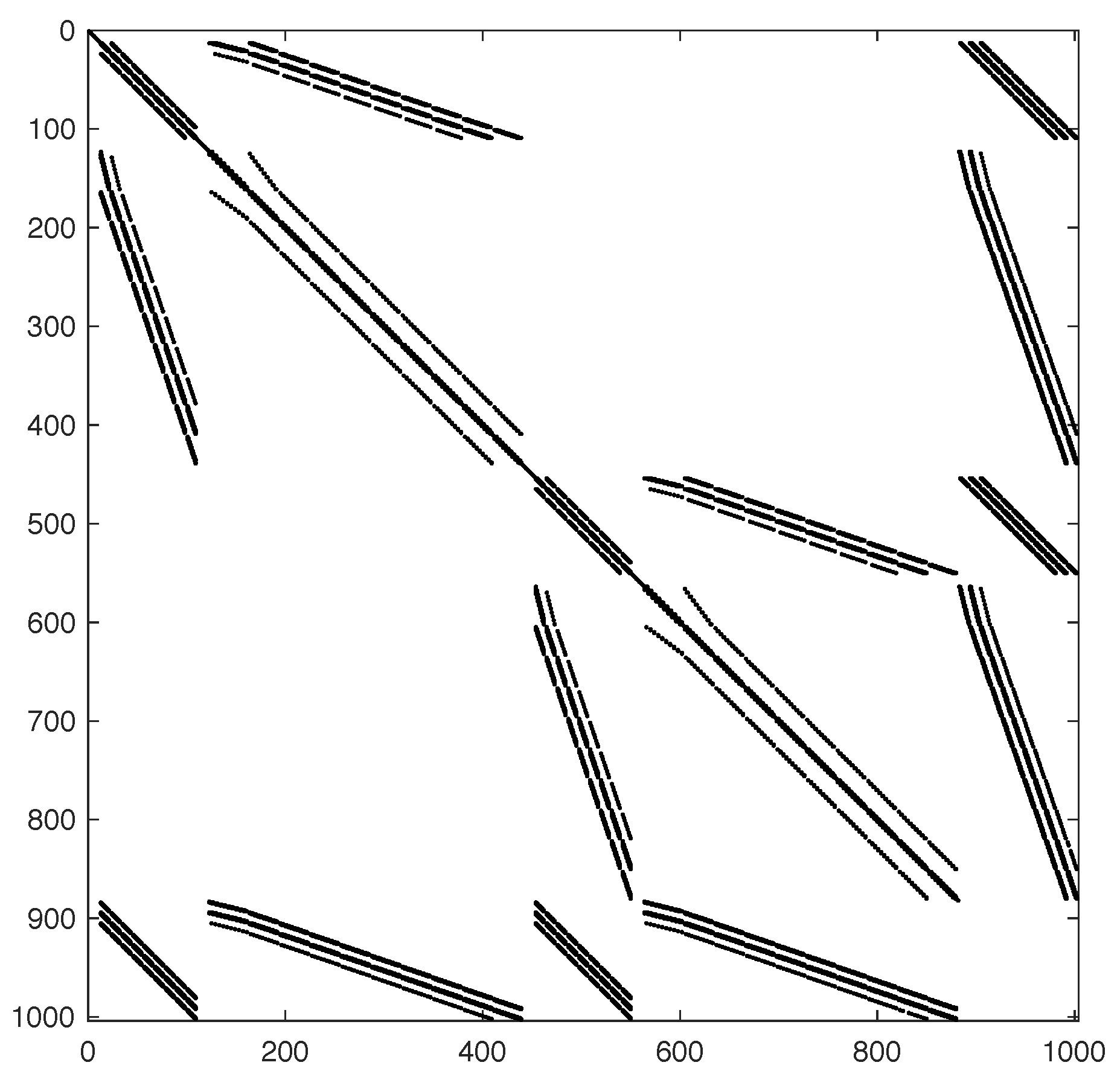
The matrices used for the numerical tests are generated using values of n from 10 to 320. In particular, Table 1 illustrates all of the matrices used, showing their dimension and number of nonzero entries, while Figure 5 shows the sparsity pattern the matrix M10.
The number of nonzero entries per row vary between 14 and 18 and the density increases as n grows. The smaller matrices M10 and M20 will only be used in the layer of the Multigrid preconditioner, while the other will be actually used as matrices for the saddle point system.
Concerning the Navier–Stokes equations, the matrices used are obtained after five iterations of a Picard scheme, which ensures that the nonlinear phenomena are well represented. The value of the viscosity is set to 1 for the Stokes problem. For the Navier–Stokes equations, it will assume the values , , , and . Lowering the viscosity, the system will become more asymmetric, which is expected to worsen the properties of the preconditioner.
The numerical results will regard the Navier–Stokes equations, for which we will be analyzing both the spectral properties and number of iterations required for the GMRES to converge. It is worth pointing out that the scalability of the results would not change using another Krylov subspace solver, e.g., BICGSTAB, since the preconditioner is derived based on the properties of the underlying problem, and not considering the specific solver used. The notation will be the following: and represent the maximum and minimum eigenvalues in modulus of the preconditioned block; and represent the maximum and minimum eigenvalues in modulus of the preconditioned Schur complement (obviously, the zero eigenvalue of the Schur complement is not considered, since it is always present).
7.3. Some Details on Implementation
All of the results have been obtained using codes written in Matlab on a laptop with equipped with an Intel processor i5-8350U quad core with 16GB RAM. The finite elements have been implemented using a four-point Gaussian quadrature scheme. The eigenvalue estimates are obtained using the Arnoldi method. The solver used is left-preconditioned GMRES with a tolerance of and without restart. Using the right-preconditioned version instead would not change the obtained scalability results. See the brief discussion in Section 7.8. All of the times reported are in seconds. The † symbol in the Tables will denote no convergence within 400 iterations.
7.4. Multigrid and BFBt
We now report the results that were obtained using the various Multigrid schemes and the BFBt preconditioner. These results are not scalable, due to the poor smoothers and the non-scalable implementation of the BFBt preconditioner. Hence, we will only show the results in terms of the iteration count. We will also show the eigenvalue distribution, which helps to understand the quality of the Multigrid smoother. The Multigrid parameters will be shown as , where m is the number of cycles used, V or W represent the type of cycle used, and and indicate the number of pre and post smoothing steps. The coarsest level for Multigrid in these tests is the matrix M10.
7.4.1. Jacobi/BFBt
The first combination involves a damped Jacobi smoother; the Multigrid used is , while the BFBt preconditioner is implemented using an incomplete factorization.
Table 2 reports the spectral properties of the preconditioned matrices.
The eigenvalues of the preconditioned block show a slight dependence on the mesh size ( is decreasing, is increasing), even for the highest viscosity, which represents a problem that is similar to the Stokes one. The smallest eigenvalue does not seem to be affected by the value of the viscosity, while the biggest one grows substantially with the viscosity, getting in the worst case to a value larger than 5. The fact that the spectral properties deteriorate as the viscosity grows is perfectly in line with the fact that this Multigrid preconditioner was built for a symmetric problem, while lowering the viscosity makes the problem increasingly asymmetric. For an even lower viscosity (), the eigenvalues become negative, leading to a complete failure of the preconditioner.
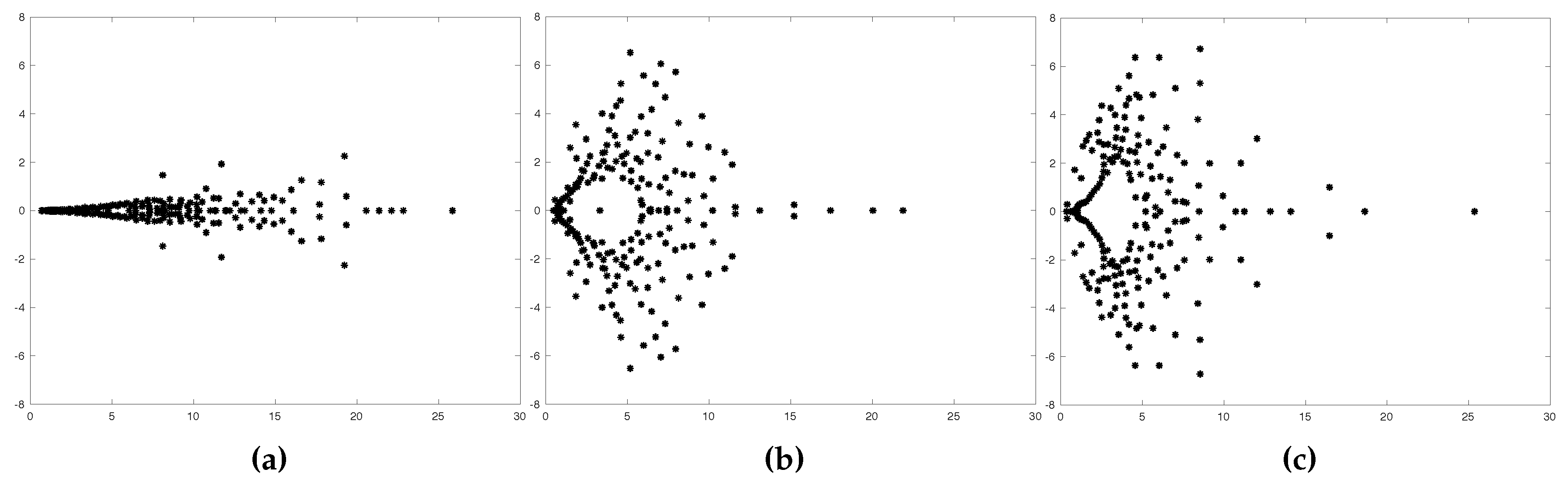
The situation is not better for the Schur complement preconditioner: even in this case, the spectral interval widens as the mesh is refined. Moreover, the eigenvalues are less clustered around 1, as the spectral radius is always above 20.
Figure 6 illustrates the spectrum of the preconditioned Schur complement for various values of the viscosity. Every dot represents an eigenvalue in the complex plane (only the first 100 eigenvalues found by Arnoldi are represented). These spectra do not depend on the Multigrid scheme used, so they would be the same as even using a different Multigrid. It is clear that, as the viscosity gets lower, the system becomes more asymmetric and, consequently, the imaginary part of the eigenvalues increases.
Table 3 shows the results obtained with Jacobi and BFB: even with very high viscosity, the preconditioner is not scalable; for low viscosity instead, it fails completely.
7.4.2. Simple GS/BFBt
Using the simple Gauss–Seidel method as smoother is expected to improve the results, but it still should not be scalable, since the smoothing is performed following the original numbering of the nodes and not following the convective flow. The Multigrid is again . Table 4 shows the spectral properties in this case.
There is a great improvement in the eigenvalue bounds of the preconditioned block for the highest viscosity: indeed, the spectral interval is extremely narrow and focused around 1. However, this nice property disappears for the lowest viscosity, even leading to negative eigenvalues for the matrix M80. That is exactly what we expected: for high viscosities, the convection phenomena are not relevant; hence, there is not much difference between smoothers that follow or not the flow. Instead, for low viscosities, the convection process must be taken into account to produce a suitable smoother.
Table 5 shows the results in this case: they are still not scalable and again for low viscosities convergence is not achieved.
7.4.3. Two-Direction GS/BFBt
The next combination uses a Gauss–Seidel smoother applied using two patterns that try to follow the convective flow. We also employed a W cycle, which means that the Multigrid used is now . Table 6 shows the spectral properties.
The results are promising, at least for the Multigrid preconditioner: the smallest eigenvalue is very close to 1 and it does not suffer from refinement of the mesh or reduction in the viscosity. The spectral radius is slightly above 1 and again does not deteriorate too much changing the properties of the problem: there is a little growth when the viscosity is reduced and there is a decrease when the mesh is refined (this can be explained noticing that the convective phenomena are better represented when the matrix is larger, therefore improving the efficiency of this Multigrid scheme that is based on these phenomena).
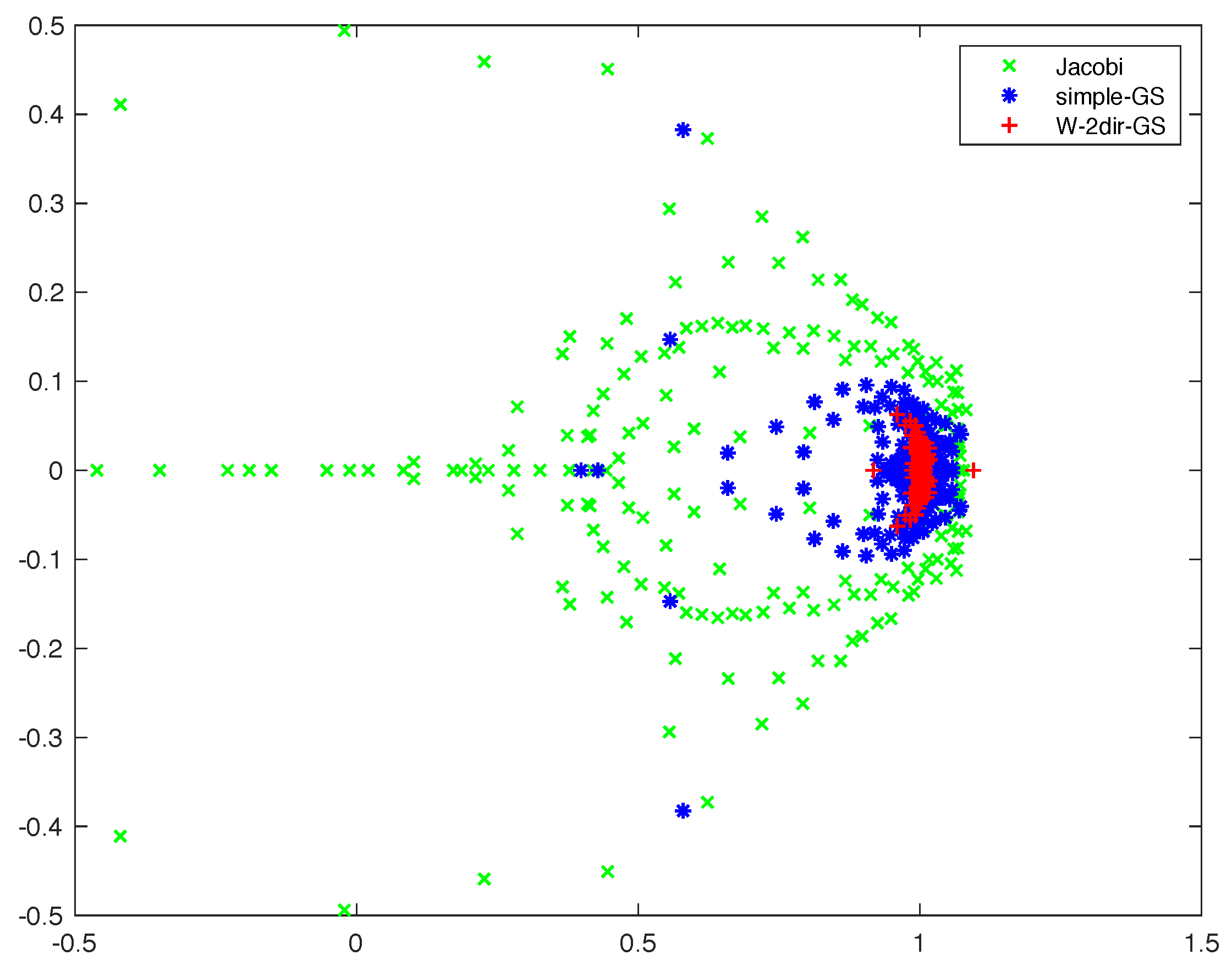
Figure 7 shows the spectrum of the preconditioned block while using the three previous smoothers. It is clearly visible how only the last choice is able to cluster the eigenvalues around one. Table 7 displays the results with this combination: they are again not scalable, but the behavior for the lowest viscosity is improved, thanks to the more efficient smoother.
In Table 7, we also show the effect of the relaxation parameter , as proposed in [7], and briefly described at the end of Section 4, with the aim of improving the condition number of the preconditioned matrices. Setting provides a slight decrease in the number of iterations, and this is due to the spectra of the preconditioned blocks, which partially overlap. Because of these (not completely satisfactory) preliminary results, the relaxation parameter will not be employed in the next results.
7.5. Multigrid and BFBt-c
To obtain scalable results, we used the BFBt-c preconditioner, which was also implemented using a Multigrid scheme. In the following tables, we also show the true residual tres of the solution computed by GMRES (). This datum is useful to understand the quality of the preconditioner: indeed, using left preconditioning, the exit test of GMRES is performed with the residual of the preconditioned system, which may differ substantially from the residual of the actual system. Moreover, we also show the computational time, which includes the time to build the preconditioner, apply it’s and solve the linear system with GMRES.
The coarsest level for Multigrid in these tests is the matrix M20.
7.5.1. Jacobi/BFBt-c
The first test involves the Jacobi smoother; the Multigrid in this case is for the block and for the BFBt-c preconditioner.
The results are shown in Table 8: we can see that, for high viscosities, the results are scalable, but the preconditioner fails when using low viscosities, providing erratic iteration numbers.
7.5.2. Simple GS/BFBt-c
We then used the simple Gauss-Seidel smoother with the BFBt-c preconditioner, with the same parameters as before. The results, shown in Table 9, show an improved behavior, with good results also in the case of . However, for the lowest viscosity, the non-scalability remains.
7.6. Handling the Low Viscosity Case. Two-Direction GS/BFBt-c
The next test is performed using the 2dir GS smoother and the BFBt-c preconditioner. The Multigrid for the block is now .
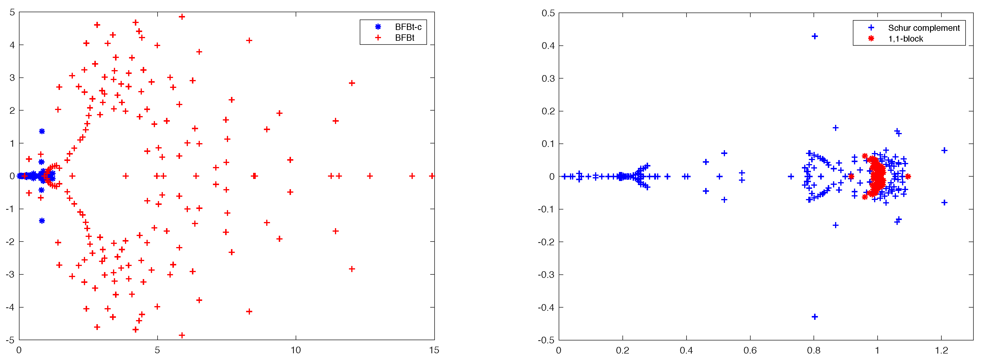
In Figure 8 (left), we compare the spectrum of BFBt and BFBt-c, while, in Figure 8 (right), we show the spectrum of the block and the one of the BFBt-c preconditioned Schur complement. The plot reveals the clear superiority of the BFBt-c preconditioner, which provides a better clustering of the eigenvalues.
To better follow the circulant flow with so high Reynolds number, we choose to select as the coarsest mesh M20 instead of M10. As a first consequence, the cost per iteration is expected to increase, mainly for the smallest problems.
Table 10 shows the results while using this combination. The preconditioners are scalable for all viscosities, confirming the promising impression that we got from the spectral information. However, the true residual of the final solution is a couple of orders of magnitude larger than the original tolerance of GMRES.
To try saving some of the added computational time, we employed strategy split-GS, which is supposed to be cheaper than 2dir-GS. We show the results in Table 11: when compared with Table 10, these results indeed show a lower computational time, revealing, as expected, that split-GS is a cheap variant of 2dir-GS. However, it also introduces some instabilities that prevent the reduction of the true residual in some cases.
If we compare Table 8, Table 9, Table 10 and Table 11, we can see that, for high viscosities, the results are scalable using any method. In this situation, the most efficient approach in terms of computational time is the one that involves the Jacobi smoother, since the convection is not sufficiently strong to justify the use of a complicated flow-following technique. However, when it comes to low viscosities, the Gauss–Seidel smoother with proper ordering is the only strategy that manages to produce scalable results.
We also report the results while using a Block Triangular Preconditioner, as shown in Table 12. The higher number of iterations needed is balanced by the reduced cost per iteration, producing a final computational time that is better than in the previous case. However, the true residual gets even higher in some cases.
The low-rank update, whose effects will be described next, will mitigate this effect.
7.7. Handling the Low Viscosity Case. Preconditioner Update by Low-Rank Matrices
We have obtained a scalable preconditioner for all viscosities considered using, as the coarsest level, the matrix M20 instead of M10, which implies a high computational cost at each application of the Multigrid. This choice is necessary, since using matrix M10 produces the spectral distribution that is shown in Table 13, where the Multigrid is completely unable to properly precondition the block.
The situation that is depicted by Table 13 is a promising situation that suggests the use of the low-rank update: the number of outlier for the preconditioned F block is relatively small and does not roughly change with the meshsize. On the contrary, updating the preconditioner for the Schur complement block does not seem to be advisable, as the eigenvalues of this block are not much far away from 1.
The results where the split-GS based preconditioner is used in combination with the low-rank update for the block, as described in Section 6, are reported in Table 14. We employed 50 non-restarted Arnoldi iterations to assess the corresponding eigenvectors (as they are well separated, Arnoldi convergence reveals very fast). The preprocessing time that is related to this task is reported in the Table as prep. The results using the Constraint Preconditioner and the BTP are summarized in Table 14.
The results show that this approach yields similar results as in the previous Tables, with two exceptions: first, the fact that we selected M10 as the coarsest mesh provided a notable reduction of the CPU time per iterations. Second, the true norm of the residual is much lower, showing a closer relation between the residual provided by the GMRES method and the true residual, and suggesting the better conditioning of the preconditioner. Moreover, the preprocessing time to assess dominant eigenvectors is around of the overall CPU time. Scalability with respect to h is almost perfect, the number of iterations, on the average, being slightly increased with respect to starting from M20 mesh with no update.
7.8. Comparisons with Right-Preconditioned GMRES
As anticipated, the scalability results obtained so far with the left-preconditioned GMRES would also be confirmed by the right-preconditioned GMRES implementation. It is well-known that, in this last case, the exit test is on the true residual (instead of the preconditioned residual). However this advantage is in some instances purely theoretical as the exact residual may be much different from the computed residual due to ill-conditioning of the systems matrices. We report in Table 15 the results for and both BTP and ICP approaches while using the right-preconditioned GMRES, to be compared with the last columns in Table 11 and Table 12 and with Table 14. The results confirm the optimal scalability of the proposed preconditioner.
8. Conclusions
The algebraic solution of the discretized and linearized Navier Stokes equations, in case of high Reynolds number, is still a challenging numerical linear algebra problem. Our contribution is to give an overview of the main multigrid approaches to precondition the advection-diffusion block and to approximate the Schur complement matrix. We have also proposed some variants that can improve efficiency and scalability of the block preconditioner in the case of low viscosity value. The use of such sophisticated multigrid variants leads to solving the finest Navier–Stokes discretized system with almost one-million unknowns and 17 million nonzeros in a few minutes, even for the smallest () value of the viscosity. We have also shown that the use of low-rank updates may constitute a viable improvement of a given block preconditioner when the number of the eigenvalues of the preconditioned block, which are far away from 1 (outliers) is small and roughly independent of h.
Author Contributions
Writing—original draft preparation, F.Z. and L.B.; writing—review and editing, F.Z. and L.B. All authors have read and agreed to the published version of the manuscript.
Funding
This research has been funded by the project granted by the Fondazione Cassa di Risparmio di Padova e Rovigo (CARIPARO): Matrix-Free Preconditioners for Large-Scale Convex Constrained Optimization Problems (PRECOOP).
Acknowledgments
We are indebted to M. Nozza for providing the initial version of the multigrid code and for fruitful discussions.
Conflicts of Interest
The authors declare no conflict of interest.
References
- Benzi, M.; Olshanskii, M. An augmented Lagrangian-based approach to the Oseen problem. SIAM J. Sci. Comput. 2006, 28, 2095–2113. [Google Scholar] [CrossRef]
- Elman, H.; Sylvester, D.; Wathen, A. Finite Elements and Fast Iterative Solvers, 2nd ed.; Oxford University Press: Oxford, UK, 2014. [Google Scholar]
- Farrell, P.; Mitchell, L.; Wechsung, F. An augmented Lagrangian preconditioner for the 3D stationary incompressible Navier-Stokes equations at high Reynolds number. SIAM J. Sci. Comput. 2019, 41, A3073–A3096. [Google Scholar] [CrossRef] [Green Version]
- Kay, D.; Loghin, D.; Wathen, A. A Preconditioner for the Steady-State Navier-Stokes Equations. SIAM J. Sci. Comput. 2002, 24, 237–256. [Google Scholar] [CrossRef]
- Silvester, D.; Elman, H.; Kay, D.; Wathen, A. Efficient preconditioning of the linearized Navier-Stokes equations for incompressible flow. J. Comput. Appl. Math. 2001, 128, 261–279. [Google Scholar] [CrossRef] [Green Version]
- Bergamaschi, L.; Ferronato, M.; Gambolati, G. Mixed Constraint Preconditioners for the solution to FE coupled consolidation equations. J. Comput. Phys. 2008, 227, 9885–9897. [Google Scholar] [CrossRef]
- Bergamaschi, L.; Martínez, A. RMCP: Relaxed Mixed Constraint Preconditioners for Saddle Point Linear Systems Arising in Geomechanics. Comp. Methods Appl. Mech. Engrg. 2012, 221–222, 54–62. [Google Scholar] [CrossRef] [Green Version]
- Keller, C.; Gould, N.; Wathen, A. Constraint Preconditioning for Indefinite Linear Systems. SIAM J. Matrix Anal. Appl. 2000, 21, 1300–1317. [Google Scholar] [CrossRef] [Green Version]
- Elman, H. Preconditioning For The Steady-State Navier-Stokes Equations With Low Viscosity. SIAM J. Sci. Comput. 2001, 20, 1299–1316. [Google Scholar] [CrossRef] [Green Version]
- Elman, H. Preconditioners for saddle point problems arising in computational fluid dynamics. Appl. Numer. Math. 2002, 43, 75–89. [Google Scholar] [CrossRef] [Green Version]
- Benzi, M.; Golub, G.H.; Liesen, J. Numerical solution of saddle point problems. Acta Numer. 2005, 14, 1–137. [Google Scholar] [CrossRef] [Green Version]
- Olshanskii, M.; Reusken, A. Convergence analysis of a multigrid method for a convection-dominated model problem. SIAM J. Numer. Anal. 2004, 42, 1261–1291. [Google Scholar] [CrossRef] [Green Version]
- Ramage, A. A multigrid preconditioner for stabilised discretisations of advection-diffusion problems. J. Comput. Appl. Math. 1999, 110, 187–203. [Google Scholar] [CrossRef] [Green Version]
- Olshanskii, M.; Vassilevski, Y. Pressure Schur Complement Preconditioners for the Discrete Oseen Problem. SIAM J. Sci. Comput. 2007, 29, 2686–2704. [Google Scholar] [CrossRef]
- Quarteroni, A. Numerical Models for Differential Problems, 2nd ed.; Springer: Milan, Italy, 2012. [Google Scholar]
- Elman, H.C.; Silvester, D.J.; Wathen, A.J. Finite Elements and Fast Iterative Solvers: With Applications in Incompressible Fluid Dynamics; Numerical Mathematics and Scientific Computation, Oxford University Press: New York, NY, USA, 2014. [Google Scholar]
- Benzi, M.; Simoncini, V. On the eigenvalues of a class of saddle point matrices. Numer. Math. 2006, 103, 173–196. [Google Scholar] [CrossRef] [Green Version]
- Simoncini, V. Block triangular preconditioners for symmetric saddle-point problems. Appl. Numer. Math. 2004, 49, 63–80. [Google Scholar] [CrossRef]
- Bergamaschi, L. On Eigenvalue distribution of constraint-preconditioned symmetric saddle point matrices. Numer. Linear Algebra Appl. 2012, 19, 754–772. [Google Scholar] [CrossRef] [Green Version]
- Greenbaum, A.; Pták, V.; Strakoš, Z. Any Nonincreasing Convergence Curve is Possible for GMRES. SIAM J. Matrix Anal. Appl. 1996, 17, 465–469. [Google Scholar] [CrossRef] [Green Version]
- Klawonn, A.; Starke, G. Block triangular preconditioners for nonsymmetric saddle point problems: Field-of-values analysis. Numer. Math. 1999, 81, 577–594. [Google Scholar] [CrossRef]
- Benzi, M.; Olshanskii, M.A. Field-of-Values Convergence Analysis of Augmented Lagrangian Preconditioners for the Linearized Navier–Stokes Problem. SIAM J. Numer. Anal. 2011, 49, 770–788. [Google Scholar] [CrossRef] [Green Version]
- Trottenberg, U.; Oosterlee, C.; Schuller, A. Multigrid; Academic Press: London, UK, 2001. [Google Scholar]
- Wesseling, P. An Introduction to Multigrid Methods; John Wiley and Sons: Chichester, UK, 1992. [Google Scholar]
- Loghin, D.; Wathen, A.J. Schur complement preconditioners for the Navier-Stokes equations. Int. J. Numer. Methods Fluids 2002, 40, 403–412. [Google Scholar] [CrossRef]
- Bergamaschi, L. A Survey of Low-rank Updates of Preconditioners for Sequences of Symmetric Linear Systems. Algorithms 2020, 13, 100. [Google Scholar] [CrossRef] [Green Version]
- Kuhlmann, H.; Romanò, F. The Lid-Driven Cavity. Comput. Methods Appl. Sci. 2019, 50, 233–309. [Google Scholar]
Figure 1.
Linear and quadratic triangular elements, used in the Taylor-Hood approximation.

Figure 2.
Ordering of the nodes for the smoothing.

Figure 3.
Velocity magnitude for the Stokes problem.

Figure 4.
Velocity direction for the Stokes problem.

Figure 5.
Sparsity pattern of matrix M10.

Figure 6.
Spectra of the BFBt-preconditioned Schur complement for different values of viscosity. (a) ; (b) ; (c) .
Figure 6.
Spectra of the BFBt-preconditioned Schur complement for different values of viscosity. (a) ; (b) ; (c) .

Figure 7.
Spectra of various Multigrid schemes for the matrix M40 and .

Figure 8.
On the left, the spectra of the preconditioned Schur complement for BFBt and BFBt-c preconditioners. On the right the spectra of the preconditioned block and the Schur complement using BFBT-c. Plots referring to matrix M40 and .
Figure 8.
On the left, the spectra of the preconditioned Schur complement for BFBt and BFBt-c preconditioners. On the right the spectra of the preconditioned block and the Schur complement using BFBT-c. Plots referring to matrix M40 and .


Table 1.
Properties of the matrices.
| Matrix | Dimension | NNZ |
|---|---|---|
| M10 | 1003 | 14,280 |
| M20 | 3803 | 62,008 |
| M40 | 14,803 | 258,268 |
| M80 | 58,403 | 1,054,076 |
| M160 | 232,003 | 4,258,388 |
| M320 | 924,803 | 17,118,310 |
Table 2.
Spectral properties of the preconditioned matrices using Jacobi and BFBt.
| Matrix | Viscosity | ||||
|---|---|---|---|---|---|
| M40 | 0.1 | 0.4256 | 1.261 | 0.6926 | 25.86 |
| 0.01 | 0.4251 | 1.905 | 0.4746 | 21.87 | |
| M80 | 0.1 | 0.3555 | 1.442 | 0.2107 | 26.62 |
| 0.01 | 0.3588 | 2.911 | 0.1494 | 25.92 | |
| M160 | 0.1 | 0.3371 | 1.700 | 0.0557 | 39.41 |
| 0.01 | 0.3383 | 5.013 | 0.1744 | 28.97 |
Table 3.
Results using Jacobi and BFBt. The † symbol means no convergence within 400 iterations.
| Matrix | |||
|---|---|---|---|
| M40 | 67 | 110 | † |
| M80 | 97 | 195 | † |
| M160 | 141 | 336 | † |
Table 4.
Spectral properties of the preconditioned matrices while using sGS and BFBt.
| Matrix | Viscosity | ||||
|---|---|---|---|---|---|
| M40 | 0.1 | 1.0000 | 1.002 | 0.6966 | 25.44 |
| 0.01 | 0.9784 | 1.006 | 0.4527 | 21.83 | |
| 0.005 | 0.6591 | 1.422 | 0.2522 | 25.15 | |
| M80 | 0.1 | 1.0000 | 1.003 | 0.2159 | 26.47 |
| 0.01 | 0.9984 | 1.015 | 0.1290 | 25.82 | |
| 0.005 | <0 | 19.35 | 0.0349 | 27.95 |
Table 5.
Results using sGS and BFBt. The † symbol means no convergence within 400 iterations.
| Matrix | |||
|---|---|---|---|
| M40 | 64 | 107 | † |
| M80 | 87 | 183 | † |
| M160 | 135 | 334 | † |
Table 6.
Spectral properties of the preconditioned matrices using 2dir GS and BFBt.
| Matrix | Viscosity | ||||
|---|---|---|---|---|---|
| M40 | 0.1 | 0.9907 | 1.022 | 0.6973 | 25.46 |
| 0.01 | 0.9912 | 1.133 | 0.4899 | 21.84 | |
| 0.005 | 0.9153 | 1.291 | 0.1962 | 25.20 | |
| M80 | 0.1 | 0.9907 | 1.027 | 0.2159 | 26.55 |
| 0.01 | 0.9889 | 1.032 | 0.1242 | 25.83 | |
| 0.005 | 0.9619 | 1.130 | 0.0350 | 25.25 | |
| M160 | 0.1 | 0.9908 | 1.036 | 0.0554 | 27.20 |
| 0.01 | 0.9874 | 1.036 | 0.0315 | 26.68 | |
| 0.005 | 0.9859 | 1.050 | 0.0283 | 26.46 |
Table 7.
NS-W2dGS-BFBt results for various values of the relaxation parameter. The † symbol means no convergence within 400 iterations.
Table 7.
NS-W2dGS-BFBt results for various values of the relaxation parameter. The † symbol means no convergence within 400 iterations.
| M40 | M80 | M160 | |||||||
|---|---|---|---|---|---|---|---|---|---|
| 0.1 | 0.01 | 0.005 | 0.1 | 0.01 | 0.005 | 0.1 | 0.01 | 0.005 | |
| 1 | 64 | 107 | 118 | 88 | 181 | 253 | 136 | 330 | † |
| 0.5 | 62 | 104 | 115 | 86 | 177 | 249 | 135 | 328 | † |
| 0.25 | 61 | 102 | 111 | 85 | 174 | 246 | 133 | 325 | † |
| 0.1 | 59 | 100 | 112 | 82 | 171 | 242 | 129 | 321 | † |
| 0.05 | 59 | 113 | 134 | 81 | 174 | 265 | 128 | 319 | † |
Table 8.
Results using Jacobi and BFBt-c.
| Matrix | |||||||||
|---|---|---|---|---|---|---|---|---|---|
| iter | time | tres | iter | time | tres | iter | time | tres | |
| M20 | 45 | 1.76 | 2.40 × 10⁻³ | 59 | 2.29 | 3.33 × 10⁻³ | 99 | 3.83 | 3.56 × 10⁻² |
| M40 | 49 | 3.49 | 3.30 × 10⁻³ | 65 | 4.53 | 3.90 × 10⁻³ | 215 | 15.77 | 4.06 × 10⁻² |
| M80 | 53 | 8.76 | 2.20 × 10⁻³ | 69 | 11.46 | 3.50 × 10⁻³ | 232 | 39.45 | 1.22 × 10⁻² |
| M160 | 55 | 38.46 | 1.11 × 10⁻³ | 71 | 50.04 | 2.10 × 10⁻³ | 113 | 82.38 | 4.60 × 10⁻³ |
| M320 | 55 | 162.95 | 4.69 × 10⁻⁴ | 73 | 215.95 | 1.10 × 10⁻³ | 121 | 420.06 | 1.50 × 10⁻³ |
Table 9.
Results using sGS and BFBt-c.
| Matrix | |||||||||
|---|---|---|---|---|---|---|---|---|---|
| iter | time | tres | iter | time | tres | iter | time | tres | |
| M20 | 43 | 1.70 | 2.00 × 10⁻⁴ | 56 | 2.21 | 8.85 × 10⁻⁴ | 55 | 2.18 | 1.78 × 10⁻² |
| M40 | 47 | 3.49 | 1.32 × 10⁻⁴ | 60 | 4.47 | 6.75 × 10⁻⁴ | 78 | 5.75 | 1.25 × 10⁻² |
| M80 | 50 | 8.87 | 3.43 × 10⁻⁵ | 63 | 11.20 | 1.66 × 10⁻⁴ | 91 | 16.23 | 1.60 × 10⁻³ |
| M160 | 52 | 39.91 | 3.49 × 10⁻⁵ | 62 | 47.67 | 1.32 × 10⁻⁵ | 103 | 81.14 | 5.58 × 10⁻⁴ |
| M320 | 53 | 171.20 | 9.57 × 10⁻⁵ | 65 | 211.05 | 3.71 × 10⁻⁵ | 111 | 370.35 | 2.74 × 10⁻⁴ |
Table 10.
Results using 2dir-GS and BFBt-c.
| Matrix | ||||||||||||
|---|---|---|---|---|---|---|---|---|---|---|---|---|
| iter | time | tres | iter | time | tres | iter | time | tres | iter | time | tres | |
| M40 | 46 | 14.08 | 1.8 × 10⁻⁵ | 52 | 21.14 | 4.6 × 10⁻⁵ | 60 | 18.53 | 3.0 × 10⁻⁴ | 80 | 24.49 | 1.5 × 10⁻² |
| M80 | 49 | 33.99 | 1.5 × 10⁻⁵ | 55 | 49.64 | 2.3 × 10⁻⁵ | 65 | 42.35 | 7.6 × 10⁻⁵ | 85 | 56.16 | 6.9 × 10⁻³ |
| M160 | 52 | 125.01 | 8.9 × 10⁻⁶ | 53 | 127.17 | 1.4 × 10⁻⁵ | 66 | 158.49 | 2.1 × 10⁻⁵ | 93 | 224.67 | 9.3 × 10⁻⁴ |
| M320 | 52 | 589.25 | 1.1 × 10⁻⁶ | 52 | 614.96 | 1.1 × 10⁻⁵ | 66 | 651.42 | 1.3 × 10⁻⁵ | 99 | 1128.95 | 1.4 × 10⁻⁴ |
Table 11.
Results using ICP with split-GS and M20 as the coarsest mesh.
| Matrix | ||||||||||||
|---|---|---|---|---|---|---|---|---|---|---|---|---|
| iter | time | tres | iter | time | tres | iter | time | tres | iter | time | tres | |
| M40 | 47 | 13.13 | 1.6 × 10⁻⁴ | 53 | 14.76 | 1.5 × 10⁻⁴ | 62 | 16.97 | 4.7 × 10⁻⁴ | 82 | 22.31 | 1.5 × 10⁻² |
| M80 | 50 | 27.43 | 1.7 × 10⁻⁴ | 52 | 28.10 | 8.2 × 10⁻⁵ | 64 | 35.47 | 5.2 × 10⁻⁴ | 89 | 49.34 | 5.5 × 10⁻³ |
| M160 | 52 | 75.46 | 3.2 × 10⁻⁴ | 56 | 81.91 | 5.7 × 10⁻⁶ | 67 | 98.77 | 1.4 × 10⁻⁴ | 94 | 140.11 | 6.4 × 10⁻³ |
| M320 | 55 | 312.79 | 3.3 × 10⁻⁴ | 58 | 332.21 | 1.5 × 10⁻⁵ | 67 | 384.49 | 1.2 × 10⁻⁴ | 99 | 697.55 | 1.9 × 10⁻³ |
Table 12.
Results using BTP with split-GS and M20 as the coarsest mesh.
| Matrix | ||||||||||||
|---|---|---|---|---|---|---|---|---|---|---|---|---|
| iter | time | tres | iter | time | tres | iter | time | tres | iter | time | tres | |
| M40 | 52 | 11.66 | 1.20 × 10⁻³ | 55 | 11.93 | 1.62 × 10⁻⁴ | 71 | 15.37 | 4.43 × 10⁻⁴ | 94 | 20.29 | 2.10 × 10⁻³ |
| M80 | 55 | 24.46 | 5.20 × 10⁻³ | 57 | 22.98 | 2.31 × 10⁻⁴ | 72 | 28.83 | 6.64 × 10⁻⁵ | 102 | 41.56 | 1.50 × 10⁻³ |
| M160 | 58 | 63.11 | 1.55 × 10⁻³ | 59 | 63.81 | 4.29 × 10⁻⁴ | 72 | 78.87 | 1.57 × 10⁻⁴ | 106 | 118.64 | 1.60 × 10⁻³ |
| M320 | 62 | 281.67 | 5.29 × 10⁻² | 59 | 273.62 | 1.20 × 10⁻³ | 67 | 301.17 | 3.90 × 10⁻⁴ | 108 | 493.86 | 1.66 × 10⁻⁴ |
Table 13.
Spectral properties of the preconditioned matrices with viscosity using the coarsest matrix M10.
Table 13.
Spectral properties of the preconditioned matrices with viscosity using the coarsest matrix M10.
| Matrix | # Outliers | # Outliers | ||
|---|---|---|---|---|
| in the (1,1) Block | in the Schur Complement | |||
| M40 | 11 | 22.8 | 4 | 2.9 |
| M80 | 10 | 511.9 | 7 | 3.7 |
| M160 | 10 | 10 | 3.4 |
Table 14.
Results using split-GS and low-rank update for with ICP (left) and BTP (right). The coarsest mesh is M10.
Table 14.
Results using split-GS and low-rank update for with ICP (left) and BTP (right). The coarsest mesh is M10.
| Inexact Constraint Preconditioner | Block Triangular Preconditioner | |||||||||
|---|---|---|---|---|---|---|---|---|---|---|
| Matrix | Iter | Time | tres | Iter | Time | tres | ||||
| prep | GMRES | Total | prep | GMRES | Total | |||||
| M20 | 115 | 0.51 | 4.85 | 5.36 | 6.60 × 10⁻³ | 93 | 0.55 | 5.23 | 5.78 | 9.80 × 10⁻³ |
| M40 | 86 | 1.38 | 9.29 | 10.67 | 2.40 × 10⁻³ | 106 | 1.27 | 8.20 | 9.47 | 3.85 × 10⁻⁴ |
| M80 | 92 | 4.15 | 31.20 | 35.35 | 3.32 × 10⁻⁴ | 112 | 3.57 | 25.58 | 29.15 | 4.27 × 10⁻⁴ |
| M160 | 98 | 11.87 | 127.11 | 138.98 | 4.75 × 10⁻⁴ | 113 | 11.92 | 96.51 | 108.43 | 2.00 × 10⁻⁴ |
| M320 | 118 | 59.26 | 658.55 | 707.81 | 5.90 × 10⁻⁵ | 117 | 48.97 | 488.38 | 537.35 | 5.89 × 10⁻⁵ |
Table 15.
Results using right-preconditioned GMRES with split-GS for with ICP (left) and BTP (right). The coarsest mesh is M20.
Table 15.
Results using right-preconditioned GMRES with split-GS for with ICP (left) and BTP (right). The coarsest mesh is M20.
| ICP | BTP | |||||
|---|---|---|---|---|---|---|
| Matrix | Iter | Time | tres | Iter | Time | tres |
| M40 | 71 | 22.55 | 3.24 × 10⁻⁴ | 84 | 21.20 | 2.00 × 10⁻⁴ |
| M80 | 72 | 48.26 | 6.64 × 10⁻⁵ | 86 | 43.73 | 7.56 × 10⁻⁴ |
| M160 | 75 | 123.80 | 5.94 × 10⁻⁵ | 83 | 108.82 | 1.84 × 10⁻⁴ |
| M320 | 78 | 485.84 | 1.32 × 10⁻⁵ | 82 | 422.72 | 2.77 × 10⁻⁵ |
© 2020 by the authors. Licensee MDPI, Basel, Switzerland. This article is an open access article distributed under the terms and conditions of the Creative Commons Attribution (CC BY) license (http://creativecommons.org/licenses/by/4.0/).
Share and Cite
MDPI and ACS Style
Zanetti, F.; Bergamaschi, L. Scalable Block Preconditioners for Linearized Navier-Stokes Equations at High Reynolds Number. Algorithms 2020, 13, 199. https://0-doi-org.brum.beds.ac.uk/10.3390/a13080199
AMA Style
Zanetti F, Bergamaschi L. Scalable Block Preconditioners for Linearized Navier-Stokes Equations at High Reynolds Number. Algorithms. 2020; 13(8):199. https://0-doi-org.brum.beds.ac.uk/10.3390/a13080199
Chicago/Turabian StyleZanetti, Filippo, and Luca Bergamaschi. 2020. "Scalable Block Preconditioners for Linearized Navier-Stokes Equations at High Reynolds Number" Algorithms 13, no. 8: 199. https://0-doi-org.brum.beds.ac.uk/10.3390/a13080199
Note that from the first issue of 2016, this journal uses article numbers instead of page numbers. See further details here.