Relaxed Rule-Based Learning for Automated Predictive Maintenance: Proof of Concept

Abstract

In this paper we propose a novel approach of rule learning called Relaxed Separate-and-Conquer (RSC): a modification of the standard Separate-and-Conquer (SeCo) methodology that does not require elimination of covered rows. This method can be seen as a generalization of the methods of SeCo and weighted covering that does not suffer from fragmentation. We present an empirical investigation of the proposed RSC approach in the area of Predictive Maintenance (PdM) of complex manufacturing machines, to predict forthcoming failures of these machines. In particular, we use for experiments a real industrial case study of a machine which manufactures the plastic bottle caps. We compare the RSC approach with a Decision Tree (DT) based and SeCo algorithms and demonstrate that RSC significantly outperforms both DT based and SeCo rule learners. We conclude that the proposed RSC approach is promising for PdM guided by rule learning.

1. Introduction

Rule Learning (RL) is a well known methodology of Machine Learning (ML). By the Occam Razor principle [1], smaller models tend to make more accurate predictions. Based on this principle, RL algorithms should be designed to create small sets of small rules.

Arguably, the best known specific method of RL is Decision Tree (DT) algorithm. However, existing literature highlights the fact that if we insist on the ‘tree-likeness’ of the rules set, rules become prohibitively long and complicated (Section 1.5.3. of [2]). This is due to the effect of fragmentation. A detailed discussion of this phenomenon is provided in Example 2, see also a related discussion in [3].

Therefore, an alternative approach has been actively investigated in which rules are created one by one without insisting on their set to fit a DT structure. In order to design an algorithm based on this approach, the following two questions must be answered.

• How to create a single rule?
• How to create a collection of rules?

According to the Occam Razor principle, an algorithm for composition of a single rule must endeavor to make the rule as small as possible and as precise as possible. Thus, the task of a rule creation can be envisaged as an optimization problem with the objective function expressing a combination of these two criteria (plus the high coverage criteria to avoid overfitting). For a reasonably complex domain such an optimization problem is intractable [1], hence there is no hope to obtain an ‘optimal’ rule in a reasonable time. Consequently, the main methodology for obtaining $\mathbf{a}\mathbf{single}\mathbf{rule}$ are greedy local search (mainly Hill Climbing) algorithms [2]. The common feature of these algorithms is the absence of backtracking. In other words, a local search algorithm grows a rule adding constraints on attributes one by one and cannot remove a constraint once it has been added.

In the above local search framework, the main effort concentrates on the heuristics for choosing the next attribute constraint being added to a rule. Moreover, the constraints have a special form outlined in Example 1 below. Also, we identify a dataset with a table, an attribute (attr) with a column in the dataset, and an instance with the row of the dataset.

Example 1.

Assume that our learning task is to learn a concept depending on 5 attributes $att{r}_1,\dots ,att{r}_5$ of a dataset. Assume that these attributes have integer values ranging between 0 and 50. Then the rules are of the form $att{r}_1\in [10,\dots ,40]\wedge att{r}_3\in [20,\dots 35]\to true$. The above rule states that all the instances of the dataset with the value of $att{r}_1$ between 10 and 40 and the value of $att{r}_3$ between 20 and 35 then this instance ‘belongs’ to the concept.

Note that the constraints in Example 1 are given in the form of intervals. Moreover, the same attribute can occur more than once. In this case, the actual constraint on the attribute is the intersection of the intervals of all the occurrences of this attribute. For example, the rule as in Example 1 can be rewritten as follows $att{r}_1\in [0,\dots ,40]\wedge att{r}_3\in [20,\dots 35]\wedge att{r}_1\in [10,50]\to true$.

The rule growth procedure starts from an empty rule and performs a number of iterations. Each iteration chooses an attribute and an interval and adds to the rule being formed the respective constraint, stating that the value of the chosen attribute belongs to the value of the chosen interval. The procedure also needs a terminating condition. An obvious one is that all the instances covered by the current rule are invariant w.r.t. the concept being studied (all belong or all do not belong to the concept). However, such a terminating condition may lead to long rules and potentially prone to overfitting. To avoid this situation, there are terminating conditions that stop the rule growth procedure even in case there is no full invariance.

Let us now discuss approaches to forming $\mathbf{a}\mathbf{collection}\mathbf{of}\mathbf{rules}$. The main issue that needs to be addressed is the handling of conflicting predictions. Indeed, suppose that the same instance is covered by two rules, one of them states that the instance belongs to the concept, the other that the instance does not. Another matter to address is the terminating condition for the procedure of forming a rule collection: we add rules one by one to the collection, when are we to stop?

Both of the above issues can be relatively straightforwardly addressed by a methodology of Separate-and-Conquer (SeCo) [2,3]. According to this methodology, when a new rule is formed, the instances covered by this rule are removed. So, the newly formed rules are guaranteed to cover new instances and the process will stop when there are no new instances (of course the terminating condition can be relaxed to avoid overfitting). Unlike in the case of DT, the rules may overlap. Indeed, suppose a rule $R_1$ has been formed and the instances covered by it removed. When a new rule $R_2$ is being formed, the procedure growing it does not ‘see’ the removed instances but this does not mean that these instances cannot be covered. However, the rules formed by a SeCo procedure are ordered in a chronological order (according to the time they have been formed). When a prediction is about to be made about some instance x, the prediction is made by the first rule covering this instance. To understand the intuition, assume that the instance x is covered by the 5th rule. Then rules 1 to 4 do not cover the instance hence there is no point using them for making the prediction. Rules 6 onward can cover the instance. However, rule 5 has been formed as a result of analysis of a larger training set, so it is rational to assume that it will be more precise on instances covered by it and the subsequent rules.

Both DT and SeCo methods suffer from fragmentation, though for SeCo algorithm the effect is milder, as demonstrated by Example 2 below.

Example 2.

[Fragmentation] Consider the same settings of the attributes as in Example 1. Suppose that the concept can be described as the disjunction of the following two rules.

1. 

$R_1$: $att{r}_1\in [10,\dots ,20]\wedge att{r}_2\in [15,\dots 40]\to true$.

2. 

$R_2$: $att{r}_3\in [20,\dots ,35]\wedge att{r}_4\in [25,\dots ,50]\to true$.

The sets of instances covered by $R_1$ and $R_2$ clearly overlap. Therefore, after a SeCo procedure discovers the first rule, it is likely to be more difficult to discover the second rule.

Indeed, suppose such a procedure discovers $R_1$. After that the rule learner will have to look at the part of the dataset that is not covered by $R_1$ and to discover rule $R_2$.

A rule learner that learns non-overlapping rules (e.g., a DT algorithm) will have to discover rules that are covered by $R_2$ but not covered by $R_1$. There are several way to present the corresponding set of rules, the most compact of them would look as follows.

1. 

$R_3$: $att{r}_1\in [0,\dots ,9]\wedge att{r}_3\in [20,\dots ,35]\wedge att{r}_4\in [25,\dots ,50]\to true$.

2. 

$R_4$: $att{r}_1\in [21,\dots ,50]\wedge att{r}_3\in [20,\dots ,35]\wedge att{r}_4\in [25,\dots ,50]\to true$.

3. 

$R_5$: $att{r}_2\in [0,\dots ,14]\wedge att{r}_3\in [20,\dots ,35]\wedge att{r}_4\in [25,\dots ,50]\to true$.

4. 

$R_6$: $att{r}_2\in [41,\dots ,50]\wedge att{r}_3\in [20,\dots ,35]\wedge att{r}_4\in [25,\dots ,50]\to true$.

That is instead of a single rule of length 2, the rule learner will have to learn 4 rules of length 3. In case of k short rules, the number of rules to be learned grows exponentially with the number of rules already learned. We informally refer to this effect as fragmentation.

In case of a more general SeCo method, the situation is not as acute as in the case of non-overlapping rule learning because there is no need to avoid overlapping with $R_1$. However, the dataset resulting from removal of the rows covered by $R_1$ is smaller that the original dataset and, more importantly, is ’distorted’ by a non-uniform removal of instances. As a result, learning of $R_2$ in this distorted dataset becomes more difficult than in the original one. In case of more than two rules to be learned, this difficulty becomes even more pronounced.

One way to address the above deficiency is somehow to assign weights to direct the RL algorithm towards considering instances that have not been covered. The main two approaches doing that are weighted covering [2] and boosting [4].

The weighted covering [2] attempts to generalize the SeCo method as follows. We can see SeCo as a method that assigns weight 1 to the instances not yet covered by the existing rules and 0 to the instances that are covered. Then new rules are sought over instances of non-zero weight. Weighted covering uses more flexible methods of weights assignment. The related heuristics are organized so as to choose heavier instances and this creates as a result a ‘fuzzy’ version of SeCo. It is important to note that whatever way the weights are assigned, the part of the dataset covered by the existing rules will be discriminated against the instances that are not yet covered. In other words the distortion of the dataset as presented in Example 2 will still be present in case of weighted covering.

The boosting method [5] is a theoretical approach whose purpose is to show that a reasonable but not very accurate learning algorithm can undergo several rounds of retraining to learn a concept with an arbitrary degree of accuracy. The idea applied to RL [4] is that the learning algorithm first produces a single rule and then, as a result of boosting, new rules are added to the collection.

In this paper we propose an alternative rule learning approach considering instances that have already been covered by the previous rules. We call this approach Relaxed Separate-and-Conquer (RSC). In particular, when a new rule is formed, it is required to cover at least one instance not covered by the previous rules. This means that already covered instances are not excluded (like in the case of separate-and conquer) nor are they discriminated against (like in the case of weighted covering). However, the algorithm is forced to look not only at the already covered instances, but also elsewhere.

The proposed RSC approach generalizes both SeCo and weighted covering. In particular, any reasonable rule growing heuristic for SeCo or weighted covering can be simulated by an appropriate rule growing heuristic for the RSC method. Also, the rule growing heuristic can control ’tree-likeness’ of the rules and hence can simulate any DT algorithm. More technical details related to the generalization are provided in Section 2.1 (Theorem 1). In addition in this subsection we propose Conjecture 1 formalising the intuition outlined in Example 2 regarding the advantage of RSC over SeCo.

In this paper we apply the RSC method in the area of failure prediction of complex manufacturing machines. These sophisticated machines are equipped with a series of sensors and actuators that provide a combination of real-time data about the state of machines (performance) and product state (quality) during the production process. The attributes of the dataset correspond to sensors and the values of the attributes are respective sensor readings. The binary outcome column is interpreted as an alarm (outcome 1) or no alarm (outcome 0). The purpose of the failure prediction is to notify the operator of a forthcoming failure. Therefore, there is no point to learn rules whose outcome is 0. That is all the rules learned by a method we are going to present have 1 (an alarm) as the outcome. This allows to introduce the following two simplifications.

• The outcome can be omitted. Therefore, each rule can be presented as a conjunction of (attribute, interval) pairs.
• Since all the rules have outcome 1, conflicting predictions between overlapping rules cannot occur.

The failure prediction task explored in this paper is an important method of Predictive Maintenance (PdM). PdM is a set of techniques helping engineers to organize maintenance based on actual information about forthcoming failures [6]. The main aim of PdM is to reduce operating costs of two other maintenance strategies [6]: (1) Run-to-Failure (R2F) where corrective maintenance is performed only after the occurrence of failures; and (2) Preventive Maintenance (PvM) where equipment checks are performed at fixed periods of time. PdM also prolong the useful life of the equipment [7] and optimize the use and management of assets [8]. PdM uses predictive techniques, based on continuous machine monitoring, to decide when maintenance is needed to be performed. Two main approaches to the design of PdM software are Discrete-Event Simulation [9] and ML.

The ML approach is based on prediction of future performance based on historical data. Large volumes of past performance data have been collected in large enterprises. With the advent of modern ML approaches, the analysis of these data can provide very useful information about the future performance. There are many results applying ML to the past performance data of the equipment, see surveys [10,11,12] for comprehensive overviews. The existing ML methodologies for PdM are based on methods such as Support Vector Machines [6,13,14,15,16,17,18], k-Nearest Neighbors [6,13,16], Artificial Neural Networks and Deep Learning [16,19,20], stochastic processes [21], K-means [13,16,22], Bayesian reasoning [23]. Ensemble methodologies where several methods are used and the weighted average of their predictions are reported in e.g., [24,25,26].

Rule-based methods are rather under-represented in PdM. DT based methods have been proposed in e.g., [16,27,28]. Random Forests (RF) based methods have been used in e.g., [29,30,31]. The use of more generic rule-learning such as SeCo is even more limited in the area of PdM: we are only aware of work [32] (thanks to the anonymous reviewer for bringing this paper to our attention). Our paper reports a progress towards further exploration of the potential of rule learning in the area of PdM.

In the context of failure prediction, we report the following technical results.

• We present a generic framework forming a collection of rules according to the RSC approach. In particular, this framework allows implementation of a wide range of heuristics.
• We present one particular heuristic that aims to maximize the precision of the newly formed rule as well as the coverage of the positive instances that are not covered by the previous rules.
• We present empirical investigation of the resulting rule learner. In particular, we compare the RSC approach with a DT based and SeCo rule learners on two domains:

  (a)

  A randomly generated dataset simulating alarms caused by small number of factors.

  (b)

  A real industrial dataset collected from a machine which manufactures the plastic bottle caps. This dataset records alarms occurred in this machine and the associated sensor readings.

  In both cases the RSC algorithm significantly outperforms the DT based rule learner and SeCo method using the same heuristic. The RSC produces a set of rules that is smaller and much more accurate DT based and SeCo rule learners. We conclude that the RSC is a promising approach deserving further investigation.

The rest of the paper is organized as follows. In Section 2 we describe the Relaxed Separate-and- Conquer (RSC) rule learning approach and provide its theoretical justification. In Section 3 we provide the experiments. Section 4 concludes the paper.

2. Relaxed Separate-and-Conquer Rule Learning Approach

In this section, we describe the Relaxed Separate-and-Conquer (RSC) method of rule learning. We emphasize that, like Separate-and-Conquer (SeCo), this is an approach rather than a single algorithm. Several heuristic choices need to be made in order to turn this approach into an algorithm. We present the approach equipped with a quite straightforward heuristic based on a common sense. We also demonstrate that the RSC approach generalizes SeCo and weighted covering methods, the latter under a mild restriction.

In order to present the RSC approach, we introduce first the related terminology. Our dataset is presented as a table called $DATA$ having $n+1$ columns. The first n columns are referred to as attributes $att{r}_1,\dots ,att{r}_n$. The values of $att{r}_i$ are integer numbers between 0 and some maximum possible value $ma{x}_i$. The last column is called the outcome and denoted by $out$. The $out$ column is binary with possible values 1 (interpreted as ‘alarm’) and 0 (‘no alarm’). Our aim is to learn the rules predicting alarms. We assume that there are no two distinct rows with the same tuple of attributes, to make sure that the dataset represents a function.

Definition 1.

An attribute-value pair (AVP) is a pair $(j,[a,b\left]\right)$ where $1\le j\le n$ and $0\le a\le b\le ma{x}_j$. A row $DATA\left[i\right]$ of $DATA$ is covered by $(j,[a,b\left]\right)$ if $a\le DATA\left[i\right]\left[j\right]\le b$. In other words, an AVP $(j,[a,b\left]\right)$ restricts the values of $att{r}_j$ to $[a,b]$.

Definition 2.

A rule is a set of AVPs. A row of $DATA$ is covered by the rule if it is covered by all the AVPs. In other words, we can see a rule as a conjunction of AVPs.

Definition 3.

A collection of rules is a set of rules. A row is covered by a collection of rules if it is covered by at least one rule of the collection.

Thus we can see that a collection of rules can be seen as a monotone (no negations) Disjunctive Normal Form (DNF) with AVPs used instead of Boolean variables.

The algorithm consists of a generic function for forming a collection of rules and growing a single rule which needs an heuristic to choose the next AVP to add to the current rule (if any).

The main function is called $RSC$, which is an abbreviation of Relaxed Separate-and-Conquer. It starts with an empty collection of rules and runs a function $FormRule$ that returns a rule. If this rule is not empty then it is added to a collection. If the rule returned by $FormRule$ is empty then the algorithm stops and the collection formed so far is returned. The pseudocode of $RSC$ and $FormRule$ functions is given in Algorithm 1.

Note it is the responsibility of the function $FormRule$ to ensure that the loop of the function $RSC$ stops: $FormRule$ must eventually return an empty rule. $FormRule$ runs a heuristic function called $ChooseNext$. $ChooseNext$ either returns an AVP which is added to the rule being formed or returns $nil$ that means that the heuristic determines that the current rule should not be grown further. In this case $FormRule$ returns the current rule.

The $ChooseNext$ heuristic is, as we mentioned above, central in turning the approach into an algorithm. The heuristic chooses whether to return an $AVP$ and, if positive, which one to return. The RSC approach does not prescribe a particular algorithm for $ChooseNext$, however imposes one important constraint: the returned AVP must cover a row not covered by the current collection of rules. The particular algorithm for $ChooseNext$ presented below is just one possible variant fitting the pattern. First of all, for the sake of speeding up, rather than running through all the AVPs the heuristic runs only through half-intervals of the attributes as defined below.

Algorithm 1 Relaxed Separate-and-Conquer (RSC) Rule Learning approach.

function RSC()     $Collection\leftarrow \varnothing$     loop         $Rule\leftarrow FormRule\left(Collection\right)$         if $Rule=\varnothing$ then              return $Collection$         end if         $Collection\leftarrow Collection\cup \left\{Rule\right\}$     end loop end function function FormRule($Collection$)     $Rule\leftarrow \varnothing$     loop         $AVP\leftarrow ChooseNext(Collection,Rule)$         if $AVP=nil$ then              return $Rule$         end if         $Rule\leftarrow Rule\cup \left\{AVP\right\}$     end loop end function

Definition 4.

An AVP $(j,[a,b\left]\right)$ is a half-interval if either $a=0$ or $b=ma{x}_j$.

In other words, $(j,[a,b\left]\right)$ is a half interval if either a is the initial value of $att{r}_j$ or b is the final value of this attribute. For attribute j there are $2\ast ma{x}_j$ half-intervals and $O(ma{x}_j^2)$ AVPs in general. Therefore, going through half-intervals only significantly saves the runtime. Note that the expressive power is not affected because any AVP can be seen as a rule including two half-intervals.

The pseudocode of $ChooseNext$ heuristic is provided in Algorithm 2. $ChooseNext$ uses two auxiliary functions: $IsChosen$ and $IsReplaced$. The function $IsChosen$ operates when no AVP has been chosen yet to add to the current rule and this function decides whether the currently considered interval is a viable (though possibly not the best) candidate for the rule growth. The function $IsReplaced$ operates when there is already a candidate AVP to be returned and a new one is considered, and the function decides whether the new AVP is preferable to the current favorite.

It is the responsibility of $IsChosen$ to ensure that the whole algorithm does not enter into an infinite loop. In particular, when all the rows with outcome 1 have been covered by the current collection of rules, $IsChosen$ must reject all the candidate AVPs. Then an empty rule will be returned by the function $FormRule$ and the run of the main function $RSC$ will be terminated.

In order to describe functions $IsChosen$ and $IsReplaced$ we need to introduce new terminology. First of all, each row of table $DATA$ is associated with its index (as usual row 1, row 2, and so on). When we refer to a set of rows, we mean the set of their respective numbers.

Let R be a rule. We denote by $POS\left(R\right)$ and $NEG\left(R\right)$ the sets of rows covered by R that respectively have positive and negative outcomes. That is, $POS\left(R\right)\cup NEG\left(R\right)$ is the total set of rows covered by R.

Definition 5.

The precision $prec\left(R\right)$ of a rule R is defined as follows. If $POS\left(R\right)\cup NEG\left(R\right)=\varnothing$ then $prec\left(R\right)=0$. Otherwise, $prec\left(R\right)=\left|POS\right(R\left)\right|/\left(\right|POS\left(R\right)|+|NEG\left(R\right)\left|\right)$.

Algorithm 2 ChooseNext heuristic for RSC approach.

function ChooseNext($Collection,Rule$)      $CurAVP\leftarrow nil$      for each half-interval $AVP$ do          if $CurAVP=nil$ then             if $IsChosen(Collection,Rule,AVP)$ then                 $CurAVP\leftarrow AVP$             end if         else             if $IsReplaced(Collection,Rule,CurAVP,AVP)$ then                 $CurAVP\leftarrow AVP$             end if          end if      end for      return $CurAVP$ end function

Let $\mathbf{C}$ be a collection of rules. Then $POS\left(\mathbf{C}\right)={\bigcup }_{R\in \mathbf{C}}POS\left(R\right)$. In other words, the positive rows covered by the collection is the union of the positive rows covered by the rules in this collection.

Definition 6.

Let $\mathbf{C}$ be a collection of rules and let R be a rule such that $R\notin \mathbf{C}$. Then the free coverage of R w.r.t. $\mathbf{C}$ is $POS\left(R\right)\backslash POS\left(\mathbf{C}\right)$ and it is denoted by $Free(R,\mathbf{C})$. In other words, the free coverage corresponds to the positive rows that are covered by the new rule R being formed but is not covered by the current collection $\mathbf{C}$ of rules.

The pseudocode of the function $IsChosen$ is given in Algorithm 3. $IsChosen$ uses two parameters (thresholds) $init\_free$ and $init\_prec$. They are not specified by the algorithm and their right value is determined by experiments. Thus $IsChosen$ decides to not grow the rule with $AVP$ if the result of adding $AVP$ to the current rule covers less ‘new’ positive rows than the specified threshold. For this condition to prevent the whole algorithm running into an infinite loop, $init\_free$ must be at least 1. Setting the parameter to a larger value will force the new rules to cover more new positive rows and, as a result, to potentially decrease the total number of rules needed. The initial precision threshold $init\_prec$ is not necessary for a properly functioning algorithm. However, making sure that the initial precision is sufficiently high, the algorithm potentially avoids creation of too long rules.

The pseudocode of the function $IsReplaced$ is provided in Algorithm 3. $IsReplaced$ compares two different AVPs to be added to the current rule. In order to compare them, $IsReplaced$ forms two new rules, $Rul{e}_1$ and $Rul{e}_2$, $Rul{e}_1$ with the current best candidate to be added to the current rule and $Rul{e}_2$ with a new AVP added. If the $Rul{e}_2$ covers less new rows than $init\_free$ then the new AVP is immediately discarded. The new AVP replaces the current one if the precision of $Rul{e}_2$ is greater than the precision of $Rul{e}_1$. Another reason to prefer the new AVP if $Rul{e}_2$ and $Rul{e}_1$ have the same precision but $Rul{e}_2$ has a greater free coverage. In fact, the function is ready to sacrifice precision a little bit for the sake of a greater coverage. In particular, we introduce a parameter $prec\_loss$ and consider $Rul{e}_2$ preferable to $Rul{e}_1$ if the precision of $Rul{e}_2$ is at least the precision of $Rul{e}_1$ minus $prec\_loss$ but the free coverage is larger.

Algorithm 3 Two auxiliary functions for ChooseNext heuristic.

function IsChosen($Collection,Rule,AVP$)     $Rul{e}_1=Rule\cup \left\{AVP\right\}$     if $\left|Free\right(Rul{e}_1,Collection\left)\right|<init\_free$ then         return $false$     end if     if $prec\left(Rul{e}_1\right)<init\_prec$ then         return $false$     end if     return $true$ end function function IsReplaced($Collection,Rule,CurAVP,AVP$)     $Rul{e}_1=Rule\cup \left\{CurAVP\right\}$     $Rul{e}_2=Rule\cup \left\{AVP\right\}$     if $\left|Free\right(Rul{e}_2,Collection\left)\right|<init\_free$ then         return $false$     end if     if $prec\left(Rul{e}_2\right)>prec\left(Rul{e}_1\right)$ then         return $true$     end if     if $prec\left(Rul{e}_2\right)<prec\left(Rul{e}_1\right)-prec\_loss$ then         return $false$     else if $Free(Rul{e}_2,Collection)>Free(Rul{e}_1,Collection)$ then         return $true$     end if     return $false$ end function

The purpose of parameters. $init\_prec$ allows the whole algorithm to stop even if there is a small percentage of rows with uncovered outcome. In particular, this parameter is used to fight off noise. The parameter $prec\_loss$ helps to create rules that are possibly not $100\%$ accurate but have a good coverage. Change of these parameters can affect (positively or negatively) the quality of rule learning. An extensive study of the right choice of parameters for SeCo has been performed in [33,34]. Studying of the interplay of these parameters for the RSC is left for the future work.

SeCo with the $ChooseNext$ heuristic. Below and in the next section, we use the SeCo method running exactly the $ChooseNext$ heuristic (Algorithm 2 and 3) as the RSC. The only modification we need is a different way to calculate precision: without taking into account the rows covered by the collection of the existing rules. Let us state this formally.

Let $\mathbf{C}$ be the current collection of rules. Let $COV\left(\mathbf{C}\right)={\bigcup }_{R\in \mathbf{C}}(POS\left(R\right)\cup NEG\left(R\right))$. Let R be a new rule. Let $FreePOS(R,\mathbf{C})=POS\left(R\right)\backslash COV\left(\mathbf{C}\right)$ and $FreeNeg(R,\mathbf{C})=NEG\left(R\right)\backslash COV\left(\mathbf{C}\right)$. Let $free\_prec(R,\mathbf{C})$ be defined as follows. If $FreePOS(R,\mathbf{C})\cup FreeNEG(R,\mathbf{C})=\varnothing$ then $free\_prec(R,\mathbf{C})=0$. Otherwise, $free\_prec(R,\mathbf{C})=\left|FreePOS\right(R,\mathbf{C}\left)\right|/\left(\right|FreePOS(R,\mathbf{C})|+|FreeNEG(R,\mathbf{C})\left|\right)$. SeCo uses $free\_prec(R,\mathbf{C})$ instead of $prec\left(R\right)$ and exactly at the same places.

2.1. Advantages of RSC Versus Methods of Separate-and-Conquer (SeCo) and Weighted Covering

Definition 7.

Let $\mathbf{C}$ be a collection of rules and let R be a new rule. We say that R is reasonable w.r.t. $\mathbf{C}$ if $Free(R,\mathbf{C})\ne \varnothing$.

The only constraint of the RSC method is that each new rule is reasonable w.r.t. the collection of the previously formed rules. This condition is significantly weaker than that required for SeCo.

Indeed, let $\mathbf{C}$ be a collection of rules and recall that $COV\left(\mathbf{C}\right)={\bigcup }_{R\in \mathbf{C}}(POS\left(R\right)\cup NEG\left(R\right))$. The SeCo method, having formed $\mathbf{C}$ excludes rows $COV\left(\mathbf{C}\right)$ from the dataset. A new rule R must have positive coverage outside of $COV\left(\mathbf{C}\right)$. Otherwise such a rule simply does not make sense. Clearly, such a rule R is reasonable.

Note also that $ChooseNext$ heuristic receives the current collection $\mathbf{C}$ of rules as an argument. Therefore, $ChooseNext$ can compute $COV\left(\mathbf{C}\right)$ and hence implement any SeCo heuristic. We conclude that the RSC method generalizes SeCo.

Having access to $COV\left(\mathbf{C}\right)$ also allows to implement any weight function within $ChooseNext$. We conclude that any rule growing heuristic for weighted covering that guarantees to return a reasonable rule w.r.t. $\mathbf{C}$ can be implemented within $ChooseNext$.

The above discussion is summarized by the following theorem.

Theorem 1.

The RSC method is a generalization of the SeCo method. The RSC method also generalizes weighted covering for an arbitrary rule growing heuristic, guaranteeing to return a reasonable rule w.r..t. the current formed collection of rules.

Remark 1.

1. 

It is unlikely that the weighted covering can simulate RSC. Indeed, any assignment of weights discriminates the rows covered by the existing collection of rules. This is a stronger constraint than the requirement of the RSC that the new rule must be just reasonable.

2. 

Our implementation of the RSC method maintains $COV\left(\mathbf{C}\right)$ and $Free(R,\mathbf{C})$, where $\mathbf{C}$ is the current collection of rules and R is the new rule being formed. Therefore, simulation of weighted covering or SeCo methods does not involve any computational overhead.

3. 

Since the $ChooseNext$ heuristic receives the current collection of rules as an argument, it can enforce tree-likeness of the collection of rules. Hence, any DT algorithm can be easily implemented within this framework.

Thus we have seen that RSC generalizes SeCo. We need to show now whether there is any advantage in this generalization. In the next section, we provide empirical evidence to that effect. In the rest of this section we argue that RSC is better than SeCo also from the theoretical perspective. In particular, we propose a conjecture that, in order to have a comparable performance, SeCo must have a much larger training set.

This conjecture is stated for a broad domain called truth table learning, see Section 3.1.

We start from considering one particular scenario in which a rule learner has little choice but to make a wrong conclusion. In particular, consider a set of rules $R=(x_1\wedge x_2)\vee (x_3\wedge x_4)$ over a binary domain (that is, two rules $x_1=1\wedge x_2=1$ and $x_3=1\wedge x_4=1$). Assume further that the rule learning algorithm runs on the following rather unfortunate training set: in all the rows covered by R the variable $x_5$ equals 1 and in all the rows not covered by R the variable $x_5$ equals 0. In this case, a rule learner, seeking to learn a short rule, would gladly report that the underlying rule is $x_5$ (that is, the outcome equals one whenever $x_5=1$).

The above anomaly can easily occur in small training sets but the larger the training set becomes the less likely anomalous patterns are to occur because many random choices tend to concentrate around the expectation. In the particular example above, the values of $x_5$ can be considered as outcomes of independent coin tosses. If there are many such tosses then the percentages of 1 and 0 outcomes are likely to be close to $50\%$. Consequently, if there are many rows that are covered by rule R and many rows that are not covered by rule R then the above anomaly is very unlikely to happen.

The discussion above suggests that a rule learning needs a sufficiently large training set in order to work properly. Let us formalise this intuition. Suppose that we have n variables and the domain of each variable has m values. Further on, let f be a function on this variable induced by a set $\mathbf{S}$ of at most r random rules each involving at most k variables. Let $\mathbf{A}$ be a rule learner. Let us denote by $Q_{\mathbf{A}}(n,m,r,k)$ the size of a training set such that with a high probability $\mathbf{A}$ guesses the function correctly given the training set of this size. Denote $Q_{SECO}$ and $Q_{RSC}$ the respective sizes of training sets for SeCo with the $ChooseNext$ heuristic and RSC. Then we make the following conjecture.

Conjecture 1.

$Q_{SECO}(n,m,r,k)$ is exponentially (by factor about $2^r$) larger than $Q_{RSC}(n,m,r,k)$.

The intuition behind this conjecture is that SeCo in fact considers not one but many training sets that are obtained from the original set by removal the rows covered by the already discovered rules. Since we do not know in advance which rules will be discovered first, we must consider removal of rows covered by all possible $2^r$ subsets of rules. After those removals the remaining training set must be sufficiently large to derive the remaining rules. On the other hand the RSC is not subject to such a constraint. Thus we predict that the learning space needed for good performance of SeCo is larger by an exponential factor in r than such a space for RSC. This exponential factor is a compensation price for distortion of the learning space carried out by SeCo during its performance.

Conjecture 1 is closely related to so called Juntas Learning Problem [35] that is essentially a theoretical abstraction of the task of feature selection. The important difference is that we consider not a problem in general but rather specific algorithms for solving the problem.

3. Experiments

The purpose of this section is to empirically assess the potential of our Relaxed Separate-and- Conquer (RSC) approach. For this purpose, we compare RSC with Decision Tree (DT) and Separate-and-Conquer (SeCo) methods. We use the SeCo method equipped with the same heuristic as RSC (but computed over the dataset yet uncovered by the current collection of rules). Below we overview the DT method that we use for the experiments.

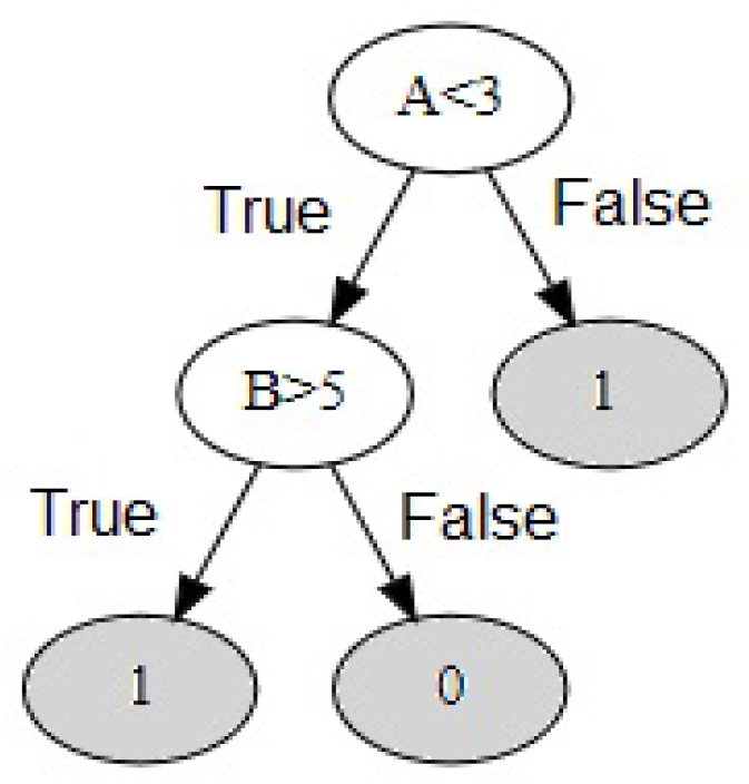
In the context of ML, DT is a directed rooted tree, whose non-leaf nodes correspond to conditions on attributes of a dataset and leaves correspond to the outcomes. The outgoing edges of each non-leaf node are labeled with $True$ and $False$ meaning whether or not the condition associated with that node is satisfied. Thus each edge is associated with a condition which is either condition associated with its tail or the negation of this condition.

The semantics of DT is tied to its root-leaf paths. Each such a path P is seen as the set of conditions $Con{d}_1,\dots ,Con{d}_q$ associated with the edges of P plus the outcome $out$ associated with the leaf. Thus each root-leaf path P of DT can be seen as a rule of the form $Con{d}_1\wedge \cdots \wedge Con{d}_q\to out$, where $Con{d}_1\wedge \cdots \wedge Con{d}_q$ is the body of the rule consisting of conjunctions of individual conditions and $out$ is the outcome of the rule.

The procedure of turning a DT into a set of rules as described above is called linearization. For example, the rules corresponding to the DT in Figure 1 are the following: $(A<3)\wedge (B>5)\to 1$; $(A<3)\wedge (B\le 5)\to 0$; $(A\ge 3)\to 1$.

We use a standard DT algorithm provided by the ML Python library Scikit-Learn [36], with the Gini index served as the splitter and the DT depth is upper-bounded by 7. To obtain a set of rules the resulting DT is linearized. For failure prediction we have two types of outcome only: $out=1$ associated with a failure and $out=0$ otherwise. We record only those rules whose outcome is 1. In other words, we ignore the rules with outcome 0 explaining why a particular failure does not occur because these rules are simply not relevant for our task.

Choice of parameters. As specified in the previous section, the RSC algorithm requires setting of three parameters: $init\_free,init\_prec,prec\_loss$. In all of our experiments, we set these parameters to $1,1\%,0.5\%$ respectively.

The rest of the section consists of two subsection. In each subsection we consider a particular domain and compare our RSC approach with the DT based and SeCo rule learners using this domain.

3.1. Learning the Truth Table of the Given Collection of Rules

Any function on finite domain variables can be defined using a truth table. The truth table consists of all possible tuples of assignment of variables with their domain values, and each tuple is associated with the respective value of the function.

In our first experiment we randomly generate a small collection of small rules, then randomly select a subset S of rows of the truth table of the collection. Next, we run a RL algorithm (RSC, SeCo, and a DT based rule learner) on S with the goal to create a collection of rules as close as possible matching the original one.

The rest of the subsection is organized as follows.

• We define a truth table for a collection of rules.
• We specify an algorithm for generalization of a random collection of rules and of a random subset of its truth table.
• We describe the tests that we performed and their results.

Truth table for a collection of rules and the induced function.

A collection of rules can be associated with many truth tables. This is because, in addition to the variables of the rules, the truth table can also contain many variables that are not essential for the rule. However, since the RL algorithm does not ‘know’ that these extra variables are not essential, these variables make the RL task more difficult.

For example, consider a single rule consisting of a single AVP $(x_1,[2,4])$. A truth table for this rule may consist of 100 variables $x_1,\dots ,x_{100}$. The domain of each variable can be e.g., $\{1,\dots ,10\}$. However, the value of the respective function is determined only by the above AVP: it is 1 if the value of $x_1$ is between 2 and 4, and 0 otherwise.

Having in mind the above example, we give below a formal definition of a truth table for a collection of rules. As an intermediate notion we also define a function induced by the collection of rules, a notion that we will use for the description of a training set.

Definition 8.

Let $\mathbf{C}$ be a collection of rules. Let X be the set of variables of $\mathbf{C}$. For each $x\in X$, let $val\left(x\right)$ be the set of values of X used in the rules of $\mathbf{C}$. Let $X^{*}$ be a set of variables such that $X\subseteq X^{*}$. For each $x\in X^{*}$, the domain $dom\left(x\right)$ of x is defined under the following constraint: if $x\in X$ then $val\left(x\right)\subseteq dom\left(x\right)$. Otherwise, $dom\left(x\right)$ is an arbitrary finite set. Then a function f induced by $\mathbf{C}$ is defined as follows. The domain of f is $X^{*}$. Let $X^{*}=\{x_1,\dots ,x_n\}$. Let $va{l}_1,\dots ,va{l}_n$ be the tuple of assignments to the respective variables. If this tuple is covered by at least one rule of $\mathbf{C}$ then the corresponding value of f is 1, otherwise it is 0.

Given $X^{*}$ and their domains as above, the truth table of $\mathbf{C}$ becomes the truth table of f. That is the rows of the table correspond to the $x_1,\dots ,x_n$ and the last column is for the outcome. The rows of the table are all the tuples of assignments to $X^{*}$ and their corresponding value of f as described above.

Generation of a random collection of rules and a random subset of the related truth table.

• Choose the following parameters.

  (a)

  $num\_attr$, the number of attributes.

  (b)

  $max\_val$, the largest value for each attribute meaning that the attribute values will lay in the interval $[0,max\_val]$.

  (c)

  $num\_rules$, the number of rules to be generated.

  (d)

  $len\_rule$, the length of the generated rules

  (e)

  $num\_rows$, the number of rows of the training set.

• Randomly generate a collection of $\mathbf{C}$ having number of rules $num\_rules$. Each rule is a random generation of $len\_rule$ AVPs that can be done as follows.

  (a)

  Randomly choose $len\_rule$ attributes for the given rule.

  (b)

  For each chosen attribute $attr$, randomly generate an interval $[a,b]$ such that $0\le a\le b\le max\_val$ and the resulting AVP is $(attr,[a,b\left]\right)$.

• Randomly generate $num\_rows$ of the ‘truth’ table for the above rules in order to create a training set. A row of the truth table is generated as follows.

  (a)

  Randomly generate a value for each attribute between 0 and $max\_val$.

  (b)

  Let $tp$ be the resulting tuple of attribute values.

  (c)

  If $tp$ is covered by $\mathbf{C}$ then $out=1$, otherwise $out=0$.

  (d)

  Add $out$ in the last column of $tp$.

To make the work of a rule learner more complicated, we also generate rows by introducing a random noise. In order to do this, we choose a small parameter $noise\_prob$ (e.g., $0.005$) and then, in the above algorithm, after having computed the outcome, alter it with probability $noise\_prob$.

Example 3 demonstrates the experiment.

Example 3.

Suppose $max\_val=1$ that means that all the attribute values are binary: 0 or 1. Moreover, this also means that the collection of rules become Disjunctive Normal Forms (DNFs).

Then $num\_rules$ becomes the number of conjuncts and $len\_rule$ becomes the length of the conjuncts. Suppose that both of them equal 2. Let the collection of rules be $(x_1\wedge x_2)\vee (x_3\wedge x_4)$. Let also the number of attributes be 10. Thus we have defined the function $f(x_1,\dots ,x_{10})=(x_1\wedge x_2)\vee (x_3\wedge x_4)$. The whole dataset is just the truth table of this function. The $num\_rows$ parameter is the size of the training set (seen by the algorithm). These $num\_rows$ rows are randomly selected out of the whole dataset. A RL algorithm is supposed to guess the whole function out of these rows.

Testing and analysis of the results.

Now, suppose a RL algorithm returns a collection of rules g. How can we determine the closeness of g to the function f induced by the collection of rules? The truth table of g consists of the same tuples as the truth table of f (but the values of the function can, of course be different). Therefore, we proceed as follows.

• Calculate the numbers of rows that are satisfied by f, g and $f\wedge g$ (both g and f) and denote them by $\left|f\right|$, $\left|g\right|$ and $|f\wedge g|$, respectively.
• The number $|f\wedge g|/\left|f\right|$ is the percent of rows covered by f that are also covered by g. The larger this number the better is the quality of the learned model.
• The number $|f\wedge g|/\left|g\right|$ is the percent of rows covered by g that are also covered by f. The larger this number the smaller the number of rows of g that are not covered by f and the better the quality of g.

Note that the computation of the number of rows is in general an intractable problem. However, since we consider small collections of small rules this can be done by a brute-force algorithm.

We test the algorithms (RSC, SeCo, and DT) in the modes specified by the following parameters.

• The number of extra variables. Extra variables are those that do not take part in the rules of f. They are inessential, however their presence can seriously hinder performance of an RL algorithm. Getting rid of such variables is the main task of the feature selection algorithm. We consider two extreme modes: few extra variables and many extra variables. We gradually increase the number of variables in order to see a point where the rule learner starts to work much worse. In case of many variables, the performance can be significantly improved with the introduction of feature selection algorithms. However, in this experiment we want to see how the algorithm deals alone with this matter.
  Having many variables has another interesting feature: the size of the truth table becomes very large (100 variables with domain 2 in each of them result in a truth table of $2^{100}$ rows). This means that a training set (in which rows are explicitly presented) becomes tiny compared to the whole truth table. It is interesting to see how an RL algorithms would cope with this situation.
• The number of extra values. Suppose x is a variable occurring in the rules of f. However, the domain of x may contain many values that do not take part in any interval of an AVP of x in f. When there are many additional values, the event of the function f equal 1 becomes rare and hence it is more difficult for a rule learner to ‘spot’ the rule. We will check truth tables with few and with many background values.

Thus the options of few/many extra variables and few/many extra values give us 4 modes of testing combined. If we add presence/absence of random noise this will make 8 modes of testing in total.

We perform experiments according to the above classification. Our conclusions based on these experiments are summarized below.

• Small number of extra variables. In this case the RSC algorithm correctly reconstructs the original function. However, if we increase the number of values, the algorithm splits the original rules so the number of resulting rules is larger than the number of the original rules. The effect of splitting can be demonstrated on the following example. Consider a rule $(x_1,[1,10])\wedge (x_2,[1,10])$. As a result of splitting this rule can be represented by the following collection of four rules $\{[x_1,[1,5])\wedge (x_2,[1,5])$, $(x_1,[1,5])\wedge (x_2,[6,10])$, $(x_1,[6,10])\wedge (x_2,[1,5])$, $(x_1,[6,10])\wedge (x_2,[6,10])\}$
  The larger the intervals the stronger output of our algorithm is affected by splitting. This effect can be alleviated by using non-zero $prec\_loss$ parameter, for instance, about half percent ($prec\_loss$ is defined for the function $IsReplaces$ in Algorithm 3 in Section 2). As a result of this, the algorithm is ‘encouraged’ to move to a larger interval even if the resulting precision is slightly smaller. However, the fragmentation of the rules still exists. We believe this can be addressed by a post-learning algorithm that tries to simplify the already created rules [4]. This is an interesting topic for future research.
• Many extra variables. In this case, the RSC algorithm has tendency to include irrelevant variables into the rules. This inclusion has an interesting side effect: redundant variables in correct rules. For example, suppose we have a rule $[x_1,[1,5])\wedge (x_2,[1,5])$. If the number of variables is say 100 and the size of the sample of the truth table considered by the algorithm is say 1000 (tiny proportion of total number of $2^{100}$ of the truth table) then there might be some irrelevant variable with an interval whose precision is better then any interval of $x_1$ or $x_2$. In this case the algorithm picks something like $(x_{10},[1,2])$ and then a relevant variable. This effect makes the collection of rules longer than needed. Still, in the vast majority of cases, the function of the collection of rules formed was exactly the function of the original rules.
  In about $1\%$ of cases, we obtained rules with false positives. The reason for that is an effect of ‘shadowing’: when a training set is so tiny compared to the ‘full’ data, some statistical ‘anomalies’ are possible. For example, it may happen that an interval of an irrelevant variable perfectly correlates with the rows where the function is 1. Clearly, in this case, the algorithm will pick the correlating interval of an irrelevant variable.
  The above situation can be fixed if the algorithm considers several random training sets of the same size. This allows the ‘stray’ irrelevant variable to be ‘shaken off’.
  If in additional to many extra variables some relevant variables contain many extra values, the negative effects specified above are, of course moderately aggravated. For instance, the RSC algorithm did not manage to correctly guess the function only in about 3% of cases.
• The influence of noise. The noise does not significantly affect the behavior of the algorithm as specified above. In particular, the RSC algorithm is still able to recognize the main rules and does not try to ‘collate’ the ‘noisy’ rows with the main ones.
• Comparison of RSC with DT based and Separate-and-Conquer (SeCo) rule learners. Finally, it is important to say that on this domain the RSC algorithm works much better than the DT and SeCo (with $ChooseNext$ heuristic) rule learners.
  Indeed, in those rare cases where RSC returns an incorrect collection of rules, the difference between the output and the original collection of rules has never been more than 2%. On the other hand, the rules returned by the DT based rule learner even in case of few extra variables and small domains are at least $20\%$ different from the original collection of rules. In case of many extra variables, the difference can be up to $40\%$. The SeCo (with $ChooseNext$ heuristic) is only marginally better than DT.
  A typical situation when both DT and SeCo fail to discover the right set of rules can be described by the following simple example. Suppose that the dataset consists of 10 attributes $att{r}_1,\dots ,att{r}_{10}$, each attribute can take values $1,\dots ,5$ and the outcome is 1 only for rows covered by one of the following two rules.

  (a)

  $att{r}_1\in [1,4]\wedge att{r}_4\in [2,5]$

  (b)

  $att{r}_2\in [1,3]\wedge att{r}_3\in [3,5]$

  Both RSC and SeCo easily discover the first rule. RSC quickly discovers the second rule. However, the SeCo rule have been removed. It picks an unrelated variable and then creates many irrelevant rules just to cover the remaining rows. Unsurprisingly, on the testing set such rules are far from being accurate.

3.2. Failure Prediction Using a Real Industrial Dataset

For our experiments we use a real industrial dataset collected from a machine which manufactures the plastic bottle caps. This dataset consists of two following parts.

The first part is a collection of tuples of sensor readings provided in CSV format that have been collected over more than one year from this machine. Each tuple of sensor readings is associated with a timestamp. We create a table R with columns (attributes) corresponding to the sensors and the rows being the tuples of corresponding readings. To make connection with the second part of the data, we also keep the timestamps of the tuples in the memory.

The second part is information about alarms. This data consists of tuples having three components: start and end timestamps of an alarm and alarm error code. The alarms are associated with failures in this industrial machine, in the sense that if an alarm occurs, the machine should be switched off to find the failure. The alarm error codes are organized into four groups: shutdown, stoppage, mandatory action and message. The first two groups (shutdown and stoppage) are main errors that should be predicted to prevent failures in the machine. Five types of shutdown and stoppage alarms happen most often. In this section we refer to them by index $i\in \{1,2,3,4,5\}$ for the purpose of explanation.

The rest of this subsection is divided into the following four parts.

• Testing the ability of the considered algorithms to predict the actual alarms occurring at the given moment of time.
• Testing the remaining useful life prediction (RUL), this is effectively the ability to predict an alarm to occur in the near future.
• Testing the true and false positive rates.
• Making conclusion based on the obtained empirical results.

Prediction of actual alarms.

For all alarms, we form the respective datasets $D_1,\dots ,D_5$. Each $D_i$ is formed as follows.

• We take the table R created from the first part of the dataset and add to it one extra column $out$.
• For each row of R, we check whether alarm i occurred at the moment of the timestamp associated with the row. If it did, the value of $out$ in this row is set to 1. Otherwise, the value of $out$ is set to 0.

As a result, we obtain datasets where the sensor readings serve as attributes and the values of the last column serve as outcomes.

We perform the experiments for RSC, DT based and SeCo (with $ChooseNext$ heuristic) algorithms as follows.

• We run the algorithm for each $D_i$ separately. For this, we randomly partition the rows of $D_i$ into the training ($70\%$ of the rows) and testing sets ($30\%$ of the rows), and record all the rules.
• Each rule is tested on the testing set corresponding to the predicted alarm. That is, for the predicted alarm i any rule obtained from the the training set of $D_i$ is tested on the testing set of $D_i$. For each rule, we record its precision with respect to the testing set (see Definition 5).
• We record together the rules obtained from the exploration of all datasets $D_1,\dots D_5$, replacing the outcome 1 with the respective real alarm code, and remove those rules that cover less than 20 lines in the dataset as insignificant.

Some rules and their precision are reported in

Table 1. Relaxed Separate-and-Conquer (RSC) (RUL = 0 s).

Alarm	Rules	Precision
$1017$	$(\%ZP=0)\wedge (Ads.HmiVis.EXTR.PRESS\_I\in [8.63,170.95\left]\right)$	$98\%$
	$(\%ZP=0)\wedge (TEMP\_E_1\in [185.73,194.97])$	$95\%$
$3042$	$(TEMP\_CI\in [49.6,50.1])\wedge (TEMP\_E_{10}\in [164.76,199.1])\wedge (TEMP\_ZP\in [21.4,184.8])$	$96\%$
	$(TEMP\_CI\in [49.6,50.1])\wedge (PRES\_PI\in [0,0.8])\wedge (\%E_1\in [-33.34,15.1])$	$97\%$
	$(Ads.HmiVis.CCM.CORSA\_AP\in [113.3,114.5\left]\right)\wedge (TEMP\_CI\in [21.7,42\left]\right)\wedge (TEMP\_PI\in [26,31\left]\right)$	$96\%$
$3167$	$(\%E_2\in [-5,4.07])\wedge (Ads.HmiVis.CENTR.PRESS\_B\in [0.2,69.8])\wedge (TEMP\_PI\in [12.9,20.6])$	$97\%$
	$(TEMP\_E_1\in [170.53,195.02])\wedge (TEMP\_PI\in [26.1,31])\wedge (TEMP\_E_4\in [180,197.1])$	$94\%$
$3197$	$(TEMP\_PS\in [36.88,37.3\left]\right)\wedge (Ads.HmiVis.EXTR.PRESS\_I\in [7.83,170.8\left]\right)$	$96\%$
	$(TEMP\_PS\in [36.9,37.3\left]\right)\wedge (\%CU\in [24.77,100\left]\right)$	$98\%$
	$(\%PS\in [40.55,100\left]\right)\wedge (Ads.HmiVis.EXTR.PRESS\_I\in [17.58,161.93\left]\right)$	$97\%$
$3099$	$(Ads.HmiVis.CENTR.POT\_M1B\in [75.7,78.3])\wedge (\%E_5\in [-8.1,6.4])\wedge (\%E_1\in [-33.4,29.4])$	$93\%$
	$(Ads.HmiVis.CENTR.POT\_M1B\in [58.8,78.3\left]\right)\wedge (TEMP\_CI\in [21.7,28.5\left]\right)\wedge (\%TB\in [0,15.4\left]\right)$	$96\%$

for RSC, in

Table 2. Decision Tree (DT) based rule learner (RUL = 0 s).

Alarm	Rules	Precision
$1017$	$(TEMP\_E_2>178.79)\wedge (\%ZP<=2.46)\wedge (\%TB<=4.3)$	$89\%$
$3042$	$(TEMP\_CI>47.55)\wedge (TEMP\_ST<=49.15)\wedge (PORT\_PS>0.8)\wedge (TEMP\_E_5>158.35)\wedge (TEMP\_FU<=167.2)$	$90\%$
	$(TEMP\_CI>47.55)\wedge (TEMP\_ST<=49.15)\wedge (PORT\_PS<=0.8)\wedge (\%E_2<=11.125)\wedge$ $(Ads.HmiVis.EXTR.PRESS\_O<=15.76)\wedge (Ads.HmiVis.CENTR.PRESS\_B<=15.03)$	$89\%$
$3167$	$(Ads.HmiVis.CCM.CORSA\_AP>114.22)\wedge (TEMP\_PS<=25.92)\wedge (TEMP\_CI<=44.95)\wedge$ $\wedge (Ads.HmiVis.CENTR.PRESS\_B>0.17)\wedge (\%TB<=17.01)$	$94\%$
	$(Ads.HmiVis.CCM.CORSA\_AP>114.34)\wedge (TEMP\_PS<=25.92)\wedge (TEMP\_CI<=44.95)\wedge$ $\wedge (Ads.HmiVis.CENTR.PRESS\_B<=0.17)\wedge (Ads.HmiVis.EXTR.PRESS\_O<=14.36)\wedge (TEMP\_PI>18.26)\wedge$ $(Ads.HmiVis.EXTR.PRESS\_I>7.4)$	$88\%$
$3197$	$(TEMP\_PS>36.89)\wedge (Ads.HmiVis.EXTR.PRESS\_I>5.57)\wedge \%PI>-4.69)$	$92\%$
	$(TEMP\_PS>36.89)\wedge (Ads.HmiVis.EXTR.PRESS\_I<=5.57)\wedge (Ads.HmiVis.EXTR.PRESS\_O>5.62)$	$91\%$
$3099$	$(\%PS>40.7)\wedge (Ads.HmiVis.CENTR.POT\_M1B>61.1)$	$94\%$

for a DT based rule learner and in

Table 3. Separate-and-Conquer (SeCo) (RUL = 0 s).

Alarm	Rules	Precision
$1017$	$(\%UG\in [0.87,6.19])\wedge (Ads.HmiVis.CENTR.PRESS\_B\in [4.11,65.78])\wedge (TEMP\_E_2\in [175.8,192.32])$	$93\%$
	$(\%ZP=0)\wedge (TEMP\_E_1\in [185.73,194.97])\wedge (\%E_6\in [-12.3,25.71])\wedge (Ads.HmiVis.CENTR.POT\_M1B\in [54.62,81.78])$	$90\%$
$3042$	$(PRES\_PI\in [0.3,4.2])\wedge (\%E_1\in [-20.17,5.75])\wedge (TEMP\_E_{10}\in [170.19,187.16])\wedge (TEMP\_ZP\in [27.46,189.15])$	$91\%$
	$(PRES\_PI\in [0,3.89])\wedge (\%E_1\in [-24.8,8.3])\wedge (\%E_2\in [-37.89,12.21])\wedge \%E_4\in [-20.12,15.33])$	$93\%$
	$(TEMP\_CI\in [49.6,50.1])\wedge (PRES\_PI\in [0.67,4.07])\wedge (\%E_3\in [-32.64,17.43])\wedge (TEMP\_FL\in [175.4,199.4])$	$92\%$
	$(Ads.HmiVis.CCM.CORSA\_AP\in [113.78,114.85\left]\right)\wedge (TEMP\_CI\in [22.42,44.86\left]\right)\wedge (TEMP\_PI\in [27.41,37.16\left]\right)\wedge$ $(Ads.HmiVis.CENTR.PRESS\_B\in [15.46,65.85\left]\right)$	$90\%$
$3167$	$(\%E_1\in [173,184.3])\wedge (\%E_2\in [-15.8,24.52])\wedge (Ads.HmiVis.CENTR.PRESS\_B\in [0.14,25.7])\wedge$ $(TEMP\_PI\in [24.49,32.6])\wedge (TEMP\_E_1\in [178.5,193.02])\wedge (TEMP\_E_4\in [180.55,199.51])$	$94\%$
$3197$	$(TEMP\_PS\in [35.79,38.13\left]\right)\wedge (Ads.HmiVis.EXTR.PRESS\_I\in [4.63,169.18\left]\right)\wedge (\%CU\in [28.23,96.74\left]\right)\wedge$ $(Ads.HmiVis.EXTR.PRESS\_0\in [17.25,148.32\left]\right)$	$91\%$
	$(TEMP\_PS\in [37.35,38.69\left]\right)\wedge (Ads.HmiVis.EXTR.PRESS\_I\in [5.92,172.5\left]\right)\wedge (\%CU\in [24.77,100\left]\right)\wedge$ $(Ads.HmiVis.CENTR.POT\_M1B\in [71.48,77.84\left]\right)\wedge (TEMP\_CI\in [20.43,29.94\left]\right)$	$93\%$
	$(\%PS\in [40.55,100\left]\right)\wedge (Ads.HmiVis.CENTR.POT\_M1B\in [74.75,79.18\left]\right)\wedge (Ads.HmiVis.EXTR.PRESS\_O\in [3.74,12.5\left]\right)$ $\wedge (Ads.HmiVis.EXTR.PRESS\_I\in [17.58,161.93\left]\right)$	$90\%$
$3099$	$(Ads.HmiVis.CENTR.POT\_M1B\in [75.7,78.3\left]\right)\wedge (TEMP\_CI\in [22.25,26.29\left]\right)\wedge (\%TB\in [1.75,13.16\left]\right)\wedge$ $(\%E_5\in [-8.1,6.4])\wedge (\%E_1\in [-33.4,29.4])$	$90\%$
	$(TEMP\_PS\in [32.41,39.79\left]\right)\wedge (Ads.HmiVis.EXTR.PRESS\_I\in [12.97,167.17\left]\right)\wedge (TEMP\_CI\in [21.7,28.5\left]\right)\wedge$ $(\%TB\in [0,15.4\left]\right)\wedge (\%PS\in [44.17,96.51\left]\right)$	$93\%$

for SeCo. Each row in the tables corresponds to a rule. The first column ‘alarm’ states the predicted alarm code. The second column ‘rules’ describes the body of the rule, we grouped several rules predicting the same alarm. For example, the rule on the first row of Table 1 should be interpreted as follows. If the value of the attribute $\%ZP$ is 0 and the value of the attribute $Ads.HmiVis.EXTR.PRESS\_I$ is in the interval [8.63,170.95] then alarm 1017 occurs. The rule on the last row of Table 2 is interpreted as follows. If the value of the attribute $\%PS$ is greater than $40.7$ and the value of the attribute $Ads.HmiVis.CENTR.POT\_M1B$ is greater than 61.1 then alarm 3099 occurs. The last column ‘precision’ measures how much the given rule is precise for the dataset, calculating the percentage of rows of the testing set on which the alarm actually occurs among those covered by the respective rule (as in Definition 5).

Let us make one interesting remark. The rules generated by the above algorithms are overlapping in the sense that a row of table R can be covered by more than one rule meaning that the set of rules predict that more than one alarm is taking place during the corresponding timestamp. This means that two or more alarms may occur simultaneously. In fact, classifying each alarm separately is a standard ML approach for multiple classification tasks. It is called unordered rules and there is evidence that this approach makes more accurate predictions than learning mutually exclusive rules, see e.g., [37].

RUL prediction.

We also test the ability of algorithms to predict the remaining time to failure (or RUL - remaining useful life). In particular, for a time t seconds, we modify tables $D_1,\dots ,D_5$ to obtain the respective tables $D_1^t,\dots ,D_5^t$ as follows. Take table $D_i$ and set the $out$ column to 1 in those rows whose timestamp is at most t seconds before the timestamp of a row having $out=1$ in $D_i$. The resulting table is $D_i^t$. We report experiments with two values of t: 60 and 120, chosen for the sake of demonstration. The resulting rules and the testing results of the respective RSC, DT based and SeCo algorithms are reported in

Table 4. Relaxed Separate-and-Conquer (RSC) (RUL = 60 s).

Alarm	Rules	Precision
	$(TEMP\_E_4\in [182.5,197.1])\wedge (\%ZP=0)$	$96\%$
$1017$	$(\%UG\in [0,7.59\left]\right)\wedge (TEMP\_PI\in [12.9,19.6\left]\right)$	$95\%$
	$(TEMP\_CI\in [49.6,50.1])\wedge (\%E_5\in [-8.08,12.72])$	$97\%$
$3042$	$(TEMP\_CI\in [47.9,50.1\left]\right)\wedge (\%UG\in [0,13.25\left]\right)\wedge (\%FL\in [0,5.95\left]\right)$	$93\%$
	$(Ads.HmiVis.CCM.CORSA\_AP\in [114.09,114.52\left]\right)\wedge (TEMP\_CI\in [40.5,42\left]\right)$	$95\%$
$3167$	$(TEMP\_E_1\in [170.6,194.9])\wedge (TEMP\_PI\in [26.1,31])\wedge (TEMP\_E_2\in [174,196.6])$	$94\%$
	$(TEMP\_PS\in [36.82,37.3\left]\right)\wedge (Ads.HmiVis.EXTR.PRESS\_I\in [7.8,172.47\left]\right)$	$93\%$
$3197$	$(TEMP\_PS\in [36.82,37.3])\wedge (\%E_2\in [4.58,100])$	$95\%$
	$(TEMP\_CI\in [21.7,37.2\left]\right)\wedge (TEMP\_ST\in [54.4,61.2\left]\right)$	$90\%$
$3099$	$(\%PS\in [45.03,100\left]\right)\wedge (\%PI\in [-100,-62.01\left]\right)$	$91\%$
	$(TEMP\_CI\in [21.7,28.5\left]\right)\wedge (Ads.HmiVis.EXTR.PRESS\_O\in [4.8,133\left]\right)\wedge (\%ZF\in [10.2,100\left]\right)$	$89\%$

,

Table 5. Decision Tree (DT) based rule learner (RUL = 60 s).

Alarm	Rules	Precision
$1017$	$(TEMP\_E_4>182.45)\wedge (\%UG>8.84)\wedge (TEMP\_E_{10}<=193.86)$	$88\%$
	$(TEMP\_E_4>182.45)\wedge (\%UG<=8.84)\wedge (\%ZP<=10.08)$	$90\%$
	$(TEMP\_CI>47.65)\wedge (TEMP\_ST>49.25)\wedge (TEMP\_PS<=23.85)\wedge (\%E_5<=12.89)\wedge (TEMP\_FU<=180)$	$88\%$
$3042$	$(TEMP\_CI<=47.65)\wedge (\%CU>29)\wedge (\%E_2<=5.64)\wedge (\%E_3>2.17)$	$85\%$
	$(TEMP\_CI>47.65)\wedge (TEMP\_ST<=49.25)\wedge (TEMP\_E_4<=166.05)\wedge (\%E_4<=13.54)\wedge (\%FL<=21.73)$	$91\%$
$3167$	$(TEMP\_PS<=26.15)\wedge (Ads.HmiVis.CCM.CORSA\_AP<=114)\wedge (TEMP\_E_1>170.54)\wedge (TEMP\_PI>26.08)$	$93\%$
	$(TEMP\_PS<=26.15)\wedge (Ads.HmiVis.CCM.CORSA\_AP>114)\wedge (TEMP\_CI<=44.95)\wedge (\%E_1<=43.57)\wedge$ $(Ads.HmiVis.CENTR.PRESS\_B>0.18)$	$92\%$
$3197$	$(TEMP\_PS>36.85)\wedge (TEMP\_ST>57.95)\wedge (Ads.HmiVis.EXTR.PRESS\_I>5.57)\wedge (\%E_1>8.37)\wedge (\%FL>6.98)$	$89\%$
	$(TEMP\_PS>36.85)\wedge (TEMP\_ST>57.95)\wedge (Ads.HmiVis.EXTR.PRESS\_I<=5.57)\wedge (\%E_4<=5.78)$	$85\%$
$3099$	$(\%PS>41.15)\wedge (Ads.HmiVis.CENTR.POT\_M1B>58.78)\wedge (TEMP\_FU>182.1)$	$90\%$

and

Table 6. Separate-and-Conquer (SeCo) (RUL = 60 s).

Alarm	Rules	Precision
	$(TEMP\_E_1\in [167.75,193.43])\wedge (TEMP\_E_4\in [180.43,194.98])\wedge (TEMP\_PI\in [10.15,17.34])$	$93\%$
$1017$	$(\%UG\in [0.9,9.13])\wedge (TEMP\_E_1\in [166.12,196.57])\wedge (TEMP\_CI\in [44.76,52.21])\wedge (TEMP\_PI\in [11.69,18.51])$	$89\%$
	$(TEMP\_CI\in [45.6,53.72])\wedge (TEMP\_E_2\in [174,196.6])\wedge (\%FL\in [0.8,7.98])\wedge (\%E_5\in [-12.61,17.54])$	$90\%$
$3042$	$(TEMP\_CI\in [48.21,54.66])\wedge (\%E_2\in [-10.62,18.04])\wedge (\%UG\in [0.98,10.15])\wedge (\%FL\in [1.13,10.65])$	$92\%$
	$(Ads.HmiVis.CCM.CORSA\_AP\in [116.76,121.39\left]\right)\wedge (TEMP\_CI\in [37.18,43.76\left]\right)\wedge$ $(Ads.HmiVis.CENTR.PRESS\_B\in [3.32,20.23])\wedge (TEMP\_E_6\in [173.74,199.32])$	$91\%$
$3167$	$(TEMP\_E_1\in [174.57,195.28])\wedge (\%E_3\in [-10.72,18.65])\wedge (TEMP\_PI\in [22.18,33.78])\wedge (TEMP\_E_2\in [168.76,189.25])$	$88\%$
	$(Ads.HmiVis.CENTR.PRESS\_A\in [10.74,22.86\left]\right)\wedge (Ads.HmiVis.EXTR.PRESS\_I\in [14.97,162.83\left]\right)\wedge$ $(TEMP\_PS\in [30.35,39.71\left]\right)$	$90\%$
$3197$	$(TEMP\_PS\in [31.73,35.12])\wedge (TEMP\_CI\in [40.81,58.54])\wedge (\%E_4\in [31.72,73.18])\wedge$ $(Ads.HmiVis.EXTR.PRESS\_I\in [15.14,178.52\left]\right)\wedge (TEMP\_PI\in [10.86,22.86\left]\right)$	$91\%$
	$(TEMP\_CI\in [19.83,41.45\left]\right)\wedge (Ads.HmiVis.EXTR.PRESS\_I\in [17.89,65.71\left]\right)\wedge (TEMP\_ST\in [50.07,82.13\left]\right)$	$92\%$
$3099$	$(\%PS\in [78.13,80.54\left]\right)\wedge (\%PI\in [-75.34,-12.53\left]\right)\wedge (Ads.HmiVis.EXTR.PRESS\_O\in [21.75,87.35\left]\right)\wedge (\%ZF\in [13.65,94.5\left]\right)$	$93\%$

for $RUL=60$ s and in

Table 7. Relaxed Separate-and-Conquer (RSC) (RUL = 120 s).

Alarm	Rules	Precision
$1017$	$(TEMP\_E_4\in [182.47,197.1])\wedge (\%ZP=0)$	$91\%$
	$(\%UG\in [0,7.61])\wedge (TEMP\_FL\in [187.4,199.3])\wedge (\%E_1\in [-32.79,0])$	$95\%$
$3042$	$(TEMP\_CI\in [48.5,50.1])\wedge (TEMP\_E_5\in [21.2,165.5])\wedge (\%E_1\in [-33.34,12.81])$	$96\%$
	$(TEMP\_CI\in [49.4,50.1])\wedge (\%E_4\in [-6.65,12.14])$	$94\%$
$3167$	$(Ads.HmiVis.CCM.CORSA\_AP\in [113.8,114.5\left]\right)\wedge (TEMP\_CI\in [21.7,42.1\left]\right)$	$91\%$
	$(TEMP\_E_2\in [175.4,196.9])\wedge (TEMP\_E_1\in [169.9,195])\wedge (TEMP\_PI\in [26.1,31])$	$95\%$
$3197$	$(TEMP\_PS\in [36.8,37.3])\wedge (\%E_2\in [4.57,100])$	$94\%$
	$(TEMP\_E_1\in [21.3,164.9])\wedge (Ads.HmiVis.CCM.CORSA\_AP\in [113.47,114.52])$	$96\%$
$3099$	$(TEMP\_CI\in [21.7,40.5\left]\right)\wedge (TEMP\_PS\in [17.8,25.3\left]\right)$	$92\%$
	$(\%UG\in [19.73,100])\wedge (TEMP\_CU\in [184.4,188.8])\wedge (\%E_3\in [5.49,100])$	$96\%$
	$(\%FL\in [7.99,8.17\left]\right)\wedge (TEMP\_CI\in [21.7,28.5\left]\right)$	$94\%$

,

Table 8. Decision Tree (DT) based rule learner (RUL = 120 s).

Alarm	Rules	Precision
$1017$	$(TEMP\_E_4>182.56)\wedge (\%UG<=9.67)\wedge (TEMP\_E_5>181.58)$	$89\%$
	$(TEMP\_CI>47.55)\wedge (TEMP\_ST<=49.25)\wedge (\%E_4<=13.59)\wedge (TEMP\_PI>21.09)$	$90\%$
$3042$	$(TEMP\_CI<=47.55)\wedge (\%CU<=30.14)\wedge (\%ZP>15.55)\wedge (TEMP\_E_9<=164.66)$	$88\%$
	$(TEMP\_CI<=47.55)\wedge (\%CU>30.14)\wedge (\%E_2<=4.74)\wedge (Ads.HmiVis.EXTR.PRESS\_I<=10.38)$	$89\%$
	$(TEMP\_PI>26.08)\wedge (Ads.HmiVis.CCM.CORSA\_AP<=114.48)\wedge (TEMP\_E_1>170.59)\wedge (TEMP\_E_4>179.15)$	$91\%$
$3167$	$(TEMP\_PI>26.08)\wedge (Ads.HmiVis.CCM.CORSA\_AP>114.48)\wedge (TEMP\_PS<=25.9)\wedge$ $(TEMP\_CI<=44.95)\wedge (TEMP\_E_7>184.75)$	$90\%$
	$(Ads.HmiVis.EXTR.PRESS\_I>5.56)\wedge (Ads.HmiVis.EXTR.PRESS\_O<=5.79)\wedge (TEMP\_PS>36.75)\wedge$ $(\%CU>22.87)\wedge (Ads.HmiVis.CENTR.PRESS\_B>0.22)\wedge (\%ZF<=8.38)$	$92\%$
$3197$	$(Ads.HmiVis.EXTR.PRESS\_I>5.56)\wedge (Ads.HmiVis.EXTR.PRESS\_O<=5.79)\wedge (TEMP\_PS>36.75)\wedge$ $(\%CU<=22.87)\wedge (TEMP\_FU<=183.96)$	$91\%$
$3099$	$(\%PS>40.55)\wedge (Ads.HmiVis.CENTR.POT\_M1B>58.68)\wedge (\%ZP<=11.93)$	$93\%$

and

Table 9. Separate-and-Conquer (SeCo) (RUL = 120 s).

Alarm	Rules	Precision
$1017$	$(TEMP\_E_1\in [173.52,195.67])\wedge (TEMP\_E_2\in [167.13,183.73])\wedge (\%E_5\in [-26.15,3.75])\wedge (\%ZP\in [0,74,2.69])$	$89\%$
	$(\%UG\in [0.3,9.62])\wedge (TEMP\_FL\in [176.86,197.81])\wedge (\%E_1\in [-35.7,0.76])\wedge (\%E_2\in [-40.35,1.6])$	$93\%$
$3042$	$(TEMP\_CI\in [42.19,53.9])\wedge (TEMP\_E_1\in [36.81,112.52])\wedge (\%E_3\in [-38.7,17.51])\wedge (TEMP\_PS\in [22.5,36.51])$	$92\%$
	$(TEMP\_CI\in [47.4,58.42])\wedge (\%UG\in [40.19,88.61])\wedge (\%E_3\in [-15.8,47.5])\wedge$ $\wedge (TEMP\_PS\in [16.5,42.62])\wedge (\%E_4\in [-18.75,35.9])$	$91\%$
$3167$	$(Ads.HmiVis.CCM.CORSA\_AP\in [109.54,119.83])\wedge (TEMP\_E_7\in [168.9,194.61])\wedge$ $(Ads.HmiVis.CENTR.PRESS\_B\in [6.28,23.75\left]\right)\wedge (TEMP\_CI\in [19.35,38.6\left]\right)$	$90\%$
	$(TEMP\_E_6\in [187.4,192.84])\wedge (Ads.HmiVis.CENTR.PRESS\_A\in [8.86,27.71])\wedge$ $(TEMP\_PI\in [29.82,33.78])\wedge (TEMP\_E_8\in [125.7,186.6])$	$94\%$
$3197$	$(TEMP\_PS\in [33.56,43.68\left]\right)\wedge (Ads.HmiVis.EXTR.PRESS\_I\in [18.76,146.67\left]\right)\wedge$ $(\%E_2\in [7.8,87.4])\wedge (\%E_6\in [3.78,87.92])$	$93\%$
	$(Ads.HmiVis.CENTR.PRESS\_B\in [4.81,84.65])\wedge (\%E_1\in [16.85,86.9])\wedge (TEMP\_CU\in [163.7,193.89])\wedge$ $(\%E_6\in [5.25,76.92])\wedge (Ads.HmiVis.CCM.CORSA\_AP\in [103.87,87.3])\wedge (TEMP\_E_3\in [27.2,136.85])$	$91\%$
$3099$	$(TEMP\_CI\in [22.87,67.85])\wedge (TEMP\_PS\in [7.89,18.82])\wedge (\%UG\in [29.15,74.63])\wedge (\%E_1\in [8.14,77.34])$	$89\%$
	$(\%FL\in [2.96,18.7\left]\right)\wedge (TEMP\_CI\in [24.12,35.9\left]\right)\wedge (TEMP\_CU\in [167.8,191.3\left]\right)$	$88\%$

for $RUL=120$ s.

$\mathit{TP}$ and $\mathit{FP}$ rates.

We also calculate the True Positive ($TP$) and False Positive ($FP$) rates for our experiments. For this task we form the dataset $D=D_1\vee D_2\vee D_3\vee \vee D_4\vee D_5$. That is, if any alarm occurred at the moment of the timestamp associated with each row, $out=1$ in this row, otherwise, $out=0$. We run RSC and DT based rule learner on obtained dataset D for rule generation.

To calculate $TP$ (correct prediction of alarms), we define A as a set of rows associated with any alarm in the testing set of D (having $out=1$) and a as a number of all rows in A. Then $TP=t/a$, where t is the number of such rows of A which are covered by at least one rule. The results are $TP=97\%$ for RSC, $TP=90\%$ for DT based rule learner and $TP=92\%$ for SeCo.

To calculate $FP$ (incorrect prediction of alarms), we define N be a set of rows in the testing set of D which are not associated with any alarm (with $out=0$) and n is the number of all rows in N. Then $FP=f/n$, where f is the number of such rows of N which are covered by at least one rule. We obtain $FP=0.01\%$ for RSC, $FP=0.2\%$ for DT based rule learner and $FP=0.1\%$ for SeCo.

Also, we perform $TP$ and $FP$ calculation on datasets $D^{60}=D_1^{60}\vee \cdots \vee D_5^{60}$ and $D^{120}=D_1^{120}\vee \cdots \vee D_5^{120}$, and obtain similar results. $TP$ and $FP$ calculation are provided in

Table 10. $TP$ and $FP$ calculation.

	RSC	DT Based	SeCo
$TP$	$97\%$	$90\%$	$92\%$
$FP$	$0.01\%$	$0.2\%$	$0.1\%$

.

The proposed algorithm outputs rules predicting alarms (outcome 1). There are no rules making negative predictions (absence of the alarm). As a result, there are no false negative predictions. This, in turn, means that those measures that involve false negatives (TN, FN) do not make sense: for example, the accuracy coincides with the precision and the recall becomes equal 1.

Conclusions of experiments.

Based on the experiments, the following conclusions are reached.

• The levels of precision for individual rules produced by the RSC algorithm are higher than those of DT based and SeCo rule learners.
• The rules produced by RSC are significantly shorter than those produced by DT based and SeCo rule learners.
• The $TP$ rate for RSC algorithm is much higher than that of DT based and SeCo rule learners: on average it is $97\%$ versus $90\%$ and $92\%$, respectively. We attribute this improvement to the shortening of rules.
• The $FP$ rate for RSC algorithm is also much better than for DT based and SeCo rule learners: $0.01\%$ versus $0.2\%$ and $0.1\%$, respectively.

4. Conclusions

In this paper we have considered a new approach of RL: Relaxed Separate-and-Conquer (RSC).

We have demonstrated that RSC equipped with a simple heuristic outperforms the DT based rule learner and the SeCo algorithm equipped with the same heuristic on two domains in the area of failure prediction. We have concluded that RSC is a promising approach deserving further investigation.

We identify two interesting directions of future research: combining the RSC algorithm with a meta-methodology to increase accuracy and using the RSC in an unsupervised environment.

We identify two methodologies for increasing accuracy: random forest (RF) and post-pruning. Both these methodologies are in fact meta-methodologies: they are applicable to many learning algorithms.

The RF algorithm [38] aims to improve the precision of DT algorithm. The RF algorithm generates many (independent) random DTs. Separate prediction is made using each DT, and the prediction made by the whole model is the average of these predictions (suitably rounded if needed). The methodology of boosting a model by making multiple random choice is not inherently connected to DTs. For example, a well-known methodology in the area of AI search called randomized restarts [39] does exactly this to backtracking: the backtrack search stops at a random moment of time and starts again from a random point of the search space; this process is repeated many times over an over again. This rather pervasive nature of the methodology and also its serious theoretical justification based on the Law of Large Numbers [38] give us a reason to expect that RSC can also be boosted by this approach.

The methodology of post-pruning is applicable to any rule learning algorithm. The input of a post-pruning algorithm is a set of rules already created w.r.t. the given data set. The algorithm tries to make the given set of rules more compact (shortened and possible smaller). Numerous studies of this approach [40,41,42] show significant roles of post-pruning in reduction of overfitting. We plan to study methods of overfitting that increase the accuracy of RSC.

Unsupervised failure prediction is very important from the practical perspective. Indeed, some companies have log records related to the past performance of their equipment, but these records contain just sensor readings without alarms or failure notifications. Looking at these records, it is impossible to know when the alarms or failures actually occurred. It is natural however to assume that at the times around failures the sensor readings exhibited some anomalies that leads to the need of using methods of anomaly detection [17,43].

We plan to use RL for unsupervised PdM as a two stages process. In the first (preprocessing) stage, we will run an anomaly detection algorithm. As a result, the initially unsupervised data become supervised as the column of anomaly/no anomaly outcome is added. In the second stage, a supervised RL algorithm will be applied. Thus the process will produce rules for anomalies. It will be interesting to compare the resulting method with methods of mining rare patterns in the area of association rules [44].

References

- Kearns, M.J.; Vazirani, U.V. An Introduction to Computational Learning Theory; MIT Press: Cambridge, MA, USA, 1994. [Google Scholar]
- Fürnkranz, J.; Gamberger, D.; Lavrač, N. Foundations of Rule Learning; Cognitive Technologies; Springer: Berlin/Heidelberg, Germany, 2012. [Google Scholar]
- Fürnkranz, J. Separate-and-Conquer Rule Learning. Artif. Intell. Rev. 1999, 13, 3–54. [Google Scholar] [CrossRef]
- Cohen, W.W.; Singer, Y. A Simple, Fast, and Effective Rule Learner. In Proceedings of the Sixteenth National Conference on Artificial Intelligence and Eleventh Conference on Innovative Applications of Artificial Intelligence, Orlando, FL, USA, 18–22 July 1999; The MIT Press: Cambridge, MA, USA, 1999; pp. 335–342. [Google Scholar]
- Schapire, R.E. The Strength of Weak Learnability. Mach. Learn. 1990, 5, 197–227. [Google Scholar] [CrossRef] [Green Version]
- Susto, G.A.; Schirru, A.; Pampuri, S.; McLoone, S.F.; Beghi, A. Machine Learning for Predictive Maintenance: A Multiple Classifier Approach. IEEE Trans. Ind. Inform. 2015, 11, 812–820. [Google Scholar] [CrossRef] [Green Version]
- Qiao, W.; Lu, D. A Survey on Wind Turbine Condition Monitoring and Fault. IEEE Trans. Ind. Electron. 2015, 62, 6536–6545. [Google Scholar] [CrossRef]
- Kumar, A.; Chinnam, R.B.; Tseng, F. An HMM and polynomial regression based approach for remaining useful life and health state estimation of cutting tools. Comput. Ind. Eng. 2019, 128, 1008–1014. [Google Scholar] [CrossRef]
- Mobley, R.K. An Introduction to Predictive Maintenance; Butterworth-Heinemann: Oxford, UK, 2002. [Google Scholar]
- Carvalho, T.P.; Soares, F.A.; Vita, R.; da P. Francisco, R.; Basto, J.P.; Alcalá, S.G. A systematic literature review of Machine Learning methods applied to Predictive Maintenance. Comput. Ind. Eng. 2019, 137, 106024. [Google Scholar] [CrossRef]
- Wuest, T.; Weimer, D.; Irgens, C.; Thoben, K.D. Machine Learning in Manufacturing: Advantages, challenges, and applications. Prod. Manuf. Res. 2016, 4, 23–45. [Google Scholar] [CrossRef] [Green Version]
- Zhang, W.; Yang, D.; Wang, H. Data-Driven Methods for Predictive Maintenance of Industrial Equipment: A Survey. IEEE Syst. J. 2019, 13, 2213–2227. [Google Scholar] [CrossRef]
- Durbhaka, G.K.; Selvaraj, B. Predictive Maintenance for Wind Turbine Diagnostics using vibration signal analysis based on collaborative recommendation approach. In Proceedings of the 2016 International Conference on Advances in Computing, Communications and Informatics, Jaipur, India, 21–24 September 2016; IEEE: Piscataway, NJ, USA, 2016; pp. 1839–1842. [Google Scholar]
- Garcia Nieto, P.J.; García-Gonzalo, E.; Sánchez-Lasheras, F.; de Cos Juez, F. Hybrid PSOSVMbased method for forecasting of the Remaining Useful Life for aircraft engines and Evaluation of its reliability. Reliab. Eng. Syst. Saf. 2015, 138, 219–231. [Google Scholar] [CrossRef]
- Mathew, J.; Luo, M.; Pang, C.K. Regression kernel for prognostics with Support Vector Machines. In Proceedings of the 2017 22nd IEEE International Conference on Emerging Technologies and Factory Automation (ETFA), Limassol, Cyprus, 12–15 September 2017; pp. 1–5. [Google Scholar]
- Mathew, V.; Toby, T.; Singh, V.; Rao, B.M.; Kumar, M.G. Prediction of Remaining Useful Lifetime (RUL) of turbofan engine using machine learning. In Proceedings of the 2017 IEEE International Conference on Circuits and Systems (ICCS), Thiruvananthapuram, India, 20–21 December 2017; pp. 306–311. [Google Scholar]
- Sipos, R.; Fradkin, D.; Mörchen, F.; Wang, Z. Log-based Predictive Maintenance. In Proceedings of the The 20th ACM SIGKDD International Conference on Knowledge Discovery and Data Mining, New York, NY, USA, 24–27 August 2014; pp. 1867–1876. [Google Scholar]
- Zhang, X.; Liang, Y.; Zhou, J.; Zang, Y. A novel bearing fault diagnosis model integrated permutation entropy, ensemble empirical mode decomposition and optimized SVM. Measurement 2015, 69, 164–179. [Google Scholar] [CrossRef]
- Heng, A.; Tan, A.; Mathew, J.; Montgomery, N.; Banjevic, D.; Jardine, A. Intelligent Conditionâ based Prediction of Machinery Reliability. Mech. Syst. Signal Process. 2009, 23, 1600–1614. [Google Scholar] [CrossRef]
- Kolokas, N.; Vafeiadis, T.; Ioannidis, D.; Tzovaras, D. Forecasting faults of industrial equipment using Machine Learning Classifiers. In Proceedings of the 2018 Innovations in Intelligent Systems and Applications (INISTA), Thessaloniki, Greece, 3–5 July 2018; pp. 1–6. [Google Scholar]
- Zhang, Z.; Si, X.; Hu, C.; Lei, Y. Degradation data analysis and Remaining Useful Life estimation: A review on Wiener-process-based methods. Eur. J. Oper. Res. 2018, 271, 775–796. [Google Scholar] [CrossRef]
- Uhlmann, E.; Pastl, R.; Geisert, C.; Hohwieler, E. Cluster identification of sensor data for Predictive Maintenance in a Selective Laser Melting machine tool. Procedia Manuf. 2018, 24, 60–65. [Google Scholar] [CrossRef]
- Lewis, A.D.; Groth, K.M. A Dynamic Bayesian Network Structure for Joint Diagnostics and Prognostics of Complex Engineering Systems. Algorithms 2020, 13, 64. [Google Scholar] [CrossRef] [Green Version]
- Hu, C.; Youn, B.D.; Wang, P.; Yoon, J.T. Ensemble of Data-Driven Prognostic Algorithms for Robust Prediction of Remaining Useful Life. Reliab. Eng. Syst. Saf. 2012, 103, 120–135. [Google Scholar] [CrossRef] [Green Version]
- Xiao, Y.; Hua, Z. Misalignment Fault Prediction of Wind Turbines Based on Combined Forecasting Model. Algorithms 2020, 13, 56. [Google Scholar] [CrossRef] [Green Version]
- Wang, B.; Lei, Y.; Li, N.; Li, N. A Hybrid Prognostics Approach for Estimating Remaining Useful Life of Rolling Element Bearings. IEEE Trans. Reliab. 2020, 69, 401–412. [Google Scholar] [CrossRef]
- Li, G.; Chen, H.; Hu, Y.; Wang, J.; Guo, Y.; Liu, J.; Li, H.; Huang, R.; Lv, H.; Li, J. An improved Decision Tree-based fault diagnosis method for practical variable refrigerant flow system using virtual sensor-based fault indicators. Appl. Therm. Eng. 2017, 129, 1292–1303. [Google Scholar] [CrossRef]
- Li, H.; Parikh, D.; He, Q.; Qian, B.; Li, Z.; Fang, D.; Hampapur, A. Improving Rail Network Velocity: A Machine Learning Approach to Predictive Maintenance. Transp. Res. Part C: Emerg. Technol. 2014, 45, 17–26. [Google Scholar] [CrossRef]
- Canizo, M.; Onieva, E.; Conde, A.; Charramendieta, S.; Trujillo, S. Real-time Predictive Maintenance for Wind Turbines using Big Data frameworks. In Proceedings of the 2017 IEEE International Conference on Prognostics and Health Management, Dallas, Texas, USA, 19–21 June 2017; IEEE: Piscataway, NJ, USA, 2017; pp. 70–77. [Google Scholar]
- Santos, P.; Maudes, J.; Bustillo, A. Identifying maximum imbalance in datasets for fault diagnosis of gearboxes. J. Intell. Manuf. 2018, 29, 333–351. [Google Scholar] [CrossRef]
- Shrivastava, R.; Mahalingam, H.; Dutta, N.N. Application and Evaluation of Random Forest Classifier Technique for Fault Detection in Bioreactor Operation. Chem. Eng. Commun. 2017, 204, 591–598. [Google Scholar] [CrossRef]
- Kauschke, S.; Fürnkranz, J.; Janssen, F. Predicting Cargo Train Failures: A Machine Learning Approach for a Lightweight Prototype. In Discovery Science, Proceedings of the 19th International Conference, DS 2016, Bari, Italy, 19–21 October 2016; Lecture Notes in Computer Science; Springer: Cham, Switzerland, 2016; Volume 9956, pp. 151–166. [Google Scholar]
- Fürnkranz, J.; Flach, P.A. An Analysis of Stopping and Filtering Criteria for Rule Learning. In Machine Learning: ECML 2004, Proceedings of the 15th European Conference on Machine Learning, Pisa, Italy, 20–24 September 2004; Lecture Notes in Computer Science; Springer: Berlin/Heidelberg, Germany, 2004; Volume 3201, pp. 123–133. [Google Scholar]
- Janssen, F.; Fürnkranz, J. An Empirical Investigation of the Trade-Off between Consistency and Coverage in Rule Learning Heuristics. In Discovery Science, Proceedings of the 11th International Conference, DS 2008, Budapest, Hungary, 13–16 October 2008; Lecture Notes in Computer Science; Springer: Berlin/Heidelberg, Germany, 2008; Volume 5255, pp. 40–51. [Google Scholar]
- Mossel, E.; O’Donnell, R.; Servedio, R.A. Learning juntas. In Proceedings of the 35th Annual ACM Symposium on Theory of Computing, San Diego, CA, USA, 9–11 June 2003; ACM: New York, NY, USA, 2003; pp. 206–212. [Google Scholar]
- Pedregosa, F.; Varoquaux, G.; Gramfort, A.; Michel, V.; Thirion, B.; Grisel, O.; Blondel, M.; Prettenhofer, P.; Weiss, R.; Dubourg, V.; et al. Scikit-learn: Machine Learning in Python. J. Mach. Learn. Res. 2011, 12, 2825–2830. [Google Scholar]
- Clark, P.; Boswell, R. Rule Induction with CN2: Some Recent Improvements. In Machine Learning-EWSL-91, European Working Session on Learning; Springer: Berlin/Heidelberg, Germany, 1991; pp. 151–163. [Google Scholar]
- Breiman, L. Random Forests. Mach. Learn. 2001, 45, 5–32. [Google Scholar] [CrossRef] [Green Version]
- Gomes, C.P.; Selman, B.; Crato, N.; Kautz, H.A. Heavy-Tailed Phenomena in Satisfiability and Constraint Satisfaction Problems. J. Autom. Reason. 2000, 24, 67–100. [Google Scholar] [CrossRef]
- Cohen, W.W. Fast Effective Rule Induction. In Machine Learning. In Proceedings of the Twelfth International Conference on Machine Learning, Tahoe City, CA, USA, 9–12 July 1995; pp. 115–123. [Google Scholar]
- Fürnkranz, J.; Widmer, G. Incremental Reduced Error Pruning. Machine Learning. In Proceedings of the Eleventh International Conference, New Brunswick, NJ, USA, 10–13 July 1994; Morgan Kaufmann: Burlington, MA, USA, 1994; pp. 70–77. [Google Scholar]
- Fürnkranz, J. Pruning Algorithms for Rule Learning. Mach. Learn. 1997, 27, 139–172. [Google Scholar] [CrossRef] [Green Version]
- Benedetti, M.D.; Leonardi, F.; Messina, F.; Santoro, C.; Vasilakos, A.V. Anomaly Detection and Predictive Maintenance for photovoltaic systems. Neurocomputing 2018, 310, 59–68. [Google Scholar] [CrossRef]
- Koh, Y.S.; Ravana, S.D. Unsupervised Rare Pattern Mining: A Survey. ACM Trans. Knowl. Discov. Data 2016, 10, 1–29. [Google Scholar] [CrossRef]