Solving the Urban Transit Routing Problem Using a Cat Swarm Optimization-Based Algorithm


Department of Business Administration of Food and Agricultural Enterprises, University of Patras, Agrinio Campus, G. Seferi 2, 30100 Agrinio, Greece
*
Author to whom correspondence should be addressed.
Algorithms 2020, 13(9), 223; https://0-doi-org.brum.beds.ac.uk/10.3390/a13090223
Submission received: 24 July 2020
/
Revised: 2 September 2020
/
Accepted: 4 September 2020
/
Published: 6 September 2020
(This article belongs to the Special Issue Hybrid Intelligent Algorithms)
Abstract
:Presented in this research paper is an attempt to apply a cat swarm optimization (CSO)-based algorithm to the urban transit routing problem (UTRP). Using the proposed algorithm, we can attain feasible and efficient (near) optimal route sets for public transportation networks. It is, to our knowledge, the first time that cat swarm optimization (CSO)-based algorithm is applied to cope with this specific problem. The algorithm’s efficiency and excellent performance are demonstrated by conducting experiments with both real-world as well as artificial data. These specific data have also been used as test instances by other researchers in their publications. Computational results reveal that the proposed cat swarm optimization (CSO)-based algorithm exhibits better performance, using the same evaluation criteria, compared to most of the other existing approaches applied to the same test instances. The differences of the proposed algorithm in comparison with other published approaches lie in its main process, which is a modification of the classic cat swarm optimization (CSO) algorithm applied to solve the urban transit routing problem. This modification in addition to a variation of the initialization process, as well as the enrichment of the algorithm with a process of improving the final solution, constitute the innovations of this contribution. The UTRP is studied from both passenger and provider sides of interest, and the algorithm is applied in both cases according to necessary modifications.
1. Introduction
The urban transport system is an important feature of today’s urban areas. The design of high-quality urban transport systems comprises a major issue for modern cities due to their development, it and affects both pollution and environmental matters. In the corresponding literature, two main types of urban transport systems are defined [1]: (i) public transportation networks and (ii) private transportation networks.
Nowadays, people throughout the world recognize the importance of having efficient urban public transport systems [2]. As a matter of fact, many different transportation means are included in the public transportation system, for example, busses, metro, trams, etc. Efficient public transportation systems can reduce negative effects of private transportation networks [3].
The quality of bus services is mainly determined both by the minimization of waiting and in-vehicle travel times as well as the reduction of en route vehicle changes. Indeed, it is extremely difficult to have an ideal bus service, that is, a bus service which satisfies all passengers’ needs while simultaneously maintaining all operator costs in an acceptable level [4]. Usually, throughout the world, it is the responsibility of bus companies to design efficient bus routes and schedules for an urban area. On the other hand, there are also some cases where the local authorities have the responsibility to determine all bus routes and schedules [5]. Of course, local governments’ main concern is to satisfy all needs of the travelling public, while bus companies focus on the maximization of their profit [6]. Above all is the satisfaction of the passengers; otherwise the use of the offered transportation services will be low. Another issue is that it is not easy for local authorities to sustain underutilized bus routes since they have to report to the local communities who usually provide the funding [7]. Furthermore, there are other constraints imposed by the bus operators which have to keep the operational cost as low as possible. These constraints include restrictions in the number of available buses and the number and lengths of operating bus routes [8]. From the opposing point of view, the local authorities are obliged to maintain an acceptable transportation service level, limit the negative effects of vehicles’ operation (e.g., emissions) and make sure that all policies and regulations concerning local transport are met [9].
In the last decades, some interesting commercial software packages have been introduced in order to help local authorities to construct efficient public transportation networks. These interactive tools, which are mainly used for decision support and visualization, include, among others, Emme [10], SATURN [11] and VISUM [12]. Moreover, the scientific community has attempted to create a well-established scientific framework for solving the urban transit routing problem (UTRP) ([2,13]). Furthermore, many efficient methods for solving variations of the UTRP have been designed by researchers who also made their input datasets available for experimentation and comparison ([14,15,16,17]). Finally, in the last decades, scheduling and urban routing problems have attracted much attention of the respective scientific society, and many researchers have attempted to solve scheduling and urban routing problems by applying many different soft computing techniques. Some of these attempts are presented in short in the related work section (see Section 1.1).
In this research paper, a cat swarm optimization (CSO)-based algorithm to cope with the UTRP is presented. Our main motivation to create and use a CSO-based algorithm to cope with the UTRP is derived from the fact that although there have been many effective applications of CSO-based algorithms for solving constrained optimization problems (such as timetabling and scheduling problems [18], scheduling workflow applications in cloud systems [19], optimizing wireless sensor network environments [20], clustering problems [21], set-covering problems [22], modeling of plants [23], combinatorial optimization problems [24], etc.), there is no specific CSO-based application to solve the UTRP, as far as we know. In order to demonstrate the efficiency and effectiveness of the CSO-based algorithm, we compare its performance on the widely known Mandl’s Swiss transit network [25] with twelve other approaches presented in the respective literature. These approaches are presented in short in the related work section (see Section 1.1). Furthermore, four additional instances are used that are presented in [13] and on which a heuristic and evolutionary approach algorithm has been applied. The CSO application results are also compared with the results of this algorithm.
The structure of the paper is as follows. In Section 1.1 related work is presented, while in Section 1.2, the comparison criteria used to compare the proposed algorithm’s performance with other approaches are discussed. Section 2 includes problem description, while Section 3 describes in detail the proposed CSO-based algorithm. In Section 4, computational results are presented and discussed. Finally, Section 5 summarizes conclusions and discusses future work.
1.1. Related Work
In [26] Baaj and Mahmassani, apply an AI-based solution approach for transit route system planning and design, consisting of three major components: a route generation design algorithm, an analysis procedure, and a route improvement algorithm. In [27] Buda and Lee try to solve the urban transit routing problem using a differential evolution approach. Owais and Osman [28] apply a complete hierarchical multi-objective genetic algorithm for the transit network design problem, while Buda and Lee [29] propose a hybrid differential evolution-particle swarm optimization approach to tackle the multiobjective urban transit network design problem with homogeneous buses. In [30] Nayeem et al. try to cope with the transport network design problem using a many-objective evolutionary approach, while in [31], Chakroborty and Wivedi use genetic algorithms in order to construct an “optimal” set of routes. The information used is link travel times and transit demands. The proposed procedure performs better than existing techniques. Moreover, Jha et al. propose in [32] a multi-objective meta-heuristic approach for transit network design and the frequency setting problem in a bus transit system, while Iliopoulou et al. present in [33] a complete review an comparative analysis of modern metaheuristic approaches for the transit route network design problem. In [34], Kim et al. present and try to solve a transit route network design problem considering equity, while in [35], Iliopoulou et al. present a model and an effective solution approach to the electric transit route network design problem. Fan et al. present a solution to the UTRP based on an evolutionary multi-objective optimization technique [15]. They try to minimize both costs (passenger and operator). As benchmark instances, they use the Mandl’s network as well as a larger transport network. Kidwai tried also to solve Mandl’s UTRP instance using a heuristic algorithm [36]. Moreover, a framework to solve UTRP has been introduced by Fan and Mumford [37]. They evaluate candidate route sets by devising a simple model of the UTRP and validate their approach using hill-climbing and simulated annealing algorithms. Their method was applied to Mandl’s network and achieved significant improvement. Zhang et al. presented a multi-objective optimization model consisting of both passengers’ and operators’ perspectives [15]. They also apply their algorithm to obtain optimal results on Mandl’s network. In [17], a genetic algorithm is applied to cope with the UTRP. The authors use a group of parameters to evaluate the route sets, while the main goal is to minimize passenger costs. Muhammad et al. [38], developed a population-based model applying a genetic algorithm optimization strategy. Kilic and Gok in [39] presented a demand-based public transit route generation algorithm. Nikolic and Teodorovic ([40,41]) simultaneously determine the links to be included in the transit network, assemble chosen links into bus routes, and determine bus frequency on each of the designed routes, applying a bee colony optimization algorithm. Hang Zhao et al. introduced in [42] a memetic algorithm approach, imbedded with a local search operator based on the classical genetic algorithm approach, to improve the results as well as the computational performance. Mumford [13] presented a multi-objective evolutionary framework and introduced some new genetic operators which are problem specific. She also presented a new heuristic method to seed the genetic population with feasible route sets. Finally, she made some new datasets available for experimentation and performance comparison. Kechagiopoulos and Beligiannis applied a hybrid particle swarm algorithm which produced, up to that point, the best route sets for Mandl’s network [43]. The approach used by Kechagiopoulos and Beligiannis in [43] and Chakroborty and Wivedi in [31] for route set representation, the initialization of the agents (cats) and the forming of the fitness function, is widely used in the present contribution.
1.2. Comparison Criteria
The formalism used to model the UTRP in this paper is the same with the one used in all contributions presented in the previous section. Moreover, we use an equivalent fitness function (see Section 3.1.3) and assess the resulting solutions’ quality using analogous performance criteria. We decided to do so to be able to compare with other approaches’ results on a fair basis. The criteria on which the assessment of the resulting bus transportation networks are based are five items. The 1st criterion is each passenger’s average in-vehicle travel time or alternatively the total time for all passengers needed to cover their transport demands. The 2nd criterion is the percentage of passengers been able to travel directly from their origin to their destination. The 3rd criterion is the percentage of passengers who must make only one transfer to go from their origin to their destination. The 4th criterion is the percentage of passengers who must make exact two transfers to go from their origin to their destination. Finally, the 5th criterion is the percentage of passengers who must make three or more transfers to travel from their origin to their destination or are not able to reach their destination using public network at all.
The objective function implemented (the value of which must be maximized) is the sum of two conflicting parameters. The first is the passenger cost which is represented by the total journey time overall passengers. The second is the operator cost which is represented by the total length of the route set. There are two cases investigated in the current contribution. According to the 1st case, designing each route set is completely based on passengers’ profit (operator’s cost is absent). According to the 2nd case, the route set design also takes into account the operator’s profit (see Section 3.1.3 and Section 3.1.4).
2. Problem Description
2.1. Urban Transit Routing Problem (UTRP)
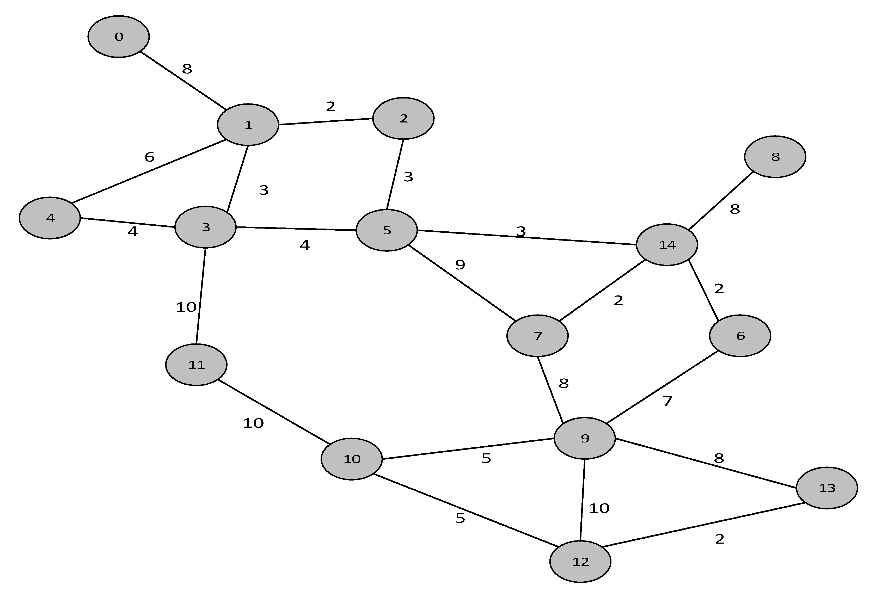
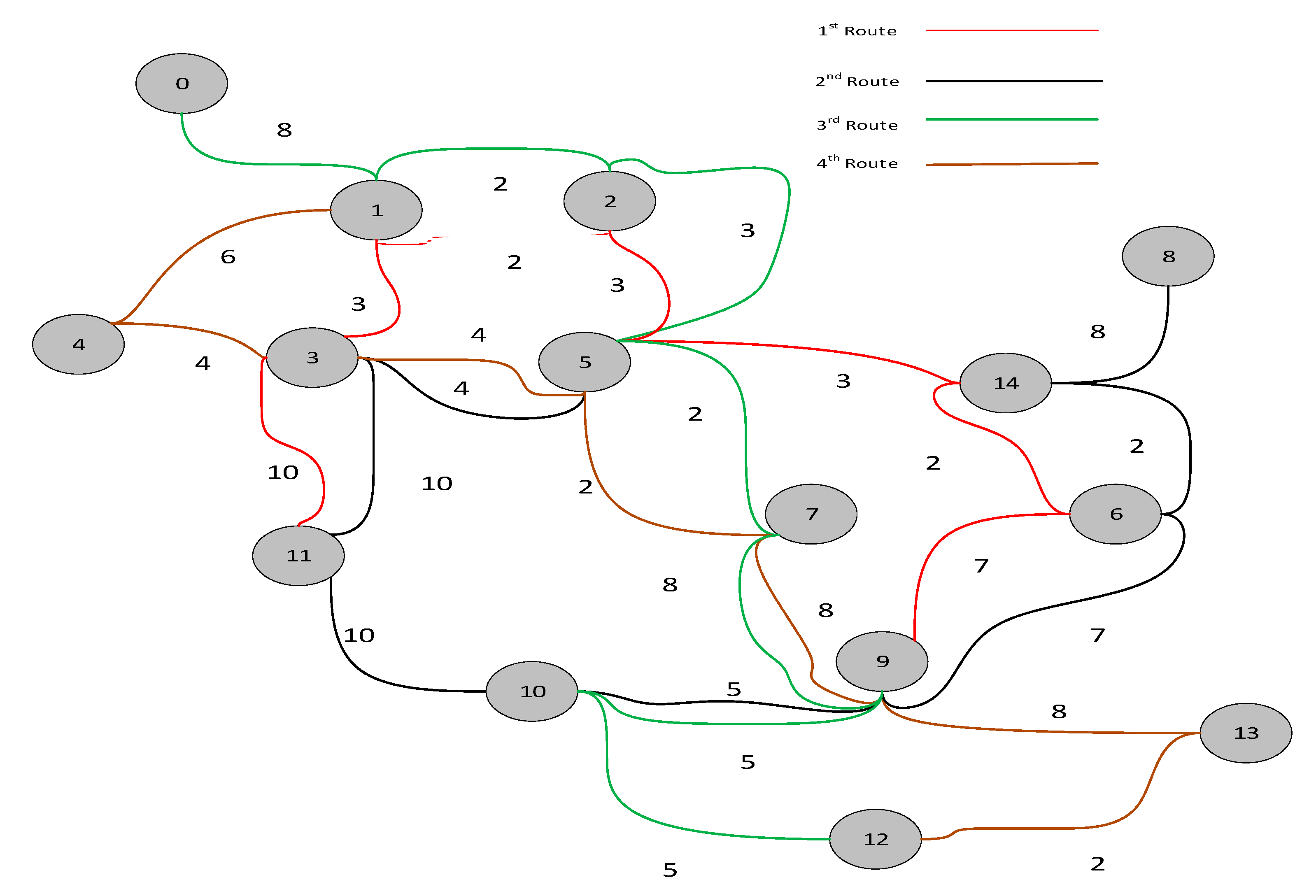
Τhe UTRP aims at developing a set of vehicle routes for an urban transit network while meeting all passengers’ and/or operator’s constraints. To model a transportation network, bus stops are modeled as adjacent nodes and, as a result, are linked by an edge. Several nodes connected by edges form a route. Several edges that connect nodes constitute a transportation path. In Figure 1, we present Mandl’s Swiss public transit network [25]. This network has fifteen nodes and twenty-one edges. Traveling times between nodes are defined by the numbers on the edges.
A candidate bus route (transportation path) constitutes several nodes connected by edges. We can define a valid bus route among nodes 8, 14 and 7 since these nodes are connected by existing edges of the network. However, nodes 9, 11 and 14 cannot form a bus route since there are not any existing edges that directly connect these nodes of the network. A route set is formed by one or more transportation paths (valid bus routes). Finally, all the routes of a route set that have been superimposed constitute the route network.
It is obvious that a route network should contain all nodes of the current transit network but may not include all its edges. As a matter of fact, we can say that each route network constitutes a subgraph of the existing road network (graph). An ideal route network, that is, a network satisfying all traveling demands, is a network with paths that connect each node of the network with every other node. To construct an efficient route network, we must acquire precise estimations of all travel demands. To realize these estimations, one should [44]:
- Undertake public and private vehicle analysis.
- Carry out surveys on the local population.
- Examine current ticket sales, etc.
However, these estimations are difficult to make, since travel demands are continuously modified and are very sensitive to factors like quality of service, pricing policy, etc. In the ideal case, the most travel demanding routes should be fulfilled with short travel paths and few vehicle transfers. In this way, however, the service level of all other routes will probably be affected. There are also several other factors that affect designing an effective route network, such as the local government’s transport management policies, the local area’s street environment, etc. [45].
2.2. Input Data and Optimization Criteria
The input instances that are used in current work are the Mandl’s Swiss transit network [25] and four transit networks that were contributed by Mumford [13]. The data used by the CSO-based algorithm as input are described in the following:
- Data that concern the connections among the network’s nodes (road network’s structure).
- Data that concern times needed to go from one node of the network to another (travel times).
- Data that concern travel demands between any two nodes of the road network (see Table 1 as an example).
The optimization criteria—in order of significance—on which the performance evaluation of the presented CSO algorithm is based, are described as follows ([13,14,26,31,36,38,43,46,47]):
- The percentage of unsatisfied demands (should be as low as possible, ideally equal to zero).
- The average travel time in minutes per transit user (should be as low as possible).
- The percentage of “with no transfers” satisfied demands (should be as high as possible).
Except for these three major criteria, there also some other constraints that should be fulfilled [47]:
- A minimum and a maximum number of nodes (length) must be defined for each route (defining that each route must have minimum and maximum length ensures route network’s connectivity and assists bus schedule adherence, respectively).
- In order passengers to be able to travel between any two nodes of the road network, there should be a path connecting any two of them (the road network should be a connected graph).
- Individual routes should not have any cycles or backtracks.
- To limit transportation cost, the service provider has usually predefined the number of routes in the route set.
The constraints mentioned above are considered as hard constraints that should never be violated by any acceptable solution, and are also considered by the presented CSO approach.
2.3. Solution Approaches and Drawbacks
As mentioned above, to design an effective route network, all criteria affecting its quality must be optimized. Consequently, one must formulate the mathematical model of the problem to include all these criteria so that its solution will result to an optimal set of routes for specific input data and under specific constraints. Researchers have attempted in the past to formulate and solve the UTRP problem using a mathematical approach ([26,48]). In these approaches, however, the desired characteristics of the route network are expressed as specific constraints, and the aim is to optimize a given function containing criteria affecting its quality [31]. Unfortunately, these attempts fail to define the specific routes of the network through the mathematical optimization problem. In [26], the authors conclude that UTRP is a difficult problem to represent using a mathematical approach due to the problem’s discrete nature. The basic variables of the problem are the nodes of the network and the edges that connect them. In [49], Newell stated that the UTRP, which is a non-convex optimization problem in its general form, is a difficult problem to solve. Consequently, there are some major UTRP features that increase its complexity. One of these features is its nonlinearity. Another one is that in many cases logical variables must be defined (e.g., to determine if two nodes are related to each other). Chakroborty claimed that conventional approaches find it difficult to solve the UTRP since they cannot represent it properly and effectively [31]. These methods often add extreme computational burden trying to represent it or even fail to depict it adequately. The UTRP is NP-complete in its general form concerning its computational complexity. This means that the difficulty to find a solution rises exponentially to its size, and there is no deterministic algorithm resulting in an acceptable solution in polynomial time.
3. The Proposed CSO-Based Algorithm
CSO-based algorithms imitate the collective behavior of non-distributed, self-organized physical systems. The capability of natural systems to demonstrate collective intelligent behavior is generally reported in publications as swarm intelligence [50]. These systems are usually composed of several autonomous agents: entities that are meant to execute different and specific operations. These agents interact locally either with each other or with their environment. Their interactions, although with no centralized control of behavior, often lead to a prospective collective one [51]. CSO algorithms were firstly proposed by Shu-Chuan et al. in 2006 [52] and have been successfully applied to other optimization problems, as presented in the related work section (see Section 1.1)
According to the classic CSO approach [50,52], there are two different states in which a cat can be during the optimization process: a) seeking mode and b) tracing mode. In seeking mode, each cat rests while examining its environment in order to decide which move should be its next one. In tracing mode, each cat moves rapidly hunting for food. The value of a Boolean variable determines whether a cat is in seeking mode or tracing mode. The way a cat is acting in seeking mode is affected by four parameters: (i) seeking memory pool (SMP), (ii) seeking range of the selected dimension (RSD), (iii) count of dimensions to change (CDC) and (iv) self-position consideration (SPC) [50,52]. The steps (in pseudocode) that each cat k (catk) is going to execute while in seeking mode are presented below:
- Step 1:
- Create j copies of the current position of catk (Note: j = SMP)If (the value of parameter SPC is true) j = (SMP − 1)Add the current position into the pool of candidate position to be moved to
- Step 2:
- For (each copy)Change the value of CDC dimensions at random (Note: these changes cannot exceed a percent ± RSD)
- Step 3:
- Calculate the fitness value for all candidate positions
- Step 4:
- If (the calculated finesses are not equal with each other)Calculate the probability Pi of selecting each candidate positionElsePi= 1.0, (Note: for all i)
- Step 5:
- Pick at random, among candidate positions, the position to which catk will be movedPlace catk to this positionProbability Pi, which is the probability of each candidate position to be selected for moving catkp there, is computed using Equation (1):where FSi is the fitness value of position i, FSmax is the biggest fitness value found, FSmin is the smallest fitness value found and FSb is equal to FSmax for maximization problems and equal to FSmin for minimization problems, respectively.
The steps (in pseudocode) that each cat k (catk) is going to execute while in tracing mode are presented below:
- Step 1:
- Update the velocity of each dimension of catk
- Step 2:
- If (the value of a velocity is outside allowed range)Set it equal to the maximum allowed value
- Step 3:
- Update the position of catk
The velocity of each dimension of catk is updated according to Equation (2):
where xbest,d is the position of the cat with the best fitness value up to that moment, xk,d is the position of catk, c1 is a constant affecting the change in the velocity of each dimension (most of the times set equal to 2.0 [50,52]) and r1 is a random value belonging to [0, 1]. The position of catk is updated according to Equation (3):
These two modes (seeking mode and tracing mode) are combined in the original CSO algorithm using a ratio determined by the parameter mixture ratio (MR) [50,52]. This parameter is usually set to a very small value favoring the seeking mode and thus reflecting the true behavior of cats, which spend most of their time—when awake—monitoring their environment instead of hunting for food. A more detailed description concerning the structure and operation of both modes is referenced in [50,52].
3.1. The Proposed CSO-Based Approach
3.1.1. Representation of Cats
A two-dimensional array is used for the representation of the route set. An analogous representation scheme was also adopted in [37]. If, for example, the route set consists of 5 routes, each one having a maximum of 9 nodes, we need an array of 5 × 9 = 45 cells to represent the solution. In Table 2, a random route set example of five routes, each one consisting of nine nodes at most, is presented. The 1st route begins at node 1, goes on to node 3, and then continues to node 4, etc. The other four routes are described in the same way. In the case of an empty cell, we put the value of “−1” in that cell, meaning that the respective route has been completed in a previous node. The 2nd route, for example, consists of seven nodes. As mentioned in previous sections, the total number of routes in the network as well as the maximum length of each route are both predefined by the transportation company and the local authorities, respectively.
3.1.2. Initialization of the Agents (Cats)
Since the UTRP is a very difficult problem to solve (see Section 2.3), we decided not to generate the initial population of route sets at random but to construct them based on some specific logical principles. Each route set is created by defining the number of routes it consists of. The initialization procedure, which has been adopted in this contribution, has been mainly based on the approach presented in [31] by Chakroborty and Wivedi, partly changed using the make-small-change procedure, as described by Fan and Mumford [37] and Fan et al. [15] and as it was also modified by Kechagiopoulos and Beligiannis [43]. In these approaches, an initial node set (INS) with K nodes is created, from which the first node is picked with a probability proportionate to its activity level. The value of parameter K, which is user defined, was chosen equal to 14 for the Mandl’s Swiss network, in line with the above works. Considering that Mandl’s network has 15 nodes, setting a value of 14 for the K parameter means that, besides node 14 which does not attract or generate any transfers (see Table 1), all other nodes are possible first nodes. For the four Mumford’s instances [13], all the nodes in each instance are considered as possible first nodes.
To maximize the number of nodes in each route, Kechagiopoulos and Beligiannis in [43] propose repetitive creation of a route 10 times to hold the one with the largest number of nodes. In the present approach, many original agents are created (limited by memory issues that are mainly affected by the size of the road network). Then, the initial whole population is filtered, and a smaller number of active agents remains (also limited by execution time issues). The filtering criterion is either the total number of nodes in the agent’s route set (we pick agents with as many as possible total number of nodes) or its fitness value (we pick agents with as bigger as possible fitness value). The first criterion has been used in trials focusing on customers’ interest, and the second criterion has been used in trials concerning the provider’s interest.
The initialization procedure satisfies the following demands:
- Establishment of a consistent route set.
- The duration of each route does not exceed the allowed limit.
- The minimum and maximum number of nodes on each route of the route set is within the predefined limits.
- There are no circles or inversions on each route in the route set.
The above requirements are ensured throughout the evolution of the algorithm. Initialization also determines the initial mode of each cat (if it is in tracing or in seeking mode) according to the mix ratio specified by the user (see Section 3.1.5).
3.1.3. Route Set Evaluation
Since the path of each route is strongly dependent on the paths of the other routes belonging to the same route set, separate evaluation of each route has no meaning. Consequently, all routes belonging to the same route set are evaluated together. The evaluation of route sets is based on several criteria measuring the “quality” level of each route set (see Section 2.2).
All criteria used for route set evaluation by the proposed CSO method are the ones already adopted by other researchers in the literature ([25,26,31,37,43,46]). To be more precise, we have adopted the evaluation procedure proposed in [31,37,43], where all evaluation criteria presented in Section 2.2 are put in a mathematical formula in order to calculate one single number, i.e., FIT(r). The arithmetic formula of FIT(r), which is used to calculate the fitness of each route set r, is the following equation:
where F1(r) is the score obtained by evaluating the route set r using the second criterion only (that is, the average travel time in minutes per transit user; see Section 2.2), F2(r) is the score obtained by evaluating the route set r using the third criterion (that is, the percentage of demand satisfied without any transfers, see Section 2.2) and F3(r) is the score obtained by evaluating the route set r using the first criterion only (that is, the percentage of demands unsatisfied; see Section 2.2). Parameters ω1, ω2, and ω3 are user specified weights for scores F1(r), F2(r) and F3(r), respectively. Based on the methodology introduced by Chakroborty and Wivedi [31], we estimate F1(r), F2(r) and F3(r).
F1(r) represents the average time spent by each passenger when using a specific route set. If the respective average traveling time is big, F1(r) has a small value; otherwise, its value is big. To estimate F1(r), one has both to calculate the average traveling time and determine whether the calculated value can be considered as “big” or “small”. Estimating F1(r) is performed according to the following steps:
1st Step: For every node pair (i,j) and a given route set r the in-vehicle travel time IVTi,j(r) is computed by determining the smallest time in which a passenger can travel from node i to node j using the routes of the rth transit route set. Traveling time Tp(r), on a path p, is calculated using the next mathematical formula:
where ta is the traveling time to node α starting from the previous node of the path, n is the number of transfers involved in path p and U is a time penalty paid for each transfer. In the current approach, parameter U is set to 5 min, as proposed in [25,26,31,37] and [43]. IVTi,j(r) is the smallest Tp(r) of all possible paths connecting nodes i and j.
2nd Step: The absolute minimum traveling time minTi,j between nodes i and j is calculated. This parameter is determined totally by the road network and neither by the route set nor the respective transfer delays.
3rd Step: Index fi,j(r) is determined by comparing traveling time minTi,j with the respective IVTi,j(r). Its value indicates whether IVTi,j(r) is “big” or “small”. Index fi,j(r) is estimated by the next mathematical formula:
where x = IVTi,j(r) − minTi,j, xm is the upper limit value of x, K1 is a positive user-defined parameter which defines the maximum value of fi,j(r) and K1/xm ≤ b1 ≤ 0. Index fi,j(r) is then used in order to calculate the value of F1(r) as follows:
where Sr is the set of node pairs (i,j) for which transfer demands, di,j, are satisfied by route set r.
One must notice that calculating the minimum time using Equation (7) is not so obvious, since different results may appear if someone considers transfer times or not. The selection of a route by a passenger may be done either without considering possible transfer delays (method A) or by considering all delays introduced by possible transfers (method B). We decided to examine both route evaluation methods and concluded that method B is much more computational demanding. Consequently, we used method A to evaluate routes during the execution of the algorithm and, then, the resulting route sets were also evaluated with method B, as it is obvious that this method is used in the published literature ([13,25,37]).
F2(r) represents the percentage of passengers traveling to their destination from their origin directly by making a single transfer or by making two transfers. Estimating F2(r) is realized by the next mathematical formula:
where K2 is a positive user-defined parameter which defines the upper limit of F2(r), K2/α ≤ b2 ≤ 2·K2/α and α is the upper limit of dΤ(r); dΤ(r) is estimated by the following formula:
where d0(r), d1(r), d2(r) are the percentages of passengers who travel from their origin to their destination directly, with one transfer or with two transfers, respectively. Parameters a, b and c are determined by the user (a ≥ b ≥ c). They represent the respective importance of the ways in which the demand should be satisfied in a qualitative route set, for example, trying to have a low percentage of intermediate transfers may lead to a larger average travel time.
dΤ(r) = a·d0(r) + b·d1(r) + c·d2(r)
F3(r) represents the percentage of passengers who are not able to go from their origin to their destination by route set r, and it is estimated as follows:
where K3 is a positive parameter determined by the user, defining the upper limit of F3(r); −K3 ≤ b3 ≤ 0; and dunsat(r) is the percentage of total transit demand which cannot be satisfied by route set r.
3.1.4. Calculating F4(r)—The Service Provider’s Cost Actor
Kechagiopoulos and Beligiannis [43] proposed the addition of a fourth cost, namely F4(r), in the evaluation function trying to construct qualitative route sets from the service provider’s scope. This fourth cost depends mainly on each route set’s total length. At first, they calculate the total length Ltot of each route set by summing all time distances between nodes belonging to the routes of each route set. Ltot is proportional to fuel consumption, a crucial factor for each service provider. The mathematical formula calculating score F4(r) is the following equation:
where Κ4 is a positive parameter determined by the user defining the upper limit of F4(r), −Κ4/x4m ≤ b4 ≤ 0 and x4m is a limit value for Ltot according to which route sets having Ltot values smaller than the value of x4m are supposed to be optimal. In these cases, F4(r) reaches its maximum value.
3.1.5. Constructing the Best Route Procedure
The algorithm starts by reading the input data, i.e.,:
- Data concerning the road network as well as the transfer requests.
- Data concerning problem requirements (number of routes in the resulting route set, maximum number of nodes for each route, the maximum time length per route and the minimum nodes per rout).
- Transfer penalty.
- Test’s seed.
From the initialization phase, each cat acquires a property that determines its initial mode in terms of seeking mode or tracing mode. A small percentage of cats is put into seeking mode and the rest in tracing mode. This percentage is determined by the value of the mixture ratio (MR) parameter, which in this contribution was set to 0.04 (see Section 3.1.8 and Table 3). MR determines the proportion of cats in seeking mode in the total active cats’ population [52]. An MR value equal to 0.04 means that about 4% of the population is in seeking mode.
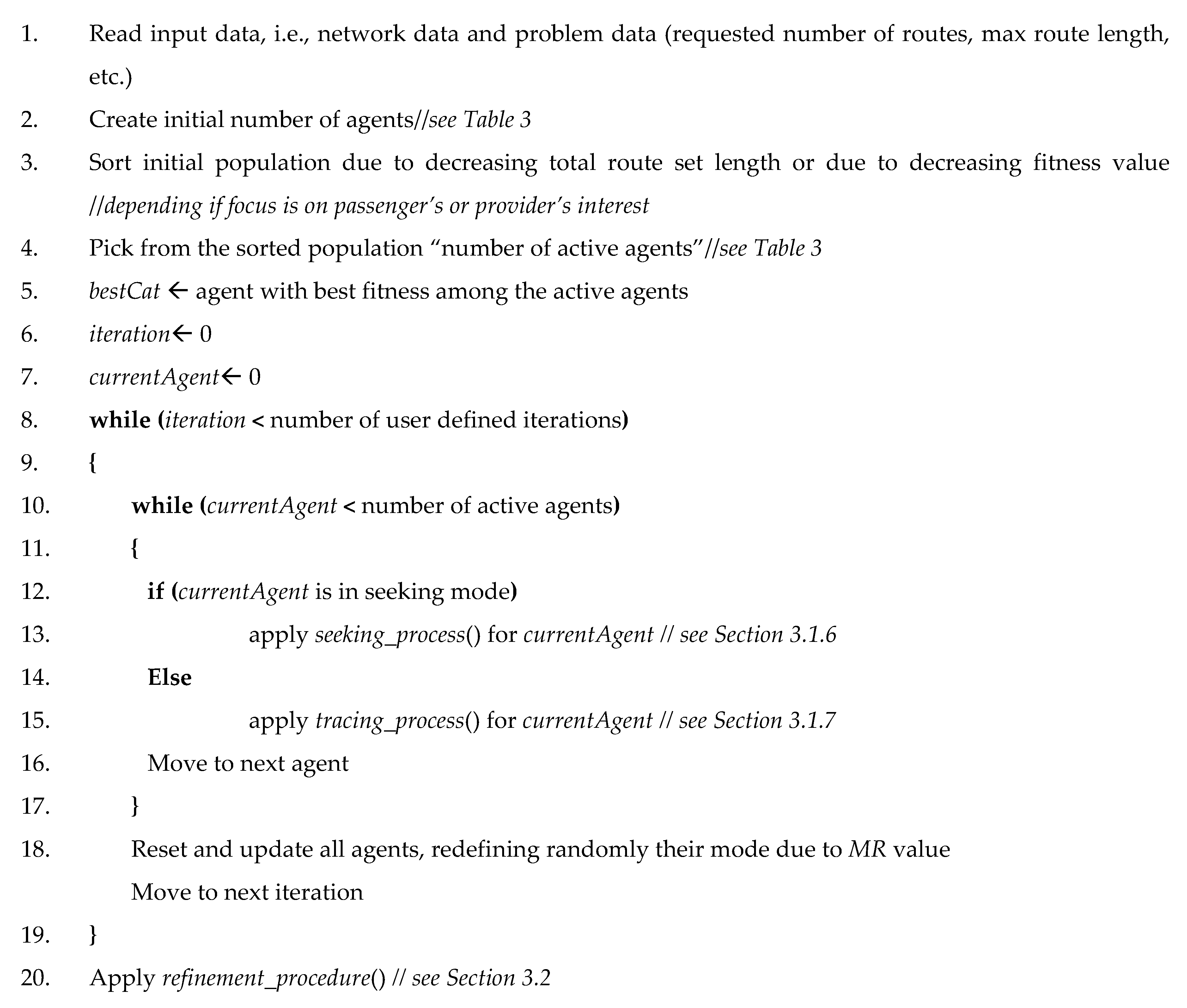
The main phase of the route set configuration algorithm runs for a predetermined number of iterations (see Section 3.1.8 and Table 3). It consists essentially in separating the active cats according to the mode they are in (seeking mode or tracing mode) and applying to them the corresponding seeking mode procedure (see Section 3.1.6) or tracing mode procedure (see Section 3.1.7). After completing these procedures, each cat’s mode is redefined, and the process is repeated. When the predetermined number of iterations is completed, the algorithm ends its main phase and enters an improvement phase of the resulting solution. In this phase, a refinement procedure which seeks to improve the resulting solution by adding one node at the end of each route of the final route set is applied (see Section 3.2). The pseudocode in Figure 2 demonstrates the structure of the proposed algorithm. Steps 1–4 constitute the initialization phase; steps 5–19 comprise the main phase of the algorithm, while step 20 concerns the execution of the refinement procedure.
3.1.6. Seeking Mode Process
The seeking process intends to bring about changes to the cats that are in seeking mode in order to improve the global solution. In the seeking process, a random route is selected from the best agent (i.e., the best route set so far) and takes the place of the corresponding route of the cat to which the process is applied. If none of the hard constraints is violated and the cat’s fitness improves, the substitution is finalized. Otherwise, the cat returns to its original state. If, in addition, replacement leads to better fitness than the existing bestFitness, then the bestCat is also updated and substituted by current cat in which seeking process is applied (Figure 3).
3.1.7. Tracing Mode Process
The tracing process seeks to make changes locally, slightly altering the structure of the cats in tracing mode. This increases the chance of improving the route sets represented by cats. The changes are probabilistic rather than deterministic. Thus, both the diversity of the population and its dispersion in as much of the solution space as possible are maintained. During the tracing process, several copies of the cat to which the tracing process is applied are created. This number of copies is equal to the seeking memory pool (SMP) size parameter [52], which in the current implementation is set to 10 (see Section 3.1.8 and Table 3). For each copy of these, a random route is selected from the route set that cat represents, and a random location on that route is marked which is not empty (i.e., has value not equal to −1). All the road network nodes are overlooked, and the first one that can replace the node in the chosen location is selected. If the route set consistency is not violated, the maximum allowed length of the selected route is not exceeded and no circles or inversions are created, the substitution is finalized. Otherwise, the process proceeds to the next road network node. The process for the current copy is completed when there is a successful replacement or when the road network nodes are exhausted. The above procedure is repeated for all copies of the SMP. The fitness value of each copy is then calculated, and if all fitness values are the same, the probability of choosing each copy is set to 1. Otherwise, the probability of choosing each copy is calculated according to the value of the ratio , where Fitnessmin and Fitnessmax are respectively the minimum and maximum fitness values among all copies of cat, and Fitnesscopy is the fitness value of the current copy. The process is completed by selecting a copy replacing the cat to which the tracing process is applied, with a probability of selection equal to the one previously calculated (Figure 4).
3.1.8. Setting the Algorithm’s Parameters Values
Most parameters’ values used by the algorithm (presented in Table 3) are determined based on efficiency requirements, constraints of computational resources and the respective literature [18,50,51,52]. The determination of the rest parameters’ values was conducted after exhaustive experiments (by trial and error), and the selected values where the ones that utilize the algorithm’s performance. These parameters are the following:
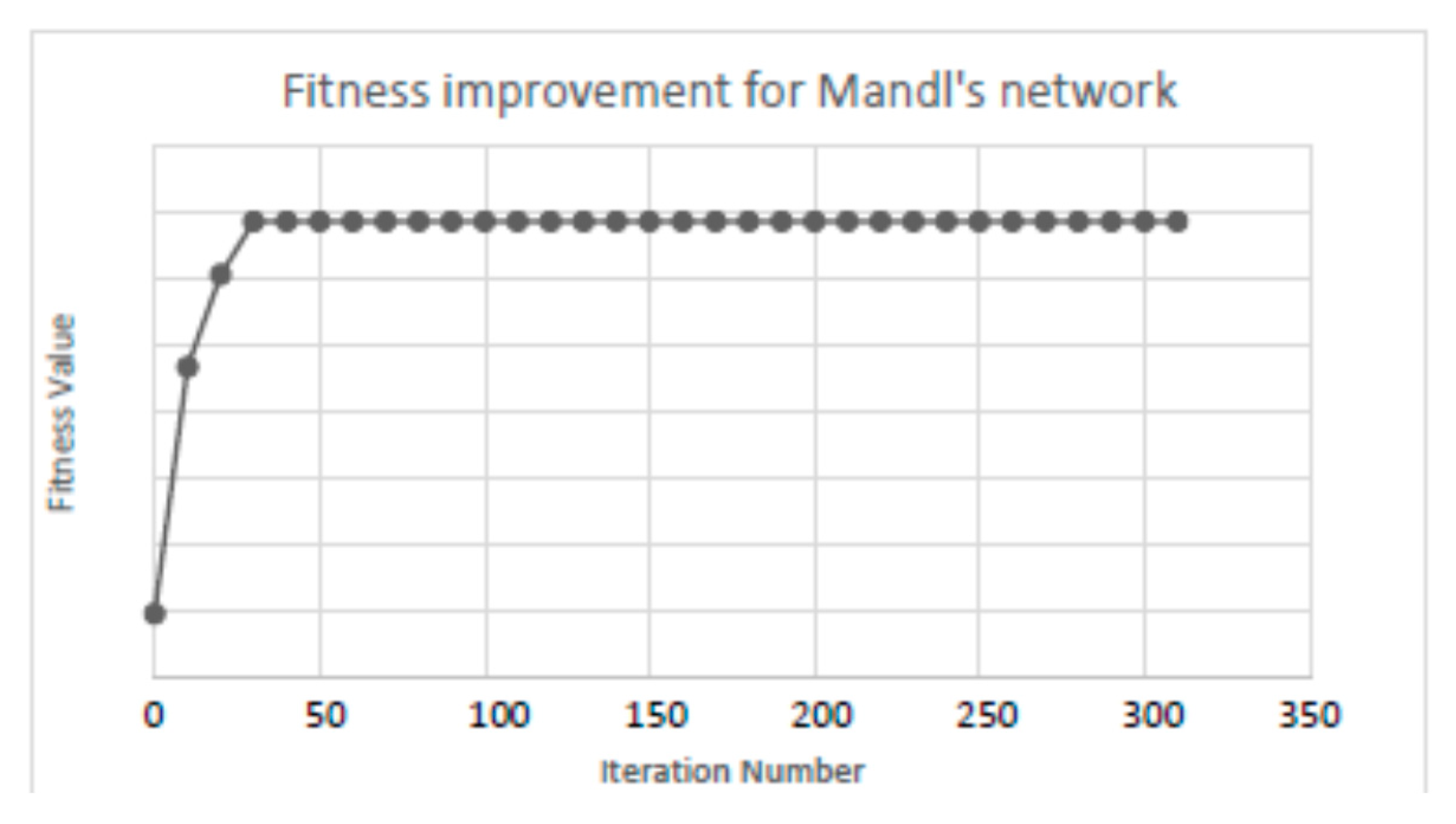
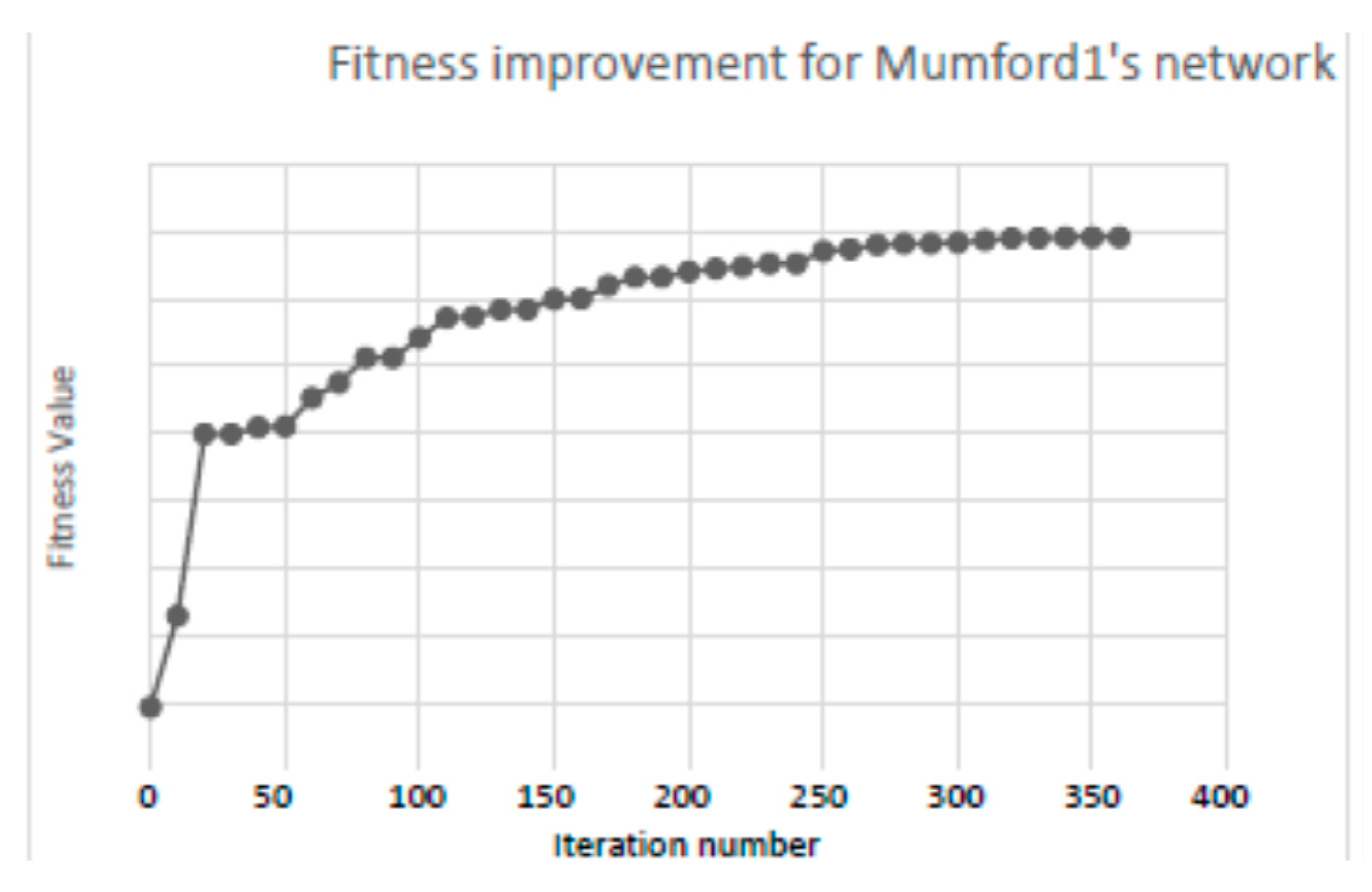
Number of iterations: The number of iterations is determined mainly by constraints related to the execution time of the algorithm. Because the size of the solution space is increasing as the size of the road network increases (see Figure 5 and Figure 6 for example), the number of generations depends on the size of the network and is fixed to 300 + number of nodes of the network, since we noticed that after 300 iterations the improvement in the algorithm’s performance, for the tested networks, is insignificant.
Initial number of agents (cats): The number of agents originally created, from which the most robust are selected, is mainly determined by constraints on computing resources (memory). For relatively small networks, this number can be set to a bigger value, and for larger networks, a smaller value should be selected. After many experiments, this number has values from 135 to 1000.
Number of active agents (cats): The number of active agents used throughout the execution of the algorithm is mainly determined by the requirement that the algorithm completion time must be limited to acceptable frames. For relatively small networks. this number can be set to a bigger value, and for larger networks, a smaller value should be selected. After many experiments, this number has values from 50 to 500.
Coefficients ω1, ω2, ω3: By adjusting the values of ω1, ω2and ω3, we can control the effect of the terms F1, F2 and F3 on the fitness value (see Section 3.1.3 and Equation (1)). When performing the experimental tests, it was observed that when the number of routes in the route set is small, solutions can be found in which there is a non-zero percentage of unsatisfactory transfer demands. After exhaustive testing, we decided to set the values of ω1 and ω2 to 1.0. It was also observed that in some cases, the algorithm produced infeasible solutions when the number of routes was limited to four. Therefore, the ω3 value was set at 121.0 when the algorithm had to deal with the four routes case. Alternatively, one could adjust the value of the K3 factor accordingly.
3.2. The Refinement Procedure
The algorithm has been enriched with a solution improvement process that is activated after the end of the main phase of the algorithm. This process seeks to improve the solution by adding one node at the end of each route of the final route set. There is a pre-refinement phase in which all routes of the route set are identified if they can be refined. A route can be improved (i.e., refined) when the number of nodes in the route is less than the maximum number of nodes per route. We check whether a node could be added after the last node of the route without a circle being created or violating the connectivity of the route set. If this is the case, then the route is considered a route that can be refined. If not, the route is reversed, and the same pre-refinement procedure is repeated once more. The refinement procedure is not applied in the case in which we are focusing on provider’s interest (see Section 4.3).
The refinement procedure is described in Figure 7. Steps 1–12 constitute the pre-refinement phase, while steps 13–29 comprise the main refinement phase.
4. Computational Results
To evaluate the performance of the algorithm, five input files from the international bibliography containing five road networks data were used: the file of Mandl’s road network [25] and four files introduced by Mumford [13], namely Mumford0, Mumford1, Mumford2 and Mumford3. Table 4 contains the attributes of these files.
Evaluation and comparison of route sets is made considering the following criteria (in order of significance):
- Unsatisfied travel requirements (dunsatt), which should be as small as possible and ideally 0%.
- Average travelling time per user (att), which should be as small as possible and is equal to , where 0≤ i ≤ number of nodes, 0≤ j ≤ number of nodes, dij represents the transferring demands and tij symbolizes the travelling time between node i and node j, respectively, using the route set which is under evaluation (transferring delays are included). Note that this is different from Equation (4), in which we consider only the travelling demands that are satisfied by the route set, i.e., travelling demands that are satisfied with less than three transfers. Alternatively, we use the total user cost (ttc in minutes [40,42]) which also should be as small as possible.
- Percentage of travels with zero transfers (d0), which should be as large as possible and ideally 100%.
Code was created in Java, using the Eclipse IDE. All tests were performed in a Windows Vista Home Premium (SP2) 32-bit OS machine, with an Intel Core 2 CPU, T7200 @2.00 GHz and 2.00 GB RAM.
All five instances have been evaluated using the same method. If there are any discrepancies between the published results and our evaluation, both results are published (this is the case for Mumford [13] solutions). Details about how to run the proposed CSO algorithm, the input files used, the output files containing the best results achieved, as well as, the executable program of the proposed CSO algorithm are available online at [53], so as to be easy for the interested reader to reproduce the below-mentioned results.
4.1. Applying CSO to Mandl’s Network Instance
There were executed 100 repeatable Monte Carlo runs per instance per required number of routes. In Table 5, Table 6, Table 7, Table 8, Table 9, Table 10, Table 11 and Table 12, the best and worst results achieved by the proposed CSO algorithm are selected based on the three criteria presented in the former paragraphs using the proposed order of significance. Moreover, the average and standard deviation values presented are the ones calculated over all 100 repeatable Monte Carlo runs. In bold are the values which determine which of the proposed approaches achieve the best results.
The best solution (route set) with four routes found by the proposed CSO algorithm, which is presented in Figure 8, is the following:
- 1st Route: {9 6 14 5 2 1 3 11}
- Route: {5 3 11 10 9 6 14 8}
- Route: {0 1 2 5 7 9 10 12}
- Route: {12 13 9 7 5 3 4 1}
As Table 5 shows, the route set that the CSO approach produced for a four-route route set is the second best achieved solution among other approaches. Even the worst achieved solution by the CSO algorithm is better than many of the best solutions achieved by other approaches. The route set that CSO produces has an average travelling time per user that differs by only 5.34% from the ideal one (see Table 4).
The best solution (route set) with six routes found by the proposed CSO algorithm is the following:
- 1st Route: {0 1 2 5 14 6 9 13}
- Route: {0 1 4 3 5 7 9 10}
- Route: {0 1 2 5 7 9 10 12}
- Route: {0 1 3 11 10 12 13 9}
- Route: {4 3 11 10 9 6 14 8}
- Route: {6 14 7 5 3 11 10 12}
As Table 6 shows, the route set that the CSO approach produced for a six-route route set improves the best achieved solution ([38]) to 0.06% (same average travelling time; better zero transfers’ satisfied transfer demands). Even the worst achieved solution by the CSO algorithm is better than many of the best solutions achieved by other approaches, and all transfer demands are satisfied with no more than one transfer. The route set that CSO produced gives an average travelling time per user that differs by 2.14% from the ideal one (see Table 4).
The best solution (route set) with routes found by the proposed CSO algorithm is the following:
- 1st Route: {0 1 2 5 7 9 10 12}
- Route: {7 9 6 14 5 2 1 0}
- Route: {6 14 7 5 3 1 2 −1}
- Route: {0 1 4 3 5 7 9 10}
- Route: {5 3 11 10 9 6 14 8}
- Route: {8 14 5 2 1 4 3 11}
- Route: {0 1 3 11 10 12 13 9}
As Table 7 shows, the route set that the CSO approach produced for a seven-route route set improves the best achieved solution ([23]) to 0.3% (10.12 min per user from 10.15 min per user). Even the worst achieved solution by the CSO algorithm is better than many of the best solutions achieved by other approaches. All transfer demands are satisfied with no more than one transfer in both best and worst solutions. The route set that CSO produced gives an average travelling time per user that differs by 1.14% from the ideal one (see Table 4).
The best route set with eight routes created using the proposed CSO algorithm:
- 1st Route: {0 1 4 3 5 7 9 10}
- Route: {0 1 2 5 14 6 9 13}
- Route: {0 1 2 5 7 9 10 12}
- Route: {6 14 5 3 4 1 2 −1}
- Route: {9 10 11 3 5 7 14 6}
- Route: {9 13 12 10 11 3 1 0}
- Route: {4 3 11 10 9 6 14 8}
- Route: {8 14 5 2 1 3 11 −1}
As Table 8 shows, the route set that the CSO approach produced for an eight-route route set improves the best achieved solution ([45]) to 0.1% for the average travelling time. Even the worst achieved solution by the CSO algorithm is better than all but one of the best solutions achieved by other approaches. All transfer demands are satisfied with no more than one transfer in both best and worst solutions. The route set that CSO produced gives an average travelling time per user that differs by 0.74% from the ideal one (see Table 4).
In Muhammed et al. [38] and Nikolic and Teodorovic [40], the maximum number of nodes for each route was limited to 13 and 11, respectively. For a fair comparison, we ran tests using CSO, using the same maximum number of nodes per route. In Table 9, Table 10, Table 11 and Table 12, the comparative best results are presented. In bold are the values which determine which of the proposed approaches achieve the best results.
4.2. Applying CSO to Mumford’s Instances
There were 100 Monte Carlo trials executed per instance per required number of routes. In Table 13, Table 14, Table 15 and Table 16, the best results achieved by the proposed CSO algorithm are presented based on the three criteria presented at the beginning of Section 4 using the proposed order of significance. In bold are the values which determine which of the proposed approaches achieve the best results.
4.3. Considering the Provider’s Operational Cost
The provider’s operational cost is considered in this section by investigating to what extent the total length of all routes affects it. Of course, the smaller the total length of all routes, the bigger the profit for transport companies. As mentioned (see Section 1), Kechagiopoulos and Beligiannis [43] proposed a method of balancing costs between the customer and the provider, admitting a fourth term F4(r) in the evaluation function (Equation (8)). In this contribution, we adopt the same method using the same values for the coefficients for calculating the term F4(r) (see Table 3). Score F4(r) is summed in an analogous way to the rest of the Fi scores (). The ω4 weight is set equal to 1. As seen in Section 3.1.3, the Ki values are the maximum values that the respective Fi scores can obtain. Thus, we can modify Ki values to put analogous emphasis on a specific score. We can reach the same goal by changing the values of weights ωi too.
When considering score F4(r), one can clearly realize the multi-objective nature of the applied algorithm. As mentioned above, score F4(r) is mainly affected by the total length of the entire route set, which clearly affects operational costs, for example, average fuel consumption, and introduces in the evaluation function the service provider’s point of view. Since the value of F4(r) increases as the total route set length decreases,F4(r) is competing with the other Fi scores. Computational experiments show that if the algorithm’s parameter values are properly chosen, the algorithm can succeed in constructing route sets that balance the conflicting goals (passenger’s demands vs. operational costs). In order to obtain optimal results from the passengers’ scope and be able to have a fair comparison of the algorithm’s performance with other methods reported in the literature, the weight value of F4(r) was set to 0 (operational cost not taken into account) in all experimental results presented in Section 4.1 and Section 4.2.
In Table 17 and Table 18, the evaluation and comparison of route sets constructed by the proposed CSO algorithm and the approach by Kechagiopoulos and Beligiannis [43] is made considering the following criteria (in order of significance):
- Total length (Ltot) in minutes of each route set, which should be as small as possible.
- Unsatisfied travel requirements (dunsatt), which should be as small as possible and ideally 0%.
- Average travelling time per user (att), which should be as small as possible.
- Percentage of travels with zero transfers (d0), which should be as large as possible and ideally 100%.
Note that in this case, the agents that remain active during the execution of the algorithm were initially picked according to their fitness value (see Section 3.2), and the refinement phase (see Section 3.2) is not activated.
In the first set of experiments, parameter K4 was set to 10, while x4m varies from 20 to 200 min. In Table 17, we present the average values of all evaluation criteria. Both algorithms were executed for 100 Monte Carlo runs, the number of routes equals 4, and the maximum number of nodes is restricted to 8.
As can be seen from Table 17, the approach of the CSO algorithm produces in all cases better results according to the criteria set forth above. The cost for the transmission system provider is about 72.9% on average when compared to the corresponding costs generated by the approach of [43]. The volatility of Ltot values is much smaller than the corresponding volatility displayed at [43]. This means that we could set x4m to a value bigger than 160 and produce a route set with a cost for the provider equal to 75.45 on average. At the same time, we achieve route sets that meet the requirements of passengers with no more than two transfers. The time burden for passengers in this case reaches 10.3% on average when compared to [43].
In the second set of experiments, parameter K4 was set to 10, while x4m varies from 80 to 160 min. In Table 18, we present the average values of all evaluation criteria. Both algorithms were executed for 100 Monte Carlo runs, the number of routes equals 4, and the maximum number of nodes is restricted to 10.
As can be seen from Table 18, the approach of the CSO algorithm produces in all cases better results according to the criteria set forth above. The cost for the transmission system provider is about 65.6% on average compared to the corresponding costs generated by the approach of [43]. The volatility of Ltot values is much smaller than the corresponding volatility displayed at [43]. This means that we could set x4m to a value equal to 160 and produce a route set with a cost for the provider equal to 75.9 on average. The time burden for passengers in this case reaches 20.9% on average when compared to [43].
In conclusion, we can adjust algorithm’s parameters to fulfill passengers demands and, at the same time, succeed in decreasing operational costs. However, designing route sets with very small route lengths should be avoided, since very small route lengths demand higher frequency of bus schedules, which is not acceptable in general.
5. Conclusions—Future Work
In this work, a robust CSO-based algorithm has been constructed and applied to the urban transit routing problem (UTRP). Efficient and feasible near-optimal route networks for public transit networks were designed using this novel approach. To our knowledge, this is the first time that a CSO-based algorithm is applied to solve the UTRP. Five input instances were used as benchmark problems, derived from international literature, which consist of well-known test instances for the UTRP in the respective literature. Experimental results showed that the proposed CSO-based algorithm achieves in all test instances very satisfactory results comparable with the best results found to date by other effective published approaches applied to the same test instances using the same evaluation criteria. This fact demonstrates that applying CSO-based algorithms is a very good choice to effectively solve the UTRP, excluding the fact that the proposed algorithm also considers the optimization of the provider’s operational cost. Some experimental results show that by adjusting the algorithm’s parameters, the proposed algorithm can both fulfill passengers’ demands and, at the same time, succeed in decreasing operational costs. A weak spot of the proposed algorithm is the determination of parameters’ values, which plays a significant role in the algorithm’s optimization capability. A more systematic method to determine the (near) optimal values of all algorithms’ parameters will be one of the main issues of our future work. Moreover, further research toward optimizing the cost of the service provider as well as applying the algorithm to relevant vehicle routing problems, such as the capacitated vehicle routing problem (CVRP) and the open vehicle routing problem, are future goals of the authors.
Author Contributions
Formal analysis, investigation, resources, software, validation, visualization, writing—original draft, I.V.K.; methodology, validation, visualization, writing—review & editing, I.X.T.; conceptualization, methodology, project administration, supervision, writing—review & editing, G.N.B. All authors have read and agreed to the published version of the manuscript.
Funding
This research received no external funding.
Conflicts of Interest
The authors declare no conflict of interest.
References
- White, P. Public Transport: Its Planning, Management and Operation, 4th ed.; Spon Press: London, UK, 2002. [Google Scholar]
- Farahani, R.Z.; Miandoabchi, E.; Szeto, W.Y.; Rashidi, H. A review of urban transportation network design problems. Eur. J. Oper. Res. 2013, 229, 281–302. [Google Scholar] [CrossRef] [Green Version]
- Mackett, R.L.; Edwards, M. The impact of new urban public transport systems: Will the expectations be met? Transp. Res. A Policy Pract. 1998, 32, 231–245. [Google Scholar] [CrossRef]
- Zeng, Q.F.; Mouskos, K.C. Heuristic Search Strategies to Solve Transportation Network Design Problems; Final Report; Department of Transportation: Trenton, New Jersey, USA, 1997.
- Stephen, S.; Liu, Z. China’s urban Transport Development Strategy. In Proceedings of the Symposium, Beijing, China, 8–10 November 1995. [Google Scholar]
- Balchin, P.N.; Bull, G.H.; Kieve, J.L. Urban Land Economics and Public Policy, 5th ed.; Palgrave Macmillan: London, UK, 1995. [Google Scholar]
- Criden, M. The Stranded Poor: Recognizing the Importance of Public Transportation for Low-Income Households; National Association for State Community Service Programs: Washington, DC, USA, 2008.
- Edwards, M.; Mackett, R.L. Developing new urban public transport systems: An irrational decision-making process. Transp. Policy 1996, 3, 225–239. [Google Scholar] [CrossRef]
- Chester, M.; Pincetl, S.; Elizabeth, Z.; Eisenstein, W.; Matute, J. Infrastructure and automobile shifts: Positioning transit to reduce life-cycle environmental impacts for urban sustainability goals. Environ. Res. Lett. 1996, 8, 015041. [Google Scholar] [CrossRef]
- INRO>Emme Transportation Forecasting Software. Available online: http://www.inrosoftware.com/en/products/emme/index.php (accessed on 23 July 2020).
- ATKINS–SATURN. Available online: http://www.saturnsoftware.co.uk/index.html (accessed on 23 July 2020).
- Vision Traffic—PTV Group. Available online: http://www.ptv-vision.com/en-uk/products/visiontraffic-suite/ptv-visum/overview/ (accessed on 23 July 2020).
- Mumford, C.L. New Heuristic and Evolutionary Operators for the Multi-Objective Urban Transit Routing Problem. In Proceedings of the IEEE Congress on Evolutionary Computation (CEC ′13), Cancun, Mexico, 20–23 June 2013; pp. 939–946. [Google Scholar]
- Yang, Z.; Yu, B.; Cheng, C. A parallel ant colony algorithm for bus network optimization. Comput.-Aided Civil Infrastruct. Eng. 2007, 22, 44–55. [Google Scholar] [CrossRef]
- Fan, L.; Mumford, C.L.; Evans, D. A Simple Multi-Objective Optimization Algorithm for the Urban Transit Routing Problem. In Proceedings of the IEEE Congress on Evolutionary Computation (CEC ′09), Trondheim, Norway, 18–21 May 2009; pp. 1–7. [Google Scholar]
- Zhang, J.; Lu, H.; Fan, L. The Multi-Objective Optimization Algorithm to a Simple Model of Urban Transit Routing Problem. In Proceedings of the Sixth International Conference on Natural Computation (ICNC ′10), Yantai, China, 10–12 August 2010; pp. 2812–2815. [Google Scholar]
- Chew, O.C.; Lee, L.S. A genetic algorithm for urban transit routing problem. Int. J. Mod. Phys. 2012, 9, 411–421. [Google Scholar] [CrossRef] [Green Version]
- Skoullis, V.I.; Tassopoulos, I.X.; Beligiannis, G.N. Solving the high school timetabling problem using a hybrid cat swarm optimization based algorithm. Appl. Soft Comput. 2017, 52, 277–289. [Google Scholar] [CrossRef]
- Bhopender, K.; Mala, K.; Poonam, S. Discrete Binary Cat Swarm Optimization for Scheduling Workflow Applications in Cloud Systems. In Proceedings of the 3rd International Conference on Computational Intelligence & Communication Technology (CICT ’17), Ghaziabad, India, 9–10 February 2017; pp. 1–6. [Google Scholar]
- Pei-Wei, T.; Lingping, K.; Snasel, V.; Jeng-Shyang, P.; Vaci, I.; Zhi-Yong, H. Utilizing Cat Swarm Optimization in Allocating the Sink Node in the Wireless Sensor Network Environment. In Proceedings of the 3rd International Conference on Computing Measurement Control and Sensor Network (CMCSN ‘16), Matsue, Japan, 20–22 May 2016; pp. 166–169. [Google Scholar]
- Razzaq, S.; Maqbool, F.; Hussain, A. Modified Cat Swarm Optimization for Clustering. In Advances in Brain Inspired Cognitive Systems; Liu, C., Hussain, A., Luo, B., Tan, K., Zeng, Y., Zhang, Z., Eds.; Springer: Cham, Switzerland, 2016; Volume 10023, pp. 161–170. [Google Scholar]
- Broderick, C.; Soto, R.; Berríos, N.; Johnson, F.; Paredes, F. Solving the Set Covering Problem with Binary Cat Swarm Optimization. In Advances in Swarm and Computational Intelligence; Tan, Y., Shi, Y., Buarque, F., Gelbukh, A., Das, S., Engelbrecht, A., Eds.; Springer: Cham, Switzerland, 2015; Volume 9140, pp. 41–48. [Google Scholar]
- Bouzidi, A.; Riffi, E.M.; Barkatou, M. Cat swarm optimization for solving the open shop scheduling problem. Int. J. Ind. Eng. 2019, 15, 367–378. [Google Scholar] [CrossRef] [Green Version]
- Kencana, E.N.; Kiswanti, N.; Sari, K. The application of cat swarm optimization in classifying small loan performance. J. Phys. Conf. Ser. 2017, 893, 012037. [Google Scholar] [CrossRef]
- Mandl, C.E. Applied Network Optimization; Academic Press: London, UK, 1979. [Google Scholar]
- Baaj, M.H.; Mahmassani, H.S. An AI-based approach for transit route system planning and design. J. Adv. Transp. 1991, 25, 187–209. [Google Scholar] [CrossRef]
- Buda, A.T.; Lee, L.S. Differential evolution for urban transit routing problem. J. Comput. Chem. 2016, 4, 11–25. [Google Scholar]
- Owais, M.; Osman, M.K. Complete hierarchical multi-objective genetic algorithm for transit network design problem. Expert Syst. Appl. 2018, 114, 143–154. [Google Scholar] [CrossRef]
- Buda, A.T.; Lee, L.S. Hybrid differential evolution-particle swarm optimization for multiobjective urban transit network design problem with homogeneous buses. Math. Probl. Eng. 2019, 2019, 5963240. [Google Scholar]
- Nayeem, M.A.; Islam, M.M.; Yao, X. Solving transport network design problem using many-objective evolutionary approach. IEEE Trans. Intell. Transp. Syst. 2019, 20, 3952–3963. [Google Scholar] [CrossRef]
- Chakroborty, P.; Wivedi, T. Optimal Route Network Design for transit systems using genetic algorithms. Eng. Optimiz. 2002, 34, 83–100. [Google Scholar] [CrossRef]
- Jha, S.B.; Jha, J.; Tiwari, M. A multi-objective meta-heuristic approach for transit network design and frequency setting problem in a bus transit system. Comput. Ind. Eng. 2019, 130, 166–186. [Google Scholar] [CrossRef]
- Iliopoulou, C.; Kepaptsoglou, K.; Vlachogianni, E.I. Metaheuristics for the transit route network design problem: A review and comparative analysis. Public Transp. 2019, 11, 487–521. [Google Scholar] [CrossRef]
- Kim, M.; Kho, S.-Y.; Kim, D.-K. A transit route network design problem considering equity. Sustainability 2019, 11, 3527. [Google Scholar] [CrossRef] [Green Version]
- Iliopoulou, C.; Tassopoulos, I.; Kepaptsoglou, K.; Beligiannis, G. Electric transit route network design problem: Model and application. Transp. Res. Record 2019, 2673, 264–274. [Google Scholar] [CrossRef]
- Kidwai, F.A. Optimal Design of Bus Transit Network: A Genetic Algorithm Based Approach. Ph.D. Thesis, Department of Civil Engineering, Indian Institute of Technology, Kanpur, India, 1998. [Google Scholar]
- Fan, L.; Mumford, C.L. A metaheuristic approach to the urban transit routing problem. J. Heuristics 2010, 16, 353–372. [Google Scholar] [CrossRef]
- Nayeem, M.A.; Rahman, M.K.; Rahman, M.S. Transit network design by genetic algorithm with elitism. Transp. Res. Part C 2014, 46, 30–45. [Google Scholar] [CrossRef]
- Kilic, F.; Gok, M. A demand based route generation algorithm for public transit network design. Comput. Oper. Res. 2014, 51, 21–29. [Google Scholar] [CrossRef]
- Nikolic, M.; Teodorovic, D. A simultaneous transit network design and frequency setting: Computing with bees. Expert Syst. Appl. 2014, 41, 7200–7209. [Google Scholar] [CrossRef]
- Nikolic, M.; Teodorovic, D. Transit network design by Bee Colony Optimization. Expert Syst. Appl. 2013, 40, 5945–5955. [Google Scholar] [CrossRef]
- Zhao, H.; Jiang, R. The Memetic algorithm for the optimization of urban transit network. Expert Syst. Appl. 2015, 42, 3760–3773. [Google Scholar] [CrossRef]
- Kechagiopoulos, P.N.; Beligiannis, G.N. Solving the Urban Transit Routing Problem using a particle swarm optimization based algorithm. Appl. Soft Comput. 2014, 21, 654–676. [Google Scholar] [CrossRef]
- Balcombe, R. The Demand for Public Transport: A Practical Guide; Transportation Research Laboratory: London, UK, 2004. [Google Scholar]
- Emerson, B. Design and Planning Guidelines for Public Transport Infrastructure: Bus Route Planning and Transit Streets; Public Transport Authority: Washingtion, DC, USA, 2003.
- Mandl, C.E. Evaluation and optimization of urban public transport networks. Eur. J. Oper. Res. 1980, 5, 396–404. [Google Scholar] [CrossRef]
- Zhao, F.; Gan, A. Optimization of Transit Network to Minimize Transfers; Final Report; Florida Department of Transportation: Tallahassee, FL, USA, 2003.
- Israeli, Y.; Ceder, A. Designing Transit Routes at the Network Level. In Proceedings of the IEEE Vehicle Navigation and Information Systems Conference (VNIS’89), Toronto, ON, Canada, 11–13 September 1989; pp. 310–316. [Google Scholar]
- Newell, G.F. Some issues relating to the optimal design of bus routes. Transp. Sci. 1979, 13, 20–35. [Google Scholar] [CrossRef]
- Shu-Chuan, C.; Pei-Wei, T.; Pan, J.S. Cat Swarm Optimization. In Proceedings of the 9th Pacific Rim International Conference on Artificial Intelligence; Yang, Q., Webb, G., Eds.; Springer: Berlin/Heidelberg, Germany, 2006; Volume 4099, pp. 1513–1523. [Google Scholar]
- Fister, J.; Yang, X.-S.; Fister, I.; Brest, J.; Fister, D. A Brief Review of Nature-Inspired Algorithms for Optimization. Elektron. Vestn. 2013, 80, 1–7. [Google Scholar]
- Shu-Chuan, C.; Pei-Wei, T. Computational Intelligence Based On The Behavior Of Cats. Int. J. Innov. Comput. Inf. Control 2007, 3, 163–173. [Google Scholar]
- Solving the Urban Transit Routing Problem Using A Cat Swarm Optimization Based Algorithm. Available online: http://www.deapt.upatras.gr/CSO-UTRP/CSO-UTRP.htm (accessed on 23 July 2020).
Figure 1.
The Swiss road network by Mandl [25].
Figure 1.
The Swiss road network by Mandl [25].

Figure 2.
Pseudocode of the proposed algorithm procedure.

Figure 3.
Pseudocode of the seeking mode process.

Figure 4.
Pseudocode of the seeking mode process.

Figure 5.
Fitness improvement for Mandl’s network (15 nodes).

Figure 6.
Fitness improvement for Mumford1 network (70 nodes).

Figure 7.
The pseudocode of the refinement procedure.

Figure 8.
The best route set with four routes produced by CSO.


Table 1.
Travel demands for Mandl’s network [25].
Table 1.
Travel demands for Mandl’s network [25].
| 0 | 400 | 200 | 60 | 80 | 150 | 75 | 75 | 30 | 160 | 30 | 25 | 35 | 0 | 0 |
| 400 | 0 | 50 | 120 | 20 | 180 | 90 | 90 | 15 | 130 | 20 | 10 | 10 | 5 | 0 |
| 200 | 50 | 0 | 40 | 60 | 180 | 90 | 90 | 15 | 45 | 20 | 10 | 10 | 5 | 0 |
| 60 | 120 | 40 | 0 | 50 | 100 | 50 | 50 | 15 | 240 | 40 | 25 | 10 | 5 | 0 |
| 80 | 20 | 60 | 50 | 0 | 50 | 25 | 25 | 10 | 120 | 20 | 15 | 5 | 0 | 0 |
| 150 | 180 | 180 | 100 | 50 | 0 | 100 | 100 | 30 | 880 | 60 | 15 | 15 | 10 | 0 |
| 75 | 90 | 90 | 50 | 25 | 100 | 0 | 50 | 15 | 440 | 35 | 10 | 10 | 5 | 0 |
| 75 | 90 | 90 | 50 | 25 | 100 | 50 | 0 | 15 | 440 | 35 | 10 | 10 | 5 | 0 |
| 30 | 15 | 15 | 15 | 10 | 30 | 15 | 15 | 0 | 140 | 20 | 5 | 0 | 0 | 0 |
| 160 | 130 | 45 | 240 | 120 | 880 | 440 | 440 | 140 | 0 | 600 | 250 | 500 | 200 | 0 |
| 30 | 20 | 20 | 40 | 20 | 60 | 35 | 35 | 20 | 600 | 0 | 75 | 95 | 15 | 0 |
| 25 | 10 | 10 | 25 | 15 | 15 | 10 | 10 | 5 | 250 | 75 | 0 | 70 | 0 | 0 |
| 35 | 10 | 10 | 10 | 5 | 15 | 10 | 10 | 0 | 500 | 95 | 70 | 0 | 45 | 0 |
| 0 | 5 | 5 | 5 | 0 | 10 | 5 | 5 | 0 | 200 | 15 | 0 | 45 | 0 | 0 |
| 0 | 0 | 0 | 0 | 0 | 0 | 0 | 0 | 0 | 0 | 0 | 0 | 0 | 0 | 0 |
Table 2.
The route set representation (example).
| 1st Route: | 1 | 3 | 5 | 14 | 6 | 9 | 10 | 12 | 13 |
| 2nd Route: | 4 | 1 | 2 | 5 | 7 | 9 | 10 | −1 | −1 |
| 3rd Route: | 2 | 5 | 3 | 11 | 10 | 12 | −1 | −1 | −1 |
| 4th Route: | 1 | 3 | 5 | 7 | −1 | −1 | −1 | −1 | −1 |
| 5th Route: | 8 | 14 | 6 | 9 | 13 | −1 | −1 | −1 | −1 |
Table 3.
Values of the algorithm parameters.
| Parameter. | Value |
|---|---|
| Number of Iterations | 300 + nodes of the network |
| Initial Number of Agents | 1000, 1000, 648, 288, 135 |
| Number of Active Agents | 500, 500, 335, 135, 50 |
| MR | 0.04 |
| Size of SMP | 10 |
| xm | 20.0 |
| K1 | 10.0 |
| b1 | −0.04 |
| A | 1.0 |
| b2 | 1.0 |
| A | 1.0 |
| B | 1.0 |
| C | 1.0 |
| K2 | 10.0 |
| b3 | −0.3 |
| K3 | 10.0 |
| ω1 | 1.0 |
| ω2 | 1.0 |
| ω3 | |
| K4 | 10.0 |
| ω4 | 1.0 |
| b4 | −0.05 |
| x4m | 20.0–200.0 |
Table 4.
Attributes of input instances’ road networks.
| Network Name | Mandl | Mumford0 | Mumford1 | Mumford2 | Mumford3 |
|---|---|---|---|---|---|
| Number of Nodes | 15 | 30 | 70 | 110 | 127 |
| Number of Edges | 21 | 90 | 210 | 385 | 425 |
| Total Transfer Demands | 15,570 | 342,160 | 1,926,170 | 4,847,900 | 6,934,950 |
| Lower Bound for Average Travelling Time per User (mins) [13] | 10.0058 | 13.0121 | 19.2695 | 22.1689 | 24.7453 |
| Required Number of Routes per Route Set | 4-6-7-8 | 12 | 15 | 56 | 60 |
| Maximum Number of Nodes per Route | 8 | 15 | 30 | 22 | 25 |
| Minimum Number of Nodes per Route | 3 | 2 | 10 | 10 | 12 |
| Maximum Length per Route (mins) | 50 | - | - | - | - |
| Artificial (A) or Real (R) | R | A | R | R | R |
Table 5.
Comparative results for the best four-route solutions for Mandl’s network.
| Solution with Four Routes | |||||||
|---|---|---|---|---|---|---|---|
| d0(%) | d1(%) | d2(%) | dunsatt(%) | att(mpu) | ttc(mpu) | ||
| Mandl [25] | 69.94 | 29.93 | 0.13 | 0.00 | 12.90 | ||
| Kidway [36] | 72.95 | 26.91 | 0.13 | 0.00 | 12.72 | ||
| Chakroborty and Wivedi [31] | 79.38 | 17.60 | 3.02 | 0.00 | 11.52 | ||
| Chakroborty and Wivedi (published) | 86.86 | 12.00 | 1.14 | 0.00 | 11.90 | ||
| Fan and Mumford [37] | 93.26 | 6.74 | 0.00 | 0.00 | 11.37 | ||
| Fan, Mumford and Evans [15] | 90.88 | 8.35 | 0.77 | 0.00 | 10.65 | ||
| Nikolic and Teodorovic [41] | 92.1 | 7.19 | 0.71 | 0.00 | 10.51 | ||
| Kilic and Gok [39] | 91.33 | 8.16 | 0.51 | 0.00 | 10.56 | ||
| Zhang, Lu and Fan [16] | 91.46 | 8.54 | 0.00 | 0.00 | 10.65 | ||
| Hang Zhao et. al [42] | 93.77 | 6.23 | 0.00 | 0.00 | 206,770 | ||
| Chew and Lee [17] | 93.71 | 6.29 | 0.00 | 0.00 | 10.82 | ||
| Kechagiopoulos and Beligiannis [43] | 91.84 | 7.64 | 0.51 | 0.00 | 10.64 | ||
| CSO | Best | 91.52 | 7.77 | 0.71 | 0.00 | 10.54 | 144,650 |
| Worst | 91.2 | 8.8 | 0.00 | 0.00 | 10.81 | 144,320 | |
| Average | 89.605 | 9.985 | 0.414 | 0.00 | 10.6765 | ||
| Std | 1.815 | 1.826 | 0.419 | 0.00 | 0.0749 | ||
Table 6.
Comparative results for the best six-route solutions for Mandl’s network.
| Solution with Six Routes | ||||||
|---|---|---|---|---|---|---|
| d0(%) | d1(%) | d2(%) | dunsatt(%) | att(mpu) | ||
| Kidway [36] | 77.92 | 19.62 | 2.40 | 0.00 | 11.87 | |
| Chakroborty and Wivedi [31] | 86.04 | 13.96 | 0.00 | 0.00 | 10.30 | |
| Fan and Mumford [37] | 91.52 | 8.48 | 0.00 | 0.00 | 10.48 | |
| Fan, Mumford and Evans [15] | 93.19 | 6.23 | 0.58 | 0.00 | 10.46 | |
| Zhang, Lu and Fan [16] | 91.12 | 8.88 | 0.00 | 0.00 | 10.50 | |
| Kilic and Gok [39] | 95.50 | 4.50 | 0.00 | 0.00 | 10.29 | |
| Chew and Lee [17] | 95.57 | 4.43 | 0.00 | 0.00 | 10.28 | |
| Nikolic and Teodorovic [41] | 95.63 | 4.37 | 0.00 | 0.00 | 10.23 | |
| Kechagiopoulos and Beligiannis [43] | 96.15 | 3.73 | 0.13 | 0.00 | 10.22 | |
| Mumford [13] | 94.54 | 5.14 | 0.32 | 0.00 | 10.33 | |
| Baaj and Mahmassani [26] | 78.61 | 21.39 | 0.00 | 0.00 | 11.86 | |
| CSO | Best | 96.21 | 3.66 | 0.13 | 0.00 | 10.22 |
| Worst | 95.25 | 4.75 | 0.00 | 0.00 | 10.32 | |
| Average | 95.95 | 4.012 | 0.038 | 0.00 | 10.2655 | |
| Std | 0.584 | 0.562 | 0.079 | 0.00 | 0.031 | |
Table 7.
Comparative results for the best seven-route solutions for Mandl’s network.
| Solution with Seven Routes | ||||||
|---|---|---|---|---|---|---|
| d0(%) | d1(%) | d2(%) | dunsatt(%) | att(mpu) | ||
| Kidway [36] | 93.91 | 6.09 | 0.00 | 0.00 | 10.70 | |
| Chakroborty and Wivedi [31] | 89.15 | 10.85 | 0.00 | 0.00 | 10.15 | |
| Fan and Mumford [37] | 93.32 | 6.36 | 0.32 | 0.00 | 10.42 | |
| Fan, Mumford and Evans [15] | 92.55 | 6.68 | 0.77 | 0.00 | 10.44 | |
| Zhang, Lu and Fan [16] | 92.89 | 7.11 | 0.00 | 0.00 | 10.46 | |
| Chew and Lee [17] | 95.57 | 4.43 | 0.00 | 0.00 | 10.27 | |
| Kilic and Gok [39] | 97.04 | 2.83 | 0.83 | 0.00 | 10.23 | |
| Nikolic and Teodorovic [41] | 98.52 | 1.48 | 0.00 | 0.00 | 10.15 | |
| Kechagiopoulos and Beligiannis [43] | 97.17 | 2.83 | 0.00 | 0.00 | 10.16 | |
| Baaj and Mahmassani [26] | 80.99 | 19.01 | 0.00 | 0.00 | 12.50 | |
| CSO | Best | 97.94 | 2.06 | 0.00 | 0.00 | 10.12 |
| Worst | 97.11 | 2.89 | 0.00 | 0.00 | 10.23 | |
| Average | 97.422 | 2.579 | 0.00 | 0.00 | 10.1895 | |
| Std | 0.705 | 0.705 | 0.00 | 0.00 | 0.0350 | |
Table 8.
Comparative results for the best eight-route solutions for Mandl’s network.
| Solution with Eight Routes | ||||||
|---|---|---|---|---|---|---|
| d0(%) | d1(%) | d2(%) | dunsatt(%) | att(mpu) | ||
| Kidway [36] | 84.73 | 15.27 | 0.00 | 0.00 | 11.22 | |
| Chakroborty and Wivedi [31] | 90.38 | 9.58 | 0.00 | 0.00 | 10.46 | |
| Fan and Mumford [37] | 94.54 | 5.46 | 0.00 | 0.00 | 10.36 | |
| Fan, Mumford and Evans [15] | 91.33 | 8.67 | 0.00 | 0.00 | 10.45 | |
| Zhang, Lu and Fan [16] | 93.14 | 6.86 | 0.00 | 0.00 | 10.42 | |
| Kilic and Gok [39] | 97.37 | 2.63 | 0.00 | 0.00 | 10.20 | |
| Nikolic and Teodorovic [41] | 98.97 | 1.03 | 0.00 | 0.00 | 10.09 | |
| Chew and Lee [17] | 97.82 | 2.18 | 0.00 | 0.00 | 10.19 | |
| Kechagiopoulos and Beligiannis [43] | 97.75 | 2.25 | 0.00 | 0.00 | 10.13 | |
| Baaj and Mahmassani [26] | 79.96 | 20.04 | 0.00 | 0.00 | 11.86 | |
| CSO | Best | 98.97 | 1.03 | 0.00 | 0.00 | 10.08 |
| Worst | 99.04 | 0.96 | 0.00 | 0.00 | 10.17 | |
| Average | 98.478 | 1.523 | 0.00 | 0.00 | 10.125 | |
| Std | 0.397 | 0.397 | 0.00 | 0.00 | 0.0309 | |
Table 9.
Comparative results for the best four-route solutions for Mandl’s network.
| Solution with Four Routes | ||||||
|---|---|---|---|---|---|---|
| d0 (%) | d1 (%) | d2 (%) | dunsatt (%) | att (mpu) | ttc (mpu) | |
| Nikolic and Teodorovic [40] (11 nodes) | 95.05 | 4.95 | 0.00 | 0.00 | 186,368 | |
| CSO (11 nodes) | 93.77 | 5.72 | 0.51 | 0.00 | 146,320 | |
| Muhammed et al. [38] (13 nodes) | 95.83 | 3.60 | 0.57 | 0.00 | 10.35 | |
| CSO (13 nodes) | 96.27 | 3.73 | 0.00 | 0.00 | 10.31 | |
Table 10.
Comparative results for the best six-route solutions for Mandl’s network.
| Solution with Six Routes | ||||||
|---|---|---|---|---|---|---|
| d0 (%) | d1 (%) | d2 (%) | dunsatt (%) | att (mpu) | ttc (mpu) | |
| Nikolic and Teodorovic [40] (11 nodes) | 94.34 | 5.65 | 0.00 | 0.00 | 185,224 | |
| CSO (11 nodes) | 97.43 | 2.57 | 0.00 | 0.00 | 153,510 | |
| Muhammed et al. [38] (13 nodes) | 98.91 | 1.09 | 0.00 | 0.00 | 10.10 | |
| CSO (13 nodes) | 98.84 | 1.16 | 0.00 | 0.00 | 10.10 | |
Table 11.
Comparative results for the best seven-route solutions for Mandl’s network.
| Solution with Seven Routes | ||||||
|---|---|---|---|---|---|---|
| d0 (%) | d1 (%) | d2 (%) | dunsatt (%) | att (mpu) | ttc (mpu) | |
| Nikolic and Teodorovic [40] (11 nodes) | 94.41 | 5.59 | 0.00 | 0.00 | 185,405 | |
| CSO (11 nodes) | 98.27 | 1.73 | 0.00 | 0.00 | 153,120 | |
| Muhammed et al. [38] (13 nodes) | 99.55 | 0.45 | 0.00 | 0.00 | 10.07 | |
| CSO (13 nodes) | 99.36 | 0.64 | 0.00 | 0.00 | 10.06 | |
Table 12.
Comparative results for the best eight-route solutions for Mandl’s network.
| Solution with Eight Routes | ||||||
|---|---|---|---|---|---|---|
| d0 (%) | d1 (%) | d2 (%) | dunsatt (%) | att (mpu) | ttc (mpu) | |
| Nikolic and Teodorovic [40] (11 nodes) | 96.40 | 3.60 | 0.00 | 0.00 | 185,590 | |
| CSO (11 nodes) | 98.33 | 1.67 | 0.00 | 0.00 | 154,100 | |
| Muhammed et al. [38] (13 nodes) | 99.86 | 0.14 | 0.00 | 0.00 | 10.03 | |
| CSO (13 nodes) | 99.61 | 0.39 | 0.00 | 0.00 | 10.04 | |
Table 13.
Comparative results for the best solutions for Mumford0 network.
| d0(%) | d1(%) | d2 (%) | dunsatt(%) | att (mpu) | |
|---|---|---|---|---|---|
| Mumford (our evaluation) | 59.21 | 38.00 | 2.79 | 0.00 | 16.22 |
| Mumford (published) [13] | 63.20 | 35.82 | 0.98 | 0.00 | 16.05 |
| Kilic and Gok [39] | 69.73 | 30.03 | 0.24 | 0.00 | 14.99 |
| CSO | 64.34 | 35.18 | 0.49 | 0.00 | 15.23 |
Table 14.
Comparative results for the best solutions for Mumford1 network.
| d0(%) | d1(%) | d2 (%) | dunsatt (%) | att (mpu) | |
|---|---|---|---|---|---|
| Mumford (our evaluation) | 35.01 | 51.84 | 12.83 | 0.32 | 24.80 |
| Mumford (published) [13] | 36.60 | 52.42 | 10.71 | 0.26 | 24.79 |
| Kilic and Gok [39] | 45.10 | 49.08 | 5.76 | 0.06 | 23.33 |
| CSO | 38.02 | 55.36 | 6.62 | 0.00 | 23.66 |
Table 15.
Comparative results for the best solutions for Mumford2 network.
| d0(%) | d1 (%) | d2 (%) | dunsatt (%) | att (mpu) | |
|---|---|---|---|---|---|
| Mumford (our evaluation) | 28.84 | 50.14 | 19.02 | 2.00 | 28.67 |
| Mumford (published) [13] | 30.92 | 51.29 | 16.26 | 1.44 | 28.65 |
| Kilic and Gok [39] | 33.88 | 57.18 | 8.77 | 0.17 | 26.82 |
| CSO | 30.00 | 56.21 | 13.54 | 0.25 | 27.72 |
Table 16.
Comparative results for the best solutions for Mumford3 network.
| d0(%) | d1 (%) | d2 (%) | dunsatt(%) | att (mpu) | |
|---|---|---|---|---|---|
| Mumford (our evaluation) | 25.61 | 49.24 | 21.28 | 3.87 | 31.66 |
| Mumford (published) [13] | 27.46 | 50.97 | 18.76 | 2.81 | 31.44 |
| Kilic and Gok [39] | 27.56 | 53.25 | 17.51 | 1.68 | 30.41 |
| CSO | 25.76 | 50.86 | 21.96 | 1.42 | 30.92 |
Table 17.
Comparative results for providers’ operational cost for a route set with four routes and eight nodes per route (average values).
Table 17.
Comparative results for providers’ operational cost for a route set with four routes and eight nodes per route (average values).
| Kechagiopoulos and Beligiannis [43] | CSO | |||||||||||
|---|---|---|---|---|---|---|---|---|---|---|---|---|
| x4m | d0 | d1 | d2 | dunsatt | att | Ltot | d0 | d1 | d2 | dunsatt | att | Ltot |
| 20 | 68.45 | 24.73 | 6.51 | 0.30 | 13.69 | 75.53 | 65.354 | 24.801 | 8.615 | 1.23 | 14.3915 | 72.05 |
| 40 | 68.68 | 25.35 | 5.83 | 0.13 | 13.79 | 76.03 | 63.922 | 27.3 | 8.071 | 0.729 | 14.5495 | 71.6 |
| 60 | 71.71 | 24.06 | 4.12 | 0.11 | 13.18 | 77.00 | 65.7 | 28.498 | 5.502 | 0.302 | 14.0675 | 72.35 |
| 80 | 75.37 | 21.97 | 2.47 | 0.18 | 12.40 | 80.20 | 69.299 | 26.577 | 4.11 | 0.013 | 13.584 | 73.55 |
| 100 | 84.28 | 14.92 | 0.33 | 0.46 | 11.41 | 98.50 | 70.279 | 26.179 | 3.517 | 0.026 | 13.4155 | 73.85 |
| 120 | 89.66 | 9.60 | 0.65 | 0.10 | 10.94 | 116.77 | 70.851 | 25.797 | 3.301 | 0.052 | 13.318 | 74.15 |
| 140 | 90.21 | 9.13 | 0.66 | 0.00 | 10.77 | 133.04 | 71.268 | 26.198 | 2.522 | 0.013 | 13.263 | 74.45 |
| 160 | 89.96 | 9.11 | 0.93 | 0.00 | 10.71 | 141.70 | 72.433 | 24.689 | 2.877 | 0.00 | 12.994 | 76.1 |
| 180 | 90.66 | 8.61 | 0.73 | 0.00 | 10.72 | 143.88 | 71.701 | 24.912 | 3.386 | 0.00 | 13.1835 | 74.9 |
| 200 | 90.47 | 8.71 | 0.82 | 0.00 | 10.71 | 139.96 | 72.877 | 24.279 | 2.846 | 0.00 | 12.9765 | 75.35 |
Table 18.
Comparative results for providers’ operational cost for a route set with 4 routes and 10 nodes per route (average values).
Table 18.
Comparative results for providers’ operational cost for a route set with 4 routes and 10 nodes per route (average values).
| Kechagiopoulos and Beligiannis [43] | CSO | |||||||||||
|---|---|---|---|---|---|---|---|---|---|---|---|---|
| x4m | d0 | d1 | d2 | dunsatt | Att | Ltot | d0 | d1 | d2 | dunsatt | att | Ltot |
| 80 | 74.07 | 23.5 | 2.38 | 0.05 | 13.4 | 82.45 | 71.79 | 24.80 | 3.38 | 0.03 | 13.42 | 74.00 |
| 100 | 82.3 | 16.34 | 1.36 | 0.00 | 13.06 | 95.20 | 69.67 | 26.58 | 3.71 | 0.04 | 13.54 | 72.85 |
| 120 | 87.63 | 11.53 | 0.84 | 0.00 | 11.48 | 114.05 | 72.67 | 24.00 | 3.32 | 0.00 | 13.32 | 74.40 |
| 140 | 90.56 | 8.80 | 0.65 | 0.00 | 10.90 | 131.60 | 73.84 | 23.85 | 2.32 | 0.02 | 13.12 | 74.10 |
| 160 | 90.78 | 8.60 | 0.62 | 0.00 | 10.83 | 142.40 | 72.70 | 24.23 | 3.07 | 0.00 | 13.09 | 75.90 |
© 2020 by the authors. Licensee MDPI, Basel, Switzerland. This article is an open access article distributed under the terms and conditions of the Creative Commons Attribution (CC BY) license (http://creativecommons.org/licenses/by/4.0/).
Share and Cite
MDPI and ACS Style
Katsaragakis, I.V.; Tassopoulos, I.X.; Beligiannis, G.N. Solving the Urban Transit Routing Problem Using a Cat Swarm Optimization-Based Algorithm. Algorithms 2020, 13, 223. https://0-doi-org.brum.beds.ac.uk/10.3390/a13090223
AMA Style
Katsaragakis IV, Tassopoulos IX, Beligiannis GN. Solving the Urban Transit Routing Problem Using a Cat Swarm Optimization-Based Algorithm. Algorithms. 2020; 13(9):223. https://0-doi-org.brum.beds.ac.uk/10.3390/a13090223
Chicago/Turabian StyleKatsaragakis, Iosif V., Ioannis X. Tassopoulos, and Grigorios N. Beligiannis. 2020. "Solving the Urban Transit Routing Problem Using a Cat Swarm Optimization-Based Algorithm" Algorithms 13, no. 9: 223. https://0-doi-org.brum.beds.ac.uk/10.3390/a13090223
Note that from the first issue of 2016, this journal uses article numbers instead of page numbers. See further details here.