Article

Zero-Crossing Point Detection of Sinusoidal Signal in Presence of Noise and Harmonics Using Deep Neural Networks

by
Venkataramana Veeramsetty
1,
Bhavana Reddy Edudodla
2 and
Surender Reddy Salkuti
3,*
1
Center for Artificial Intelligence and Deep Learning, Department of Electrical and Electronics Engineering, SR University, Warangal 506371, India
2
Department of Electrical and Electronics Engineering, S R Engineering College, Warangal 506371, India
3
Department of Railroad and Electrical Engineering, Woosong University, Daejeon 34606, Korea
*
Author to whom correspondence should be addressed.
Submission received: 8 October 2021 / Revised: 4 November 2021 / Accepted: 4 November 2021 / Published: 8 November 2021

Abstract

:
Zero-crossing point detection is necessary to establish a consistent performance in various power system applications, such as grid synchronization, power conversion and switch-gear protection. In this paper, zero-crossing points of a sinusoidal signal are detected using deep neural networks. In order to train and evaluate the deep neural network model, new datasets for sinusoidal signals having noise levels from 5% to 50% and harmonic distortion from 10% to 50% are developed. This complete study is implemented in Google Colab using deep learning framework Keras. Results shows that the proposed deep learning model is able to detect zero-crossing points in a distorted sinusoidal signal with good accuracy.

1. Introduction

Zero-crossing point (ZCP) detection is very useful for frequency estimation of a sinusoidal signal under various disturbances, such as noise and harmonics. Zero-crossing point detection is an important mechanism that is useful in various power system and power electronics applications, such as synchronization of a power grid [1], the switching pulse generation in triggering circuits for power electronics devices, control of switch gear, equipment for load shedding or protection and signal processing, and it is also used in other fields such as radar and nuclear magnetics [2]. This technique’s appeal stems largely from its ease of implementation and resilience in the presence of frequency fluctuation.
The ZCP estimation tools have certain flaws such as the technique’s accuracy in the presence of transients, harmonics and signal noise, which is still dubious. The most important requirement for properly determining the ZCP of any signal using digital control methods is that the signal should be free of any false ZCPs. Harmonics due to nonlinear loads will have an impact on zero-crossing points of voltage signals and also lead to power quality issues such as malfunction of protection devices, lower power factor, increasing losses and decreasing power system efficiency [3]. The existence of transients, harmonics or noise in the system enhances the probability of a false ZCP occurrence. This issue has not been effectively addressed since there has been relatively little study on the subject.
Artificial intelligence (AI) is now used in a variety of sectors, especially in electrical for load forecasting [4] and image processing [5]. In this paper, an AI approach is used to predict the ZCP class in a distorted sinusoidal signal. AI analyzes the system and predicts outcomes based on previously known data.
ZCP detection technique is developed to estimate the distorted sinusoidal signal in a power grid using least square optimization in [6]. However, this method is not suitable where fast zero-crossing detection is required. A neural network-based approach is developed in [7] to detect the ZCP for a sinusoidal signal with only frequency variation from 49Hz to 51Hz but not considered the distortion in the signal with noise. Opto-coupler based ZCP detection is developed in [8]. This approach results in phase distortion due to the diode’s non-zero forward voltage.
A novel ZCP tool is developed in [9] using a differentiation circuit and reset flip-flop that leads to less delay time for ZCP detection. This tool performance is examined up to 7.27% total harmonic distortion (THD) only. Support vector machine based ZCP detection tools are developed in [10] by considering the 100 microseconds sample-distorted sinusoidal signal.
A new zero-crossing detection algorithm based on narrow-band filtering is developed in [11]. In this algorithm, normalized electrical quantity is passed through a narrow band filter. A ZCP detection algorithm is developed in [12] based on linear behavior of the sinusoidal signal at the zero-crossing point. In this methodology, the author has used multistage filtering and line fitting techniques.
A zero-crossing detection based digital signal processing method is proposed in [13] for an ultrasonic gas flow meter, and this methodology is used for ultrasonic wave propagation time calculation. If the freewheeling angle exceeds 30, the zero crossing of back EMF will be undetectable. Detection of ZCP in the back EMF signal for brushless DC motors under sensorless safety operation, i.e., the maximum free-wheeling angle, is proposed in [14]. Multiple ZCP detections in ultrasonic flow meters to determine time of flight are proposed in [15]. In this paper, time taken to obtain ZCP is used as time of flight. Hardware support for measuring the periodic components of signals based on the number of ZCP is proposed in [15]. ZCP detection circuits are complex and require more accurate detection; due to this complexity few works are carried out by avoiding ZCP, such as soft-switching control without zero-crossing detection for the cascaded buck-boost converters [16]. Detection of ZCP using Proteus ISIS software with a microcontroller is proposed in [17] for power factor correction and a trigger angle on the SCR trigger for DC motor speed control is for the rocket launch angle adjuster. A simple detection method for the ZCP of converter current using a saturable transformer for use in high-current and high-frequency pulse-width modulated power electronic converter applications is proposed in [18].
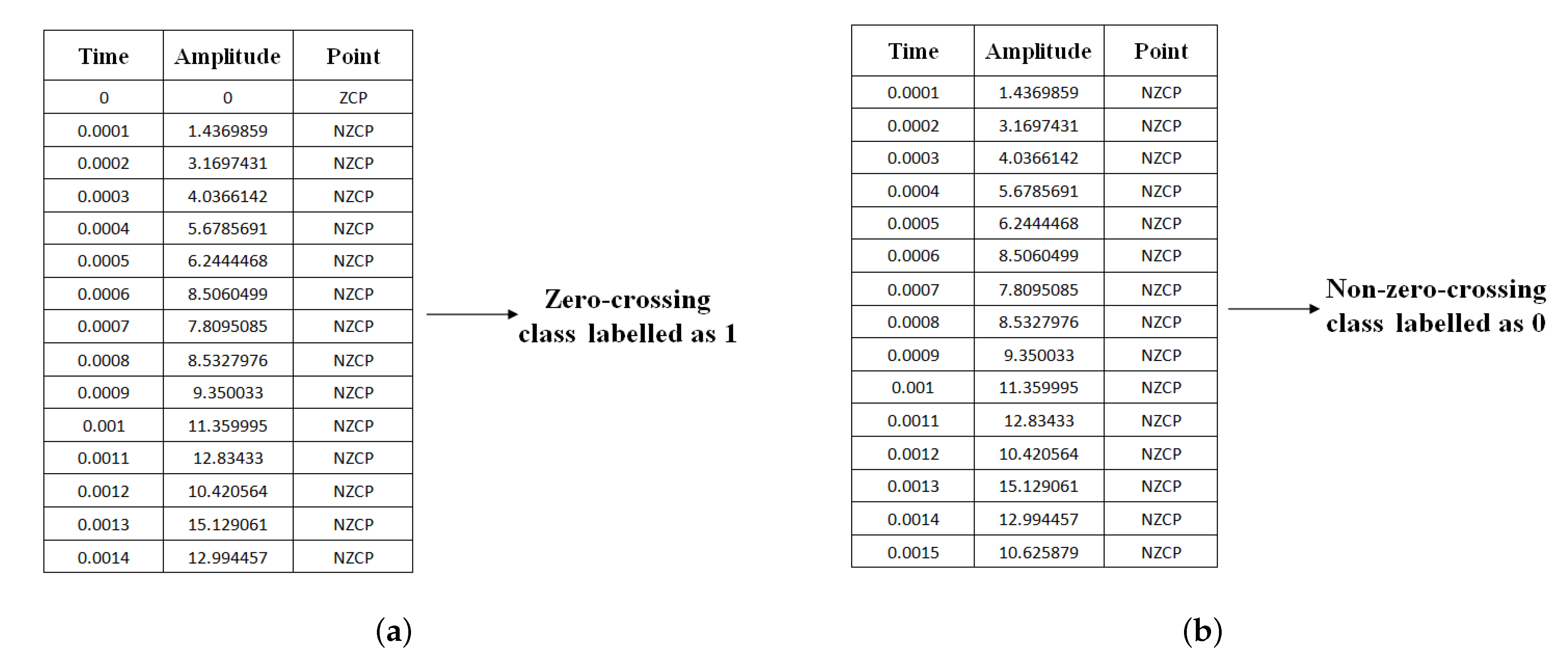
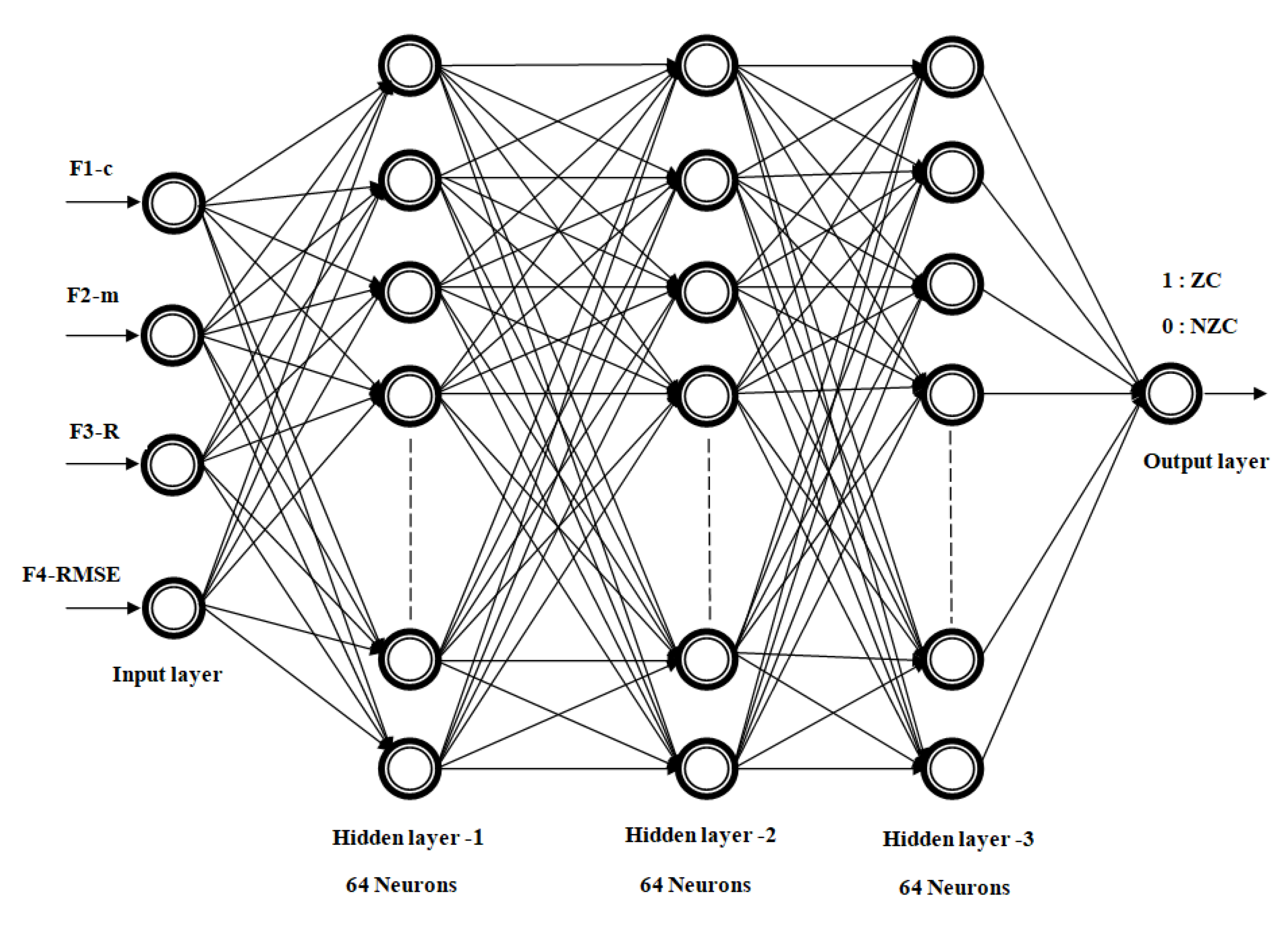
All the methodologies mentioned above provide valuable contributions to the ZCP problem. However, to improve the accuracy in predicting the true ZCPs, a new deep neural network (DNN) based machine learning model is developed in this paper. In order to make this DNN model more generalized, a variety of distorted signals are generated and extensive features such as slope, y-intercept, correlation and root mean square are extracted and used as dataset samples.
The main motivation for this work is to identify the most accurate zero-crossing points of distorted voltage signals for proper protection of a power system using switch-gear equipment and efficient power conversion by generating proper triggering pulses in conversion circuits.
The main contributions of this paper are as follows:
  • A properly tuned DNN model is developed for accurate ZCP detection.
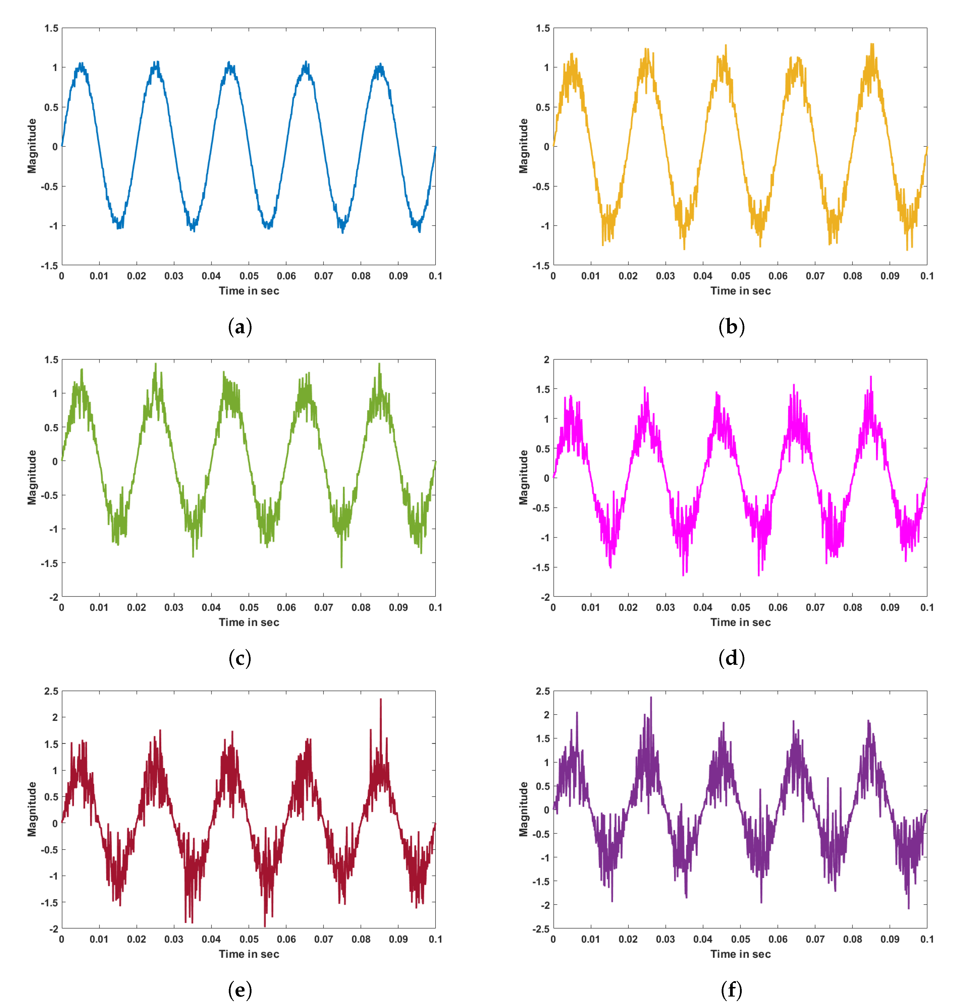
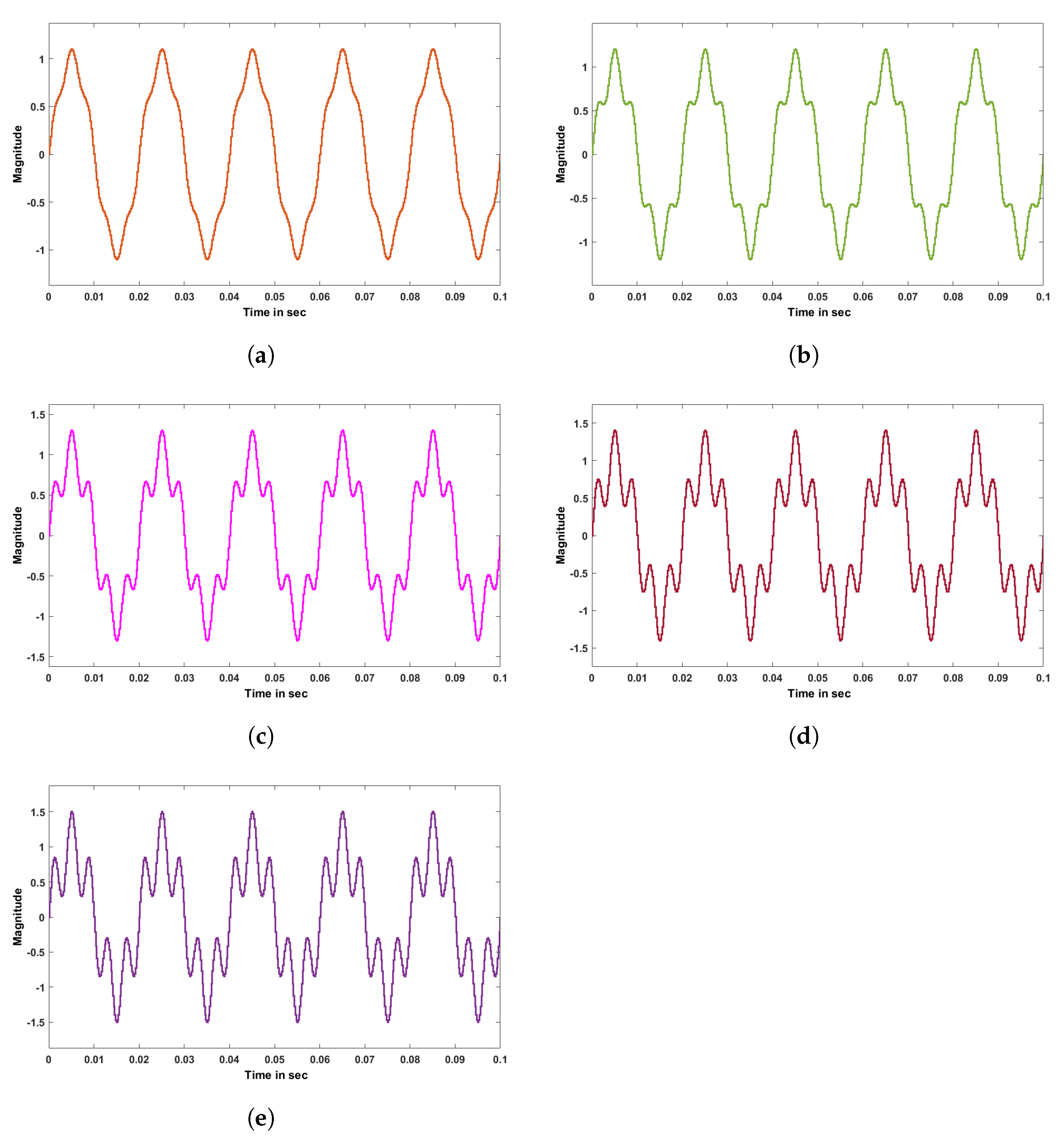
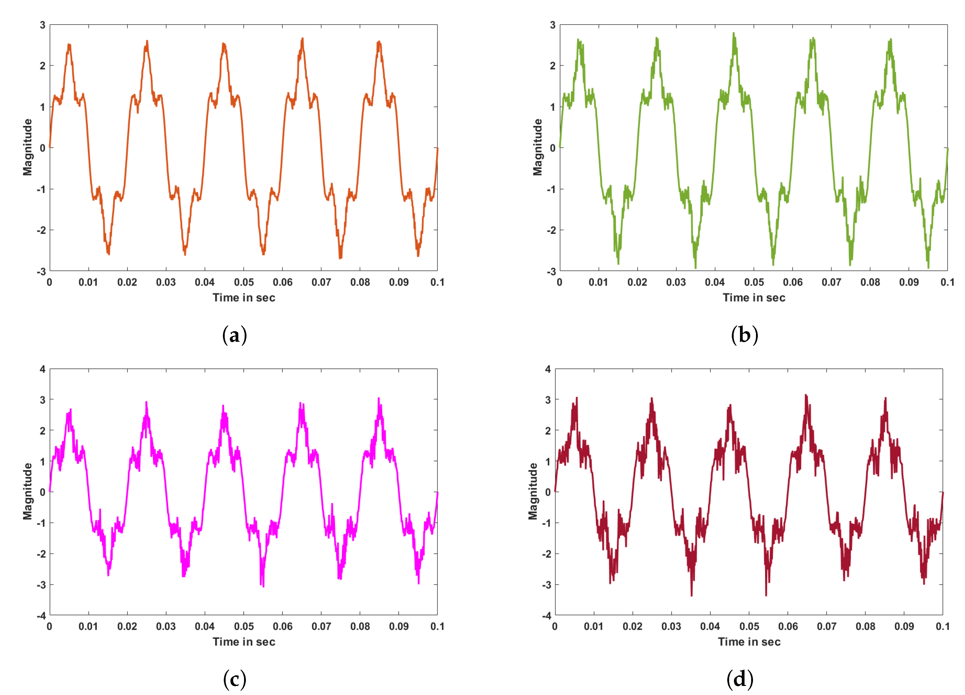
  • Four new datasets are created with a variety of distorted sinusoidal signals by considering noise levels from 5% to 15% and THD levels from 10% to 50%.
The remaining part of this paper is structured as follows: Section 2 presents a methodology that includes DNN model configuration and dataset preparation, Section 3 demonstrates results analysis and Section 4 describes conclusions.

2. Methodology

Four new datasets are created using MATLAB software for the ZCP detection problem and are available in [19]. The first dataset developed using distorted sinusoidal signals with noise levels from 10% to 50% consists of 4936 samples. The second dataset developed using distorted sinusoidal signals with THD levels from 10% to 50% consists of 4436 samples. The third dataset developed using distorted sinusoidal signals with noise levels from 10% to 40% and with THD level 50% consists of 3949 samples. The fourth dataset developed using distorted sinusoidal signals with noise levels from 5% to 20% consists of 3949 samples.

2.1. Dataset Formulation

Data samples are collected every 100 microseconds duration over 5 cycles. The complete dataset preparation mechanism is presented in Figure 1.

Sinusoidal Signals Used for Data Preparation

The data of the various sinusoidal voltage signals with noise (5 to 50%) is extracted by generating the signals in MATLAB as shown in Figure 2. In this paper, distorted sinusoidal signals are generated with white gaussian noise. Similarly, the data of the various sinusoidal voltage signals with total harmonic distortion from 10% to 50% is extracted by generating the signals in MATLAB as shown in Figure 3. Distorted sinusoidal signals are generated by adding unity amplitude fundamental signal with 5th order harmonic signals with varying amplitude from 0.1 to 0.5. THD of these distorted signals is estimated using FFT analysis based on equation
T H D = h = 2 V h 2 V f
where V h is RMS value of harmonic voltage signal and V f is RMS value of fundamental voltage signal.
In the same way, a few more sinusoidal signals were generated in MATLAB with a combination of both noise and harmonics as shown in Figure 4.

2.2. Windowing of Data Points in Distorted Sinusoidal Signal

Data samples extracted from various signals are formed into data windows of a specific length. The best window size (i.e., number of data points for each data window) should be preferred for better accuracy of the classification model. The number of data points in a particular window for calculating features represents the window size. Different window sizes of 5, 10, 12 and 15 data points are used to train the model. For a 50 Hz signal with distinct levels of harmonic distortion and noise, the greatest accuracy is obtained for the data window with 15 data points in the classification of zero-crossing and non-zero-crossing points. Therefore, the window with 15 data points is used for all the tests that are carried out further. Each data window is classified into two classes, as ZCP class or non-zero-crossing point (NZCP) class based on the availability of ZCP in that window. ZCP class is labelled as 1 and NZCP class is labelled as 0. Date sampling based on window size 15 along with its class is shown in Figure 5.

2.3. Feature Extraction

Complete distorted sinusoidal signal data points over 5 cycles are split into multiple sets based on the sliding window approach. Each set consists of 15 data points since the window size is considered as 15. Four features called slope (m), intercept (c), correlation coefficient (R) and root mean square error (RMSE) are extracted from each set that consists of 15 data samples by comparing unity amplitude fundamental signal using below equations
m = n i = 1 n v k t k i = 1 n t k i = 1 n v k n i = 1 n ( t k ) 2 ( i = 1 n ( t k ) 2 )
c = i = 1 n v k ( i = 1 n ( t k ) 2 ) ( i = 1 n t k ) ( i = 1 n t k v k ) n i = 1 n ( t k ) 2 ( i = 1 n ( t k ) 2 )
R = n i = 1 n v k u k i = 1 n u k i = 1 n v k ( n i = 1 n ( u k ) 2 ( i = 1 n ( u k ) 2 ) ) ( n i = 1 n ( v k ) 2 ( i = 1 n ( v k ) 2 ) )
R o o t M e a n S q u a r e E r r o r ( R M S E ) = i = 1 n ( u k v k ) 2 n
where m is slope, c is intercept, R is correlation coefficient, n is number of samples, t k is time value of k t h data point, v k is voltage magnitude of distorted signal at time t k and U k is voltage magnitude of unity fundamental signal at time t k .
These four features are the input features for the selected window. If ZCP exists within the window then the class label (output variable) is 1, i.e., ZCP class. If ZCP does not exist within the window then the class label is 0, i.e., NZCP class. Hence, every sample in the dataset consists of four input features and one output variable that represents the class.

2.4. Deep Neural Network

Deep neural networks (DNN) are the most accepted and essential machine learning model to solve either regression or classification problems [20]. Deep neural networks are an assembly of layers that can be mathematically described, in the literature, as a “network function” that associates an input tensor with an output tensor [21]. A DNN is developed to predict the zero-crossing point using four input features of a distorted sinusoidal signal, i.e., slope, intercept, correlation and RMSE. The complete architecture of DNN used in this paper for accurate prediction of ZCP class is shown in Figure 6 and the model parameters are presented in Table 1. In the proposed DNN model, the ReLU activation function is used in hidden layers, whereas the sigmoid activation function is used in the output layer. Mathematical modeling of ReLU [22] and sigmoid activation functions [23] are
f ( x ) = m a x ( 0 , x )
g ( x ) = 1 1 + e x
Adam optimizer [24,25] is used to train the DNN model by considering minimization of the binary cross-entropy loss function shown below.
L = 1 n i = 1 n ( y i l o g ( p i ) + ( 1 y i ) l o g ( 1 p i ) )
where y i is actual class and p i is predicted class.
Accuracy of the proposed DNN model on various datasets is evaluated using:
A c c u r a c y = T P + T N T P + T N + F P + F N
where TP is the number of samples correctly identified as ZCP, TN is the number of samples correctly identified as NZCP, FN is the number of samples incorrectly identified as NZCP and FP is the number of samples incorrectly identified as ZCP.

Training and Testing Strategy

All the data samples in each dataset are split into two groups to train and test the DNN model by considering the test data size of 5%. The data split is performed randomly, and no duplicate samples are present between training and testing data. DNN models are trained and tested with four datasets independently. Starting weights of the DNN model while training with each dataset are different and these are generated randomly at beginning of the algorithm. DNN models are trained and tested on each dataset 10 times with different starting weights but with the same training and testing data. The best accuracy model among all simulations is considered for the prediction of ZCP class. In this paper, the DNN models are trained with the same training data but different initial weights for 10 times. The DNN model with the best training and testing accuracy over 10 runs is presented in the results.

3. Results

The dataset that is created, as per the discussion in Section 3, is for the training and testing of DNN models. Statistical features of all ZCP datasets, which are Dataset-1: noise levels 10% to 50%, Dataset-2: THD levels 10% to 50%, Dataset-3: noise levels 10% to 40% with THD level 50% and Dataset-4: Noise levels 5% to 20%, have been used to train the DNN model presented in Table 2, Table 3, Table 4 and Table 5 respectively. The back-propagation through time (BPTT) algorithm with the Adam optimizer is used to train the proposed DNN model. The proposed DNN model is being implemented and tested in Google Colab.
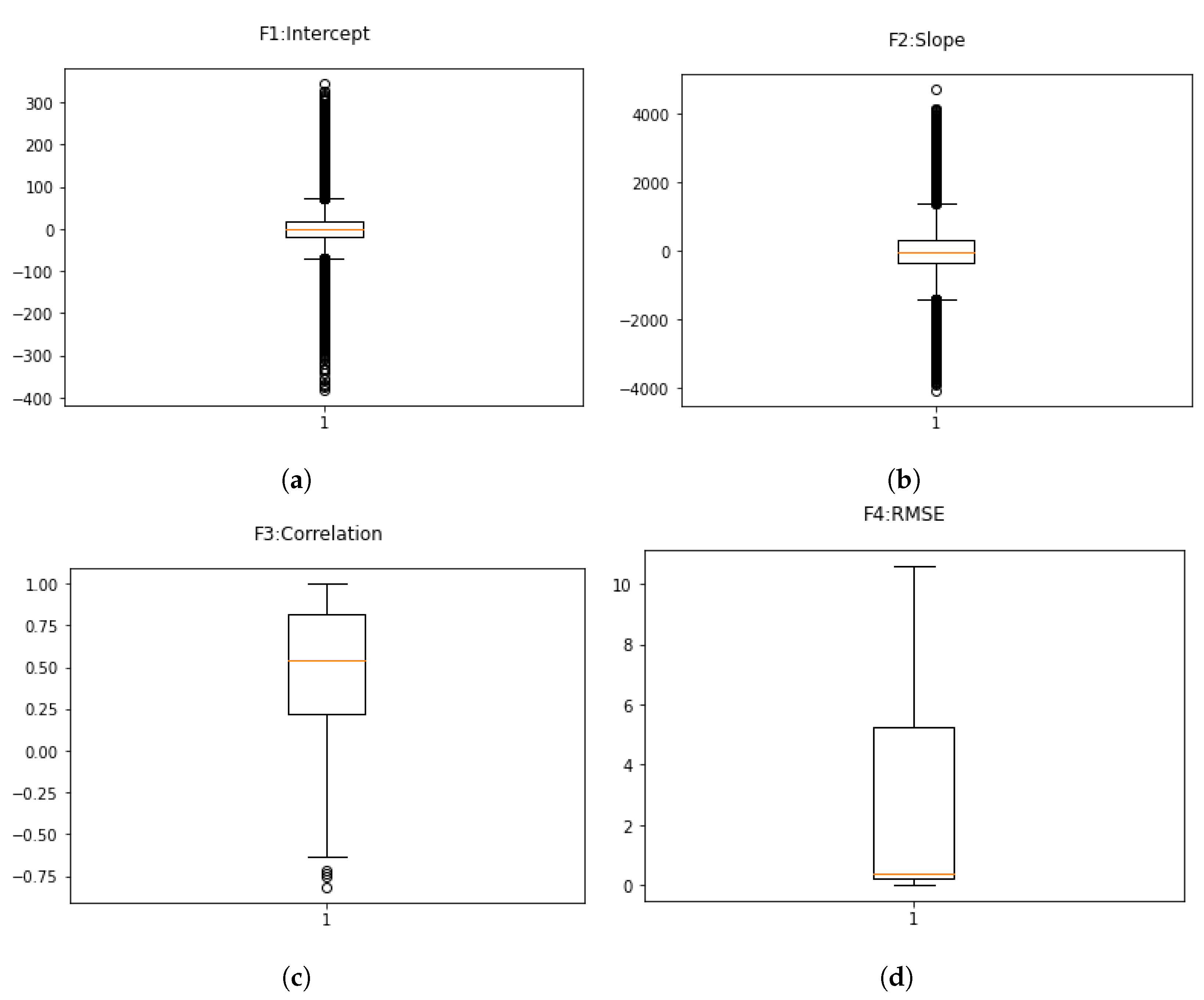
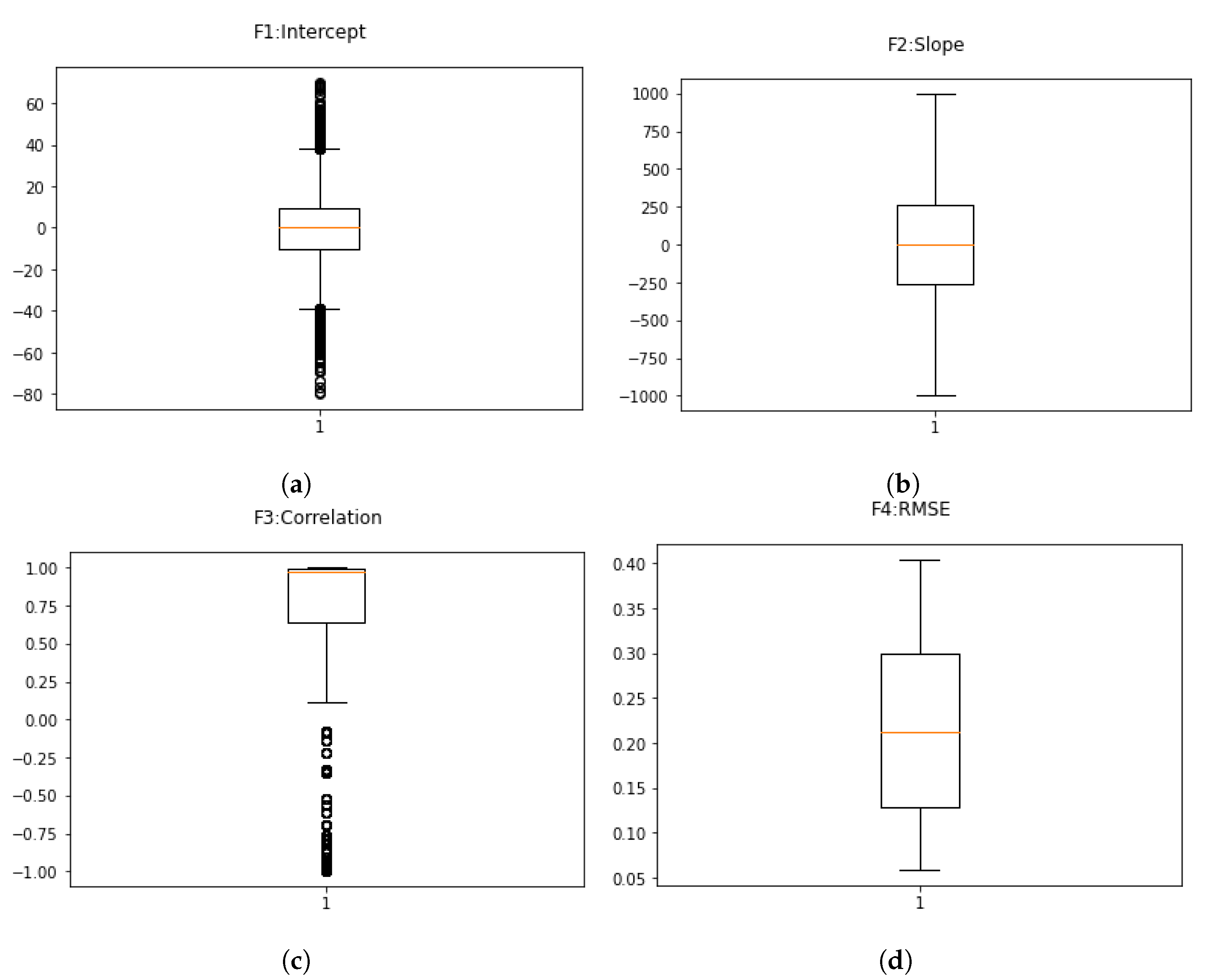
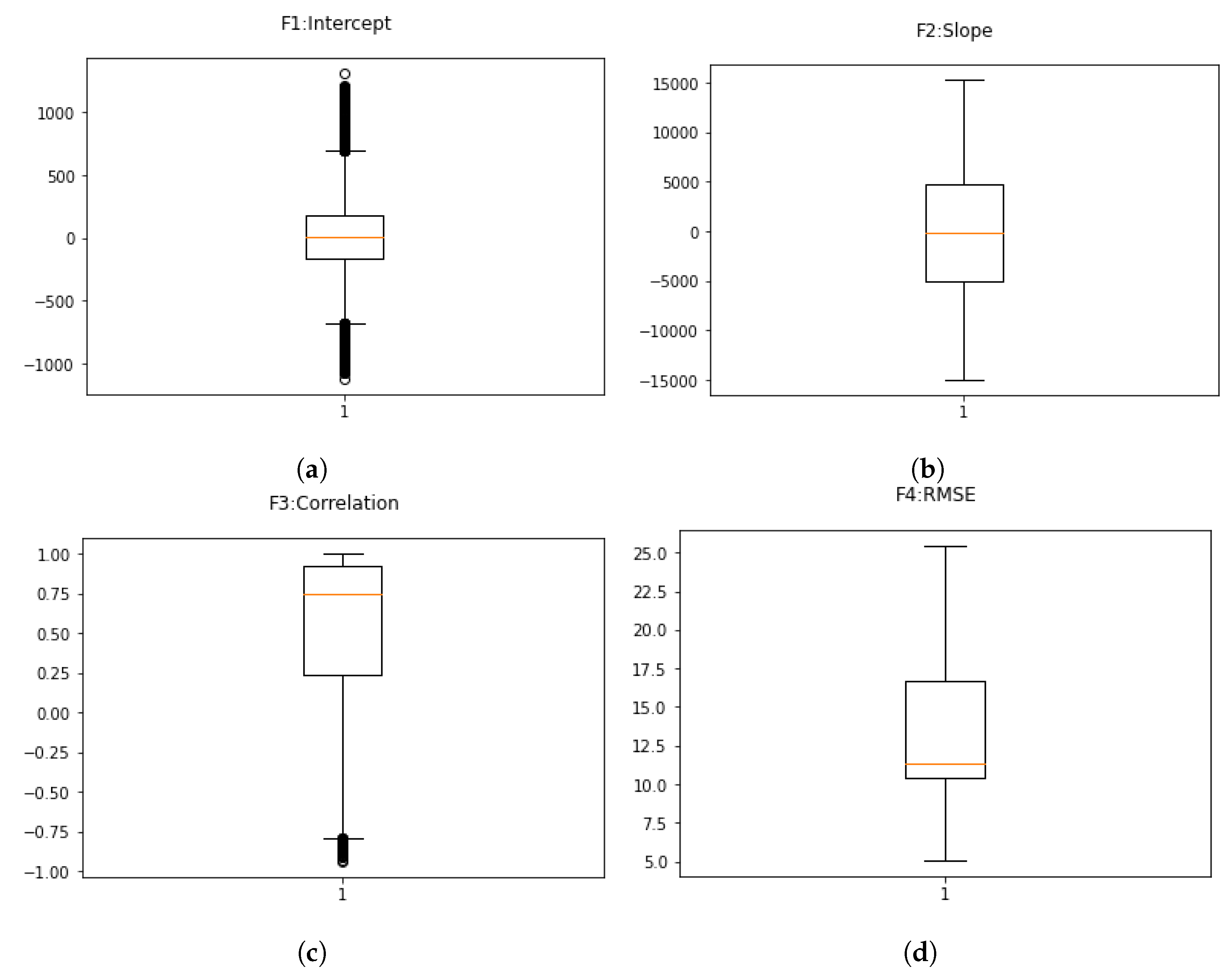
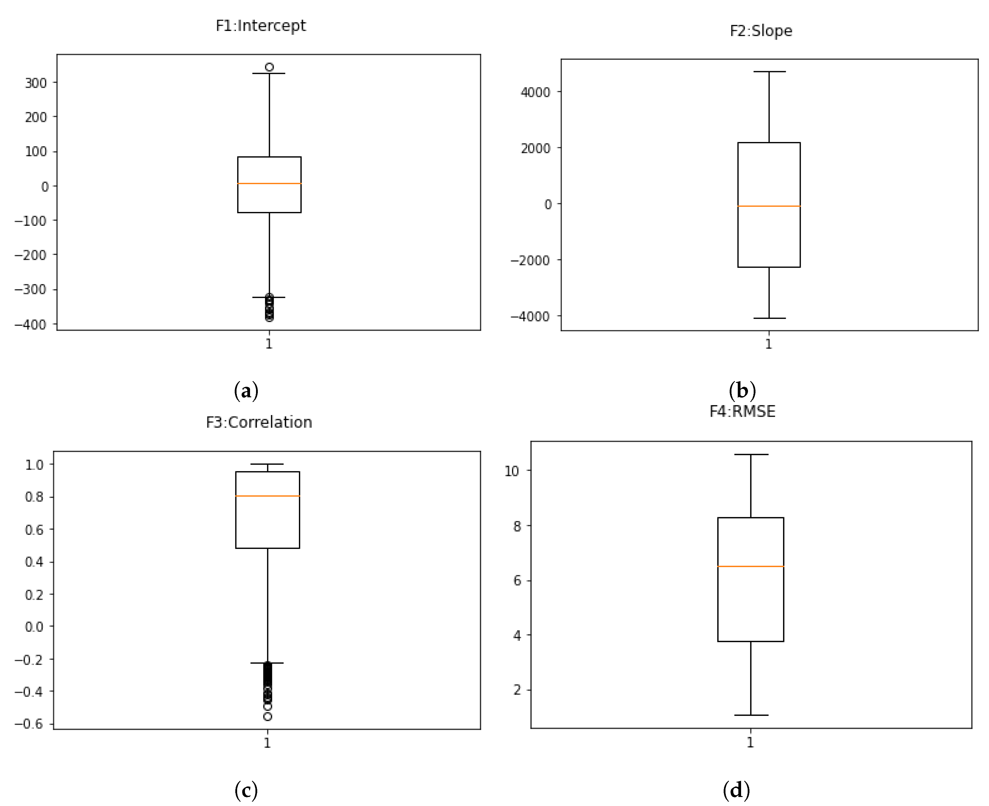
Box plots are used to identify the outliers against each input feature in every dataset mentioned above. Box plots against each feature for Dataset-1, Dataset-2, Dataset-3 and Dataset-4 are shown in Figure 7, Figure 8, Figure 9 and Figure 10, respectively. From all these plots, it has been observed that features in all datasets, such as intercept, correlation and slope, have outliers as data exist below the 25% interquartile range and above the 75% interquartile range. These outliers are due to spikes in distorted signals due to noise and harmonics and cannot be removed from data to make the model predict zero-crossing points under noise and harmonics.
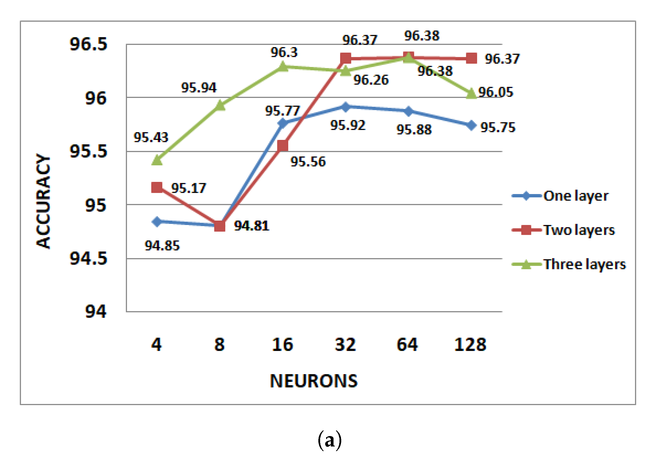
All four datasets that contain four input features and one output label are used to train the DNN model. The training accuracy of the DNN model against each variety of datasets for various hidden neurons and hidden layers combinations are shown in 
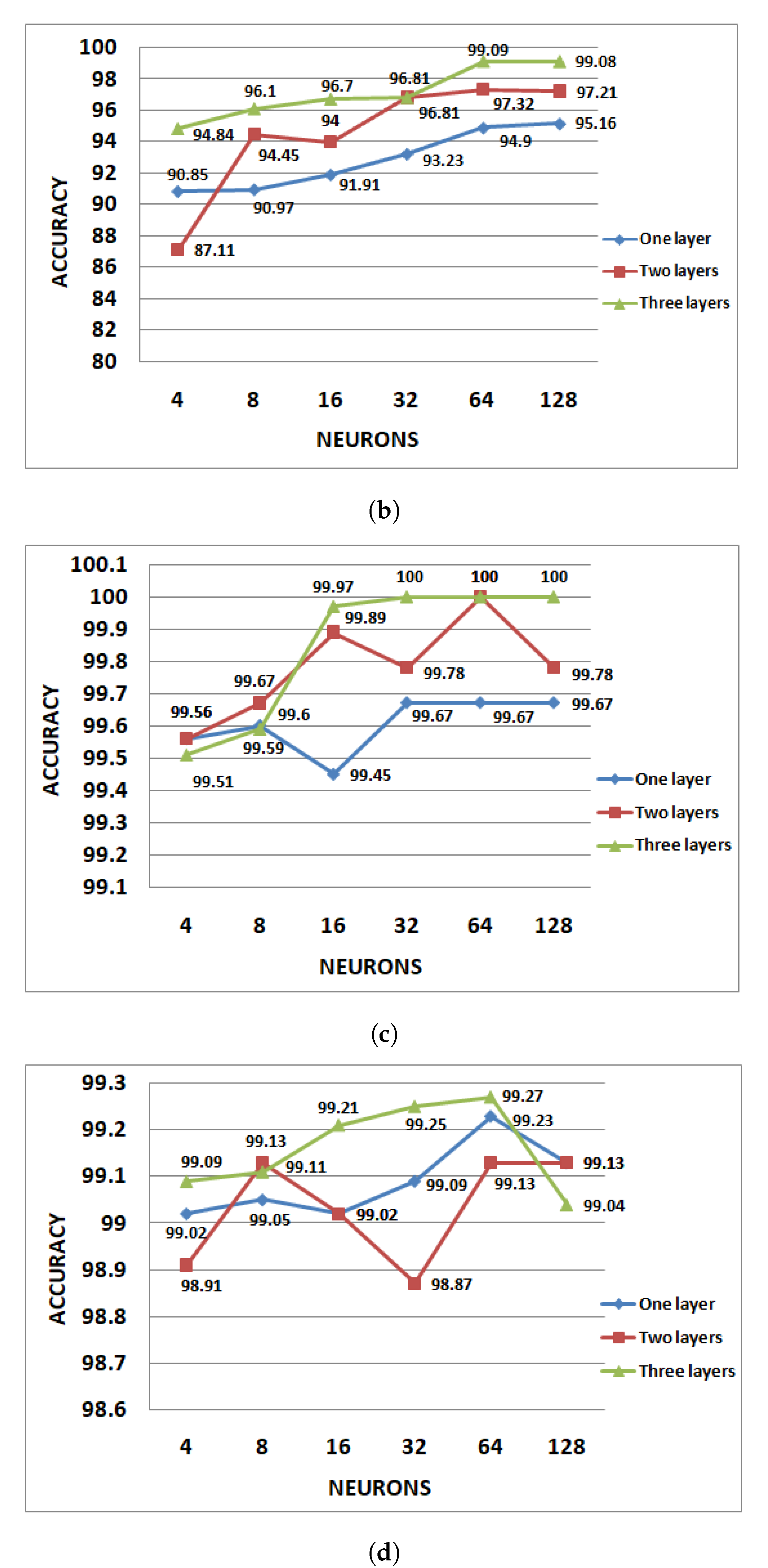
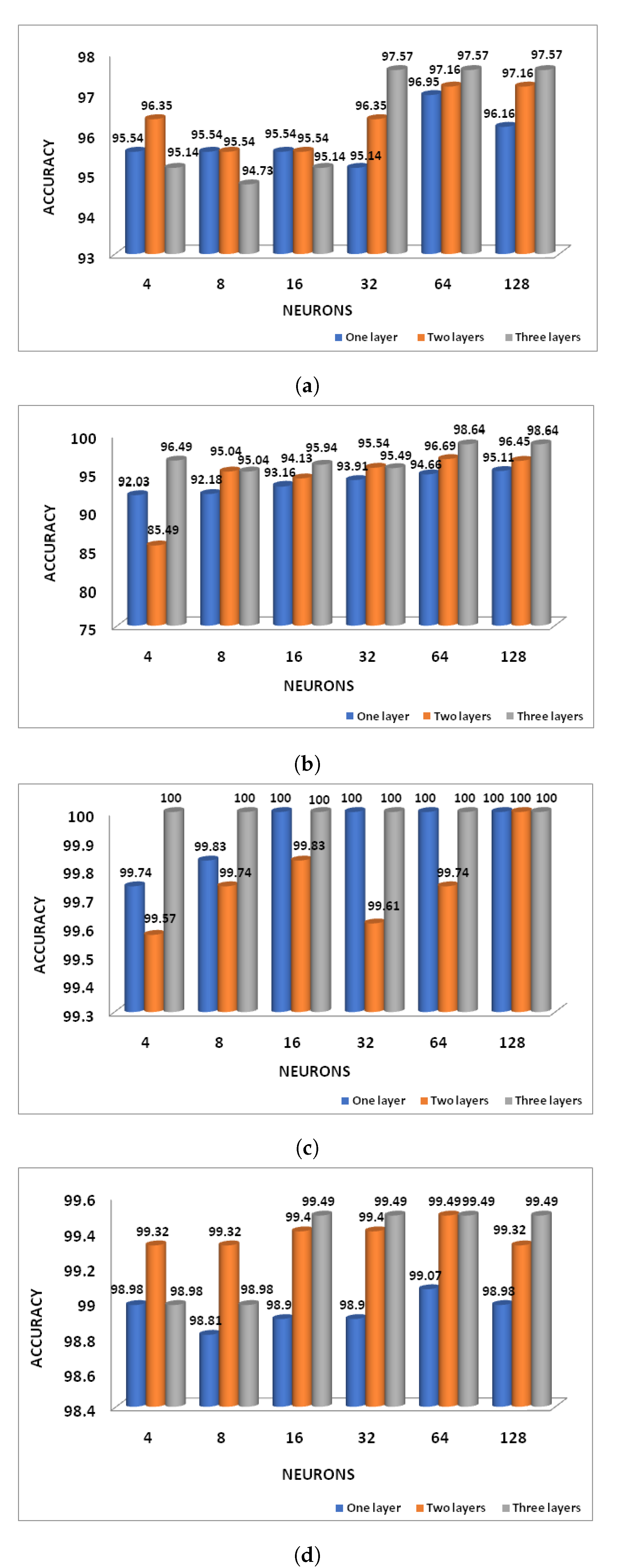
Figure 11. From the figure, it has been observed that the DNN model’s training performance is good with maximum accuracy with 3 hidden layers and 64 hidden neurons. Similarly, the testing accuracy of the DNN model against each variety of datasets for various hidden neurons and hidden layers combinations is shown in Figure 12. From the figure, it has been observed that the DNN model’s testing performance is good with maximum accuracy using 3 hidden layers and 64 hidden neurons.
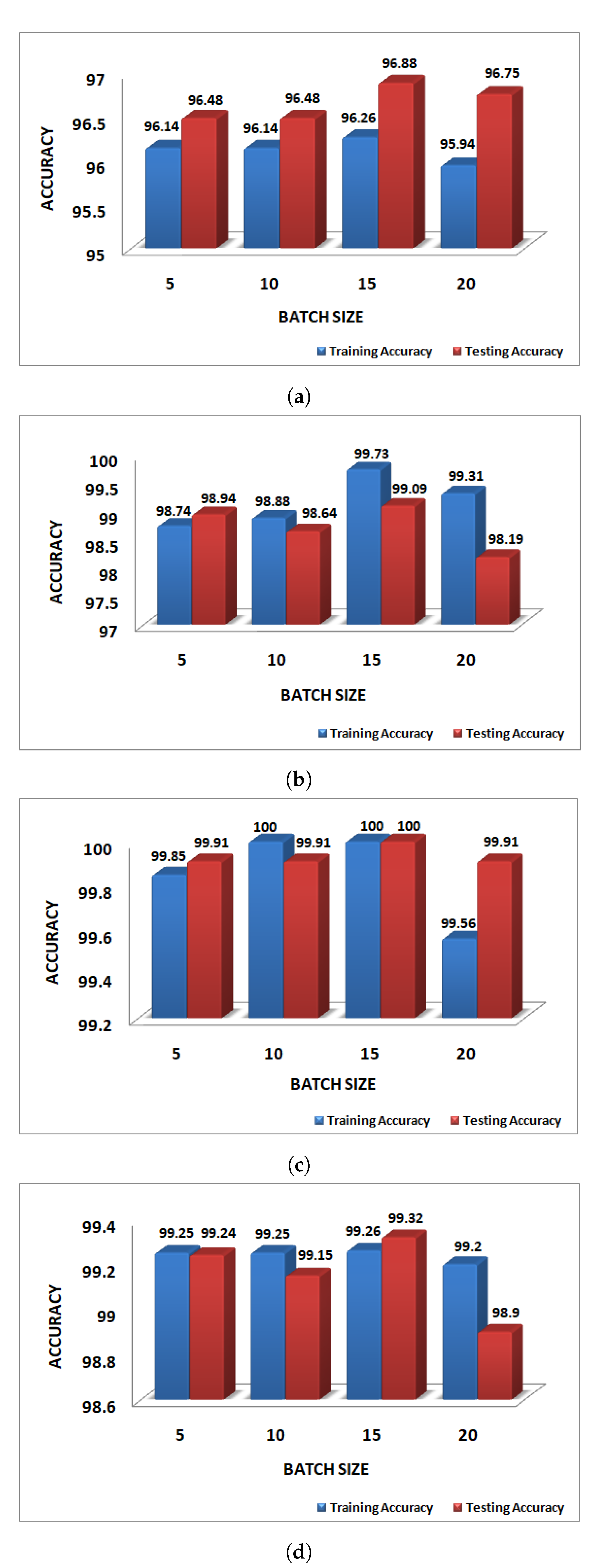
The proposed DNN model with 3 hidden layers and 64 hidden neurons is trained with various batch sizes on all the datasets mentioned in this paper, and accuracy levels for each batch size are presented in Figure 13. From Figure 13, it has been observed that the DNN model trained with a batch size of 15 provides good training accuracy of 96.26%, 99.73%, 100% and 99.26% and testing accuracy of 96.88%, 99.73%, 100% and 99.32% on Dataset-1, Dataset-2, Dataset-3 and Dataset-4, respectively.
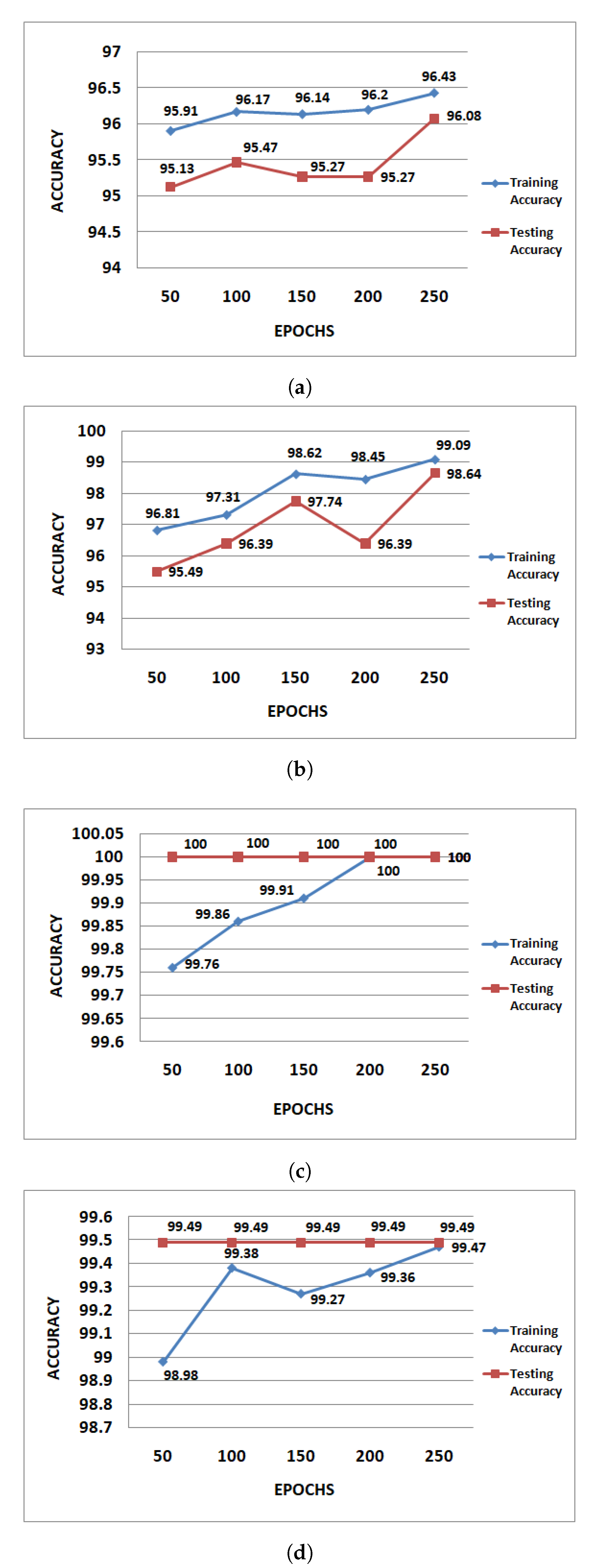
The proposed DNN model with 3 hidden layers and 64 hidden neurons is trained with various epoch sizes on all the datasets mentioned in this paper, and accuracy levels for each epoch size are presented in Figure 14. From Figure 14, it has been observed that the DNN model trained with an epoch size of 250 provides good training accuracy of 96.43%, 99.09%, 100% and 99.47% and testing accuracy of 96.08%, 98.64%, 100% and 99.49% on Dataset-1, Dataset-2, Dataset-3 and Dataset-4, respectively.
The proposed DNN model with 3 hidden layers, 64 hidden neurons and 250 epochs for all the datasets mentioned in this paper is trained with various window sizes as presented in Table 6. From Table 6, it can be observed that the proposed DNN model performs better for all the datasets with window size 15.
The proposed model with 3 hidden layers, 64 hidden neurons and 250 epochs for all the datasets mentioned in this paper with a window size of 15 data points is trained and tested 10 times. The accuracies for all the simulations are presented in Table 7. The best accuracy among all the 10 simulations was chosen as the final accuracy for respective datasets.

4. Discussion

The proposed DNN model with 3 hidden layers and 64 hidden neurons trained with a batch size of 15 and epoch size of 250 is used to predict the zero-crossing point class in real time as an optimal model. The proposed DNN model is validated by comparing it with some existing models, such as decision tree [26] and support vector machine (SVM) [27], as shown in Figure 15. From Figure 15, it has been observed that the training accuracy of the proposed model is a bit low if only either noisy or THD distorted signals are considered, but if the signal is highly distorted due to both noise and harmonics then the proposed model learning is good with better training accuracy. However, the proposed model is more generalized in comparison with decision tree and support vector machine, with better testing accuracy of 97.97%, 98.87%, 100% and 99.5% on Dataset-1, Dataset-2, Dataset-3 and Dataset-4, respectively, and that is required for real-time deployment.

5. Conclusions

Zero-crossing point detection is an essential task in various power system applications, such as grid synchronization, and power electronics applications, such as firing pulse generation for switching devices. The proposed good accuracy DNN model to predict the zero-crossing point can be used in the mentioned applications.
In this paper, four datasets with different noise levels and THD values are developed and used to train the DNN model for the accurate prediction of ZCP. A final DNN model with good accuracy was developed after tuning the hyper-parameters such as hidden layers, hidden neurons, batch size, window size and epochs.
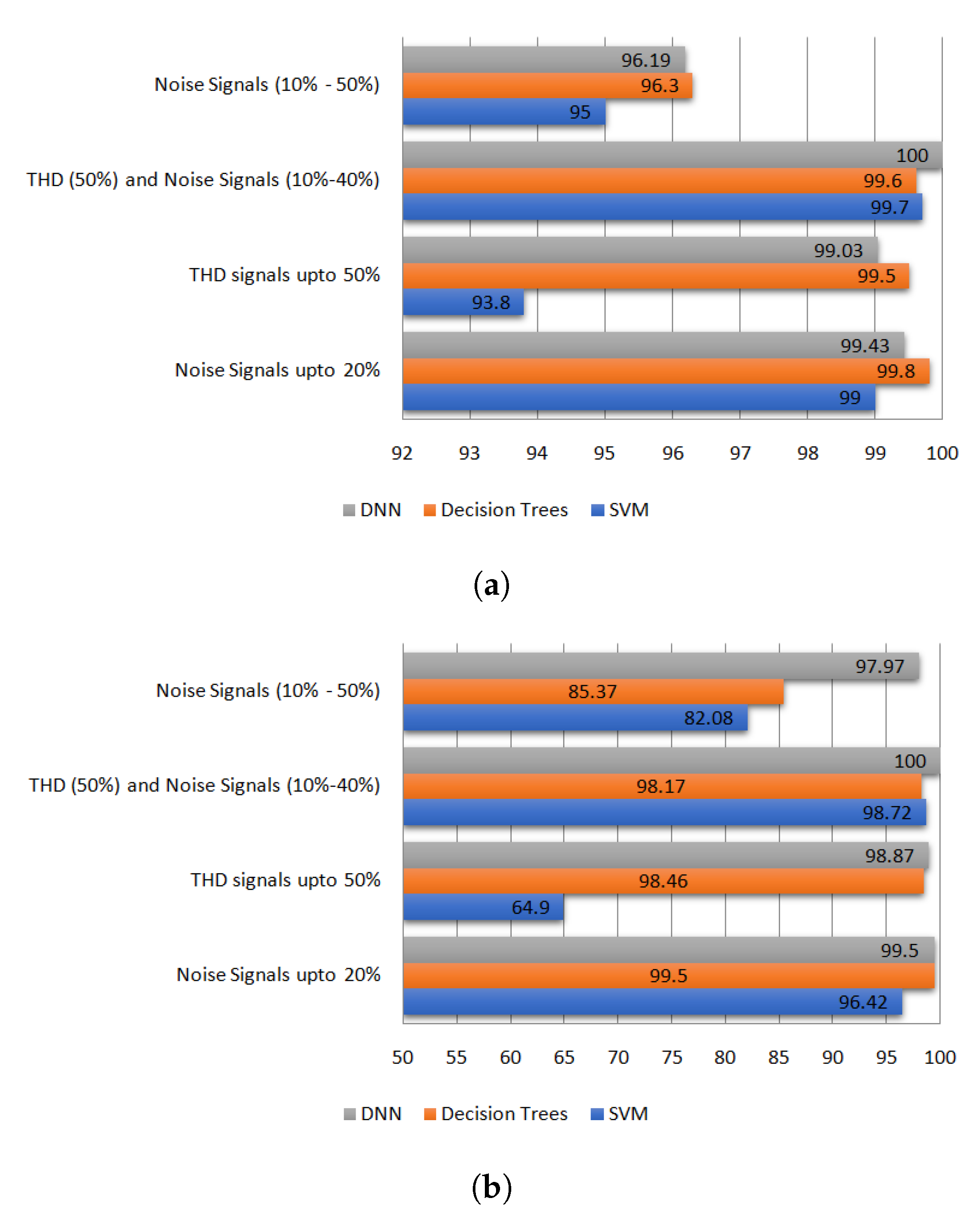
In this paper, a new DNN model with 3 hidden layers and 64 hidden neurons in each hidden layer is developed and ZCP classes were predicted with good accuracy in comparison with decision tree and SVM. The DNN model with a highly distorted signal, i.e., the signal that is distorted due to both noise and harmonics, has high accuracy in both training and testing as the model is well generalized with the high variance data. The proposed DNN model can predict the ZCP well on highly distorted signals. This work can be further extended by considering the distorted sinusoidal voltage with voltage sag and swells.

Author Contributions

V.V. and B.R.E. constructed the research theories and methods, developed the basic idea of the study, performed the computer simulation and analyses and conducted the preliminary research; S.R.S. worked on proofreading this article; V.V., S.R.S. and B.R.E. worked on document preparation; V.V. served as the head researcher in charge of the overall content of this study as well as modifications made. All authors have read and agreed to the published version of the manuscript.

Funding

Woosong University’s Academic Research Funding—2021.

Informed Consent Statement

Not applicable.

Data Availability Statement

The datasets generated during and/or analyzed during the current study are available in the Mendeley Data repository, https://data.mendeley.com/datasets/jbwy5fjcdj/2 (accessed on 7 November 2021).

Acknowledgments

We thank SR University, Warangal (Formerly, S R Engineering College Warangal), Telangana State, India, and Woosong University, South Korea, for supporting us during this work.

Conflicts of Interest

The authors declare that they have no conflict of interest.

References

  1. Jaalam, N.; Rahim, N.; Bakar, A.; Tan, C.; Haidar, A.M. A comprehensive review of synchronization methods for grid-connected converters of renewable energy source. Renew. Sustain. Energy Rev. 2016, 59, 1471–1481. [Google Scholar] [CrossRef] [Green Version]
  2. Huang, C.H.; Lee, C.H.; Shih, K.J.; Wang, Y.J. A robust technique for frequency estimation of distorted signals in power systems. IEEE Trans. Instrum. Meas. 2010, 59, 2026–2036. [Google Scholar] [CrossRef]
  3. Ghorbani, M.J.; Mokhtari, H. Impact of Harmonics on Power Quality and Losses in Power Distribution Systems. Int. J. Electr. Comput. Eng. 2015, 5, 2088–8708. [Google Scholar] [CrossRef]
  4. Veeramsetty, V.; Mohnot, A.; Singal, G.; Salkuti, S.R. Short Term Active Power Load Prediction on A 33/11 kV Substation Using Regression Models. Energies 2021, 14, 2981. [Google Scholar] [CrossRef]
  5. Veeramsetty, V.; Singal, G.; Badal, T. Coinnet: Platform independent application to recognize Indian currency notes using deep learning techniques. Multimed. Tools Appl. 2020, 79, 22569–22594. [Google Scholar] [CrossRef]
  6. Mendonça, T.R.; Pinto, M.F.; Duque, C.A. Least squares optimization of zero crossing technique for frequency estimation of power system grid distorted sinusoidal signals. In Proceedings of the 2014 11th IEEE/IAS International Conference on Industry Applications, Juiz de Fora, Brazil, 7–10 December 2014; pp. 1–6. [Google Scholar]
  7. Valiviita, S. Zero-crossing detection of distorted line voltages using 1-b measurements. IEEE Trans. Ind. Electron. 1999, 46, 917–922. [Google Scholar] [CrossRef]
  8. Gupta, A.; Thakur, R.; Murarka, S. An efficient approach to zero crossing detection based on opto-coupler. Int. J. Eng. Res. Appl. 2013, 3, 834–838. [Google Scholar]
  9. Wang, J.; Yoshimura, K.; Kurokawa, F. Zero-crossing point detection using differentiation circuit for boundary current mode PFC converter. In Proceedings of the 2015 IEEE 2nd International Future Energy Electronics Conference (IFEEC), Taipei, Taiwan, 1–4 November 2015; pp. 1–6. [Google Scholar]
  10. Ghosh, M.; Koley, C.; Roy, N.K. Robust support vector machine-based zero-crossing detector for different power system applications. IET Sci. Meas. Technol. 2019, 13, 83–89. [Google Scholar] [CrossRef]
  11. Wang, Z.; Wu, S.; Wang, M.; Yang, Y.; Luan, X.; Li, W. Zero-Crossing Detection Algorithm Based on Narrowband Filtering. In Proceedings of the 2020 IEEE 3rd Student Conference on Electrical Machines and Systems (SCEMS), Jinan, China, 4–6 December 2020; pp. 189–193. [Google Scholar]
  12. Patil, T.; Ghorai, S. Robust zero-crossing detection of distorted line voltage using line fitting. In Proceedings of the 2016 International Conference on Electrical, Electronics, Communication, Computer and Optimization Techniques (ICEECCOT), Mysuru, India, 9–10 December 2016; pp. 92–96. [Google Scholar]
  13. Zhu, W.J.; Xu, K.J.; Fang, M.; Shen, Z.W.; Tian, L. Variable ratio threshold and zero-crossing detection based signal processing method for ultrasonic gas flow meter. Measurement 2017, 103, 343–352. [Google Scholar] [CrossRef]
  14. Yang, L.; Zhu, Z.; Bin, H.; Zhang, Z.; Gong, L. Safety Operation Area of Zero-Crossing Detection-Based Sensorless High-Speed BLDC Motor Drives. IEEE Trans. Ind. Appl. 2020, 56, 6456–6466. [Google Scholar] [CrossRef]
  15. Fang, Z.; Su, R.; Hu, L.; Fu, X. A simple and easy-implemented time-of-flight determination method for liquid ultrasonic flow meters based on ultrasonic signal onset detection and multiple-zero-crossing technique. Measurement 2021, 168, 108398. [Google Scholar] [CrossRef]
  16. Yu, J.; Liu, M.; Song, D.; Yang, J.; Su, M. A soft-switching control for cascaded buck-boost converters without zero-crossing detection. IEEE Access 2019, 7, 32522–32536. [Google Scholar] [CrossRef]
  17. Jumrianto, J.; Royan, R. Proteus ISIS simulation for power factor calculation using zero crossing detector. J. Mechatron. Electr. Power Veh. Technol. 2021, 12, 28–37. [Google Scholar] [CrossRef]
  18. Rahman, D.; Awal, M.; Islam, M.S.; Yu, W.; Husain, I. Low-latency High-speed Saturable Transformer based Zero-Crossing Detector for High-Current High-Frequency Applications. In Proceedings of the 2020 IEEE Energy Conversion Congress and Exposition (ECCE), Detroit, MI, USA, 11–15 October 2020; pp. 3266–3272. [Google Scholar]
  19. Zero-crossing Point Detection Dataset-Distorted Sinusoidal Signals. Available online: https://data.mendeley.com/drafts/jbwy5fjcdj (accessed on 5 October 2021).
  20. Veeramsetty, V.; Deshmukh, R. Electric power load forecasting on a 33/11 kV substation using artificial neural networks. SN Appl. Sci. 2020, 2, 1–10. [Google Scholar] [CrossRef] [Green Version]
  21. Lassance, C.; Gripon, V.; Ortega, A. Representing deep neural networks latent space geometries with graphs. Algorithms 2021, 14, 39. [Google Scholar] [CrossRef]
  22. Kulathunga, N.; Ranasinghe, N.R.; Vrinceanu, D.; Kinsman, Z.; Huang, L.; Wang, Y. Effects of Nonlinearity and Network Architecture on the Performance of Supervised Neural Networks. Algorithms 2021, 14, 51. [Google Scholar] [CrossRef]
  23. Pratiwi, H.; Windarto, A.P.; Susliansyah, S.; Aria, R.R.; Susilowati, S.; Rahayu, L.K.; Fitriani, Y.; Merdekawati, A.; Rahadjeng, I.R. Sigmoid Activation Function in Selecting the Best Model of Artificial Neural Networks. J. Phys. Conf. Ser. 2020, 1471, 012010. [Google Scholar] [CrossRef]
  24. Kingma, D.P.; Ba, J. Adam: A method for stochastic optimization. arXiv 2014, arXiv:1412.6980. [Google Scholar]
  25. Veeramsetty, V.; Chandra, D.R.; Salkuti, S.R. Short-term electric power load forecasting using factor analysis and long short-term memory for smart cities. Int. J. Circuit Theory Appl. 2021, 49, 1678–1703. [Google Scholar] [CrossRef]
  26. Myles, A.J.; Feudale, R.N.; Liu, Y.; Woody, N.A.; Brown, S.D. An introduction to decision tree modeling. J. Chemom. J. Chemom. Soc. 2004, 18, 275–285. [Google Scholar] [CrossRef]
  27. Suthaharan, S. Support vector machine. In Machine Learning Models and Algorithms for Big Data Classification; Springer: Berlin/Heidelberg, Germany, 2016; pp. 207–235. [Google Scholar]
Figure 1. Mechanism of data preparation.
Algorithms 14 00329 g001
Figure 2. Noise signals used for dataset preparation. (a) Noise level 5%. (b) Noise level 15%. (c) Noise level 20%. (d) Noise level 30%. (e) Noise level 40%. (f) Noise level 50%.
Algorithms 14 00329 g002
Figure 3. Sinusoidal signals with various THD levels used for dataset preparation. (a) THD level 10%. (b) THD level 20%. (c) THD level 30%. (d) THD level 40%. (e) THD level 50%.
Algorithms 14 00329 g003
Figure 4. Sinusoidal signals with various combinations of THD and noise levels used for dataset preparation. (a) Sinusoidal signal with THD level 50% and noise level 10%. (b) Sinusoidal signal with THD level 50% and noise level 20%. (c) Sinusoidal signal with THD level 50% and noise level 30%. (d) Sinusoidal signal with THD level 50% and noise level 40%.
Algorithms 14 00329 g004
Figure 5. Data sampling from sinusoidal signals with window size of 15. (a) Data window corresponds to ZCP class. (b) Data window corresponds to NZCP class.
Algorithms 14 00329 g005
Figure 6. DNN model topology.
Algorithms 14 00329 g006
Figure 7. Box plot for each input feature in Dataset-1 (noise level from 10% to 50%). (a) m. (b) c. (c) R. (d) RMSE.
Algorithms 14 00329 g007
Figure 8. Box plot for each input feature in Dataset-2 (THD level from 10% to 50%) (a) m. (b) c. (c) R. (d) RMSE.
Algorithms 14 00329 g008
Figure 9. Box plot for each input feature in Dataset-3 (noise level from 10% to 40% and THD level 50%). (a) m. (b) c. (c) R. (d) RMSE.
Algorithms 14 00329 g009
Figure 10. Box plot for each input feature in Dataset-4 (noise level from 5% to 20%). (a) m. (b) c. (c) R. (d) RMSE.
Algorithms 14 00329 g010
Figure 11. Training performance of DNN model on variety of data. (a) Noise level: 10 to 50 (Dataset-1). (b) THD level: 10 to 50 (Dataset-2). (c) THD level: 50, noise level: 10 to 40 (Dataset-3). (d) Noise level: 5 to 20 (Dataset-4).
Algorithms 14 00329 g011aAlgorithms 14 00329 g011b
Figure 12. Testing performance of DNN model on variety of data. (a) Noise level: 10 to 50 (Dataset-1). (b) THD level: 10 to 50 (Dataset-2). (c) THD level: 50, noise level: 10 to 40 (Dataset-3). (d) Noise level: 5 to 20 (Dataset-4).
Algorithms 14 00329 g012
Figure 13. Training and testing performance of DNN model with respect to various batch sizes. (a) Noise level: 10 to 50 (Dataset-1). (b) THD level: 10 to 50 (Dataset-2). (c) THD level: 50, noise level: 10 to 40 (Dataset-3). (d) Noise level: 5 to 20 (Dataset-4).
Algorithms 14 00329 g013
Figure 14. Training and testing performance of DNN model with respect to various number of epochs. (a) Noise level: 10 to 50 (Dataset-1). (b) THD level: 10 to 50 (Dataset-2). (c) THD level: 50, noise level: 10 to 40 (Dataset-3). (d) Noise level: 5 to 20 (Dataset-4).
Algorithms 14 00329 g014
Figure 15. Validation of proposed DNN model. (a) Validation of proposed model in terms of training accuracy. (b) Validation of proposed model in terms of testing accuracy.
Algorithms 14 00329 g015
Table 1. DNN model parameters.
LayerWeightsBiasParameters
125664320
24096644160
34096644160
464165
Total Trainable Parameters8705
Table 2. Statistical information of ZCP dataset with noise level from 10% to 50%.
ParametersF1: InterceptF2: SlopeF3: CorrelationF4: RMSE
count4935493549354935
mean0.906008423−18.6767290.4949008722.54591076
std84.859177911464.644720.3676751323.23948602
min−381.4180671−4065.341−0.8165512070.02172266
25%−16.76426941−350.02150.2171819320.21942497
50%0.891192436−11.9224650.541218870.40202541
75%18.56990887341.7554780.8208135325.27377613
max343.77621444706.997570.99929357210.5857103
Table 3. Statistical information of ZCP dataset with THD level from 10% to 50%.
ParametersF1: InterceptF2: SlopeF3: CorrelationF4: RMSE
count4435443544354435
mean−0.2809902161.57238 × 10−50.5954907070.211104753
std19.72465139383.26630920.6864122310.102681968
min−79.60710789−995.088821−0.9954887950.059104012
25%−9.873091003−261.78263840.6387779120.128286631
50%0.3362206640.0001104540.9743432240.212132057
75%9.320462957261.78243320.994127520.29862303
max69.65621941995.0888210.9998312740.403321083
Table 4. Statistical information of ZCP dataset with THD level 50% and noise level from 10% to 40%.
ParametersF1: InterceptF2: SlopeF3: CorrelationF4: RMSE
count3948394839483948
mean7.9240602−155.896040.51539508413.2242
std375.93209826605.029610.5231169444.916469
min−1123.05498−14989.989−0.9391476655.080782
25%−167.2859958−5086.1920.23811069810.42127
50%9.096503124−186.746140.742358511.35477
75%176.45626484785.2360.92423825616.65624
max1308.76821815297.00990.99972770125.40568
Table 5. Statistical information of ZCP dataset with noise level from 5% to 20%.
ParametersF1: InterceptF2: SlopeF3: CorrelationF4: RMSE
count3948394839483948
mean2.020936461−41.23897290.6797655955.954001746
std131.19027322264.2595330.3307594252.549789009
min−381.4180671−4065.34103−0.5537744341.078380672
25%−77.96528871−2258.869020.4828987583.754887732
50%5.359213813−74.61327310.8025487576.510990681
75%85.072772222183.0701730.9583382688.2692806
max343.77621444706.9975670.99974280510.58571031
Table 6. Accuracy of DNN model with respect to batch size.
SizeDataset-1Dataset-2Dataset-3Dataset-4
TrainingTestingTrainingTestingTrainingTestingTrainingTesting
595.3796.698.998.5610010098.599.5
1095.9697.5898.8398.3810010090.6392.46
1596.1997.9799.0398.8710010099.4399.5
2081.2385.7794.5195.9399.9110081.5579.69
Table 7. Training and testing accuracy on various simulation runs.
Dataset-1Dataset-2Dataset-3Dataset-4
RunTrainingTestingTrainingTestingTrainingTestingTrainingTesting
196.1595.5498.6498.1910010099.4199.49
296.1697.5798.7498.1910010099.4699.49
395.9697.1698.7897.2910010099.4699.49
496.1397.5499.0398.8710010099.4399.49
596.0397.5499.0298.6410010099.2299.5
695.9895.5498.9998.5410010099.4399.5
796.1996.7699.0398.5410010099.2599.5
896.1697.9798.9596.8410010099.4199.5
996.1497.9598.597.2910010099.4199.5
1096.1397.5799.0198.8610010099.4399.5
Best96.1997.9799.0398.8710010099.4399.5
Publisher’s Note: MDPI stays neutral with regard to jurisdictional claims in published maps and institutional affiliations.

