Article

Compensating Data Shortages in Manufacturing with Monotonicity Knowledge

1
Fraunhofer Institute for Industrial Mathematics ITWM, Fraunhofer-Platz 1, 67663 Kaiserslautern, Germany
2
Fraunhofer Institute for Machine Tools and Forming Technology IWU, Reichenhainer Straße 88, 09126 Chemnitz, Germany
3
Fraunhofer Institute for Mechanics of Materials IWM, Wöhlerstraße 11, 79108 Freiburg, Germany
*
Author to whom correspondence should be addressed.
Submission received: 19 October 2021 / Revised: 17 November 2021 / Accepted: 25 November 2021 / Published: 27 November 2021
(This article belongs to the Special Issue Optimization Algorithms and Applications at OLA 2021)

Abstract

:
Systematic decision making in engineering requires appropriate models. In this article, we introduce a regression method for enhancing the predictive power of a model by exploiting expert knowledge in the form of shape constraints, or more specifically, monotonicity constraints. Incorporating such information is particularly useful when the available datasets are small or do not cover the entire input space, as is often the case in manufacturing applications. We set up the regression subject to the considered monotonicity constraints as a semi-infinite optimization problem, and propose an adaptive solution algorithm. The method is applicable in multiple dimensions and can be extended to more general shape constraints. It was tested and validated on two real-world manufacturing processes, namely, laser glass bending and press hardening of sheet metal. It was found that the resulting models both complied well with the expert’s monotonicity knowledge and predicted the training data accurately. The suggested approach led to lower root-mean-squared errors than comparative methods from the literature for the sparse datasets considered in this work.

1. Introduction

Systematic decision making in manufacturing—such as finding optimal parameter settings for a manufacturing process—requires appropriate models for that process. In particular, such models have to be sufficiently accurate, and at the same time, sufficiently quick at evaluating. In principle, for many industrial processes, precise simulation models based on detailed physical modeling can be built. Yet, these so-called white-box models are typically too slow to be of any practical use in exploring the process parameter space and in eventually finding optimal process parameters (online and offline). In this respect, machine learning models can be very useful surrogates with short runtimes.
Conventional machine learning models are purely data-based (so-called black-box models). Accordingly, the predictive power of such models is generally bad if the underlying training data D = { ( x l , t l ) : l { 1 , , N } } are insufficient. Unfortunately, such data insufficiencies occur quite often, and they can come in one of the following forms: On the one hand, the available datasets can be too small and have too little variance in the input data points x 1 , , x N . This problem frequently occurs in manufacturing [1] because varying the process parameters beyond well-tested operating windows is usually costly. On the other hand, the output data t 1 , , t N can be too noisy.
Aside from potentially insufficient data, however, one often also has additional knowledge about the relation between the input variables and the responses to be learned. Such extra knowledge about the considered process is referred to as expert knowledge in the following. In [2], the interactions of users with software was tracked to capture their expert knowledge in a general form as training data for a classification problem. In [3], expert knowledge was used in the form of a specific algebraic relation between input and output to solve a parameter estimation problem with artificial neural networks. Such informed machine learning [4] techniques beneficially combine expert knowledge and data to build hybrid or gray-box models [5,6,7,8,9,10,11,12], which predict the responses more accurately than purely data-based models. In other words, by using informed machine learning techniques, one can compensate data insufficiencies with expert knowledge.
An important and common type of expert knowledge is prior information about the monotonicity behavior of the unknown functional relationship x y ( x ) to be learned. A large variety of concrete application examples with monotonicity knowledge can be found in ([13], Section 4.1) and ([14], Section 1), for instance. The present article exclusively deals with regression under such monotonicity requirements. For classification under monotonicity constraints, see, e.g., [14,15]. Along with convexity constraints, monotonicity constraints are probably the most intensively studied shape constraints [16] in the literature, and correspondingly, there exist plenty of different approaches to incorporate monotonicity knowledge in a machine learning model. See [17] for an extensive overview. Very roughly, these approaches can be categorized according to when the monotonicity knowledge is taken into account: in or only after the training phase. In the terminology of [4], this corresponds to the distinction between knowledge integration in the learning algorithm or in the final hypothesis.
A lot of methods—especially from the mathematical statistics literature, such as [18,19,20,21,22,23,24]—incorporate monotonicity knowledge only after training. These articles start with a purely data-based initial model, which in general does not satisfy the monotonicity requirements, and then monotonize this initial model according to a suitable monotonization procedure, such as projection [18,19,20,24], rearrangement [22,23,25] or tilting [21]. Among other things, it is shown in the mentioned articles that, in spite of noise in the output data, the arising monotonized models are close to the true relationship for sufficiently large training datasets. Summarizing, these articles show that for large datasets, noise in the output data can be compensated by monotonization to a certain extent.
In contrast to that, in some works, such as [13,17,26,27,28,29], monotonicity knowledge was incorporated already in training. In these articles, the monotonicity requirements were added as constraints—either hard [17,26,28,29] or soft [13,26]—to the data-based optimization of the model parameters. In [13,28], probabilistic monotonicity notions are used. In [26,27,28,29], support vector regressors in the linear-programming or the more standard quadratic-programming form, Gaussian process regressors or neural network models were considered, and the monotonicity of these models was enforced by constraints on the model derivatives at predefined sampling points [26,28,29] or on the model increments between predefined pairs of sampling points [27].
A disadvantage of the projection- and rearrangement-based approaches [22,23,24] from the point of view of manufacturing applications is that these methods are tailored to large datasets. Another disadvantage of these approaches is that the resulting models typically exhibit distinctive kinks, which are almost always unphysical. Additionally, the models resulting from the multidimensional rearrangement method by [23] are not guaranteed to be monotonic when trained on small datasets. A drawback of the tilting approach from [21] is that it is formulated and validated only for one-dimensional input spaces (intervals in R ). Accordingly, naively extending the non-adaptive discretization scheme from [21] to higher dimensions would result in long computation times. A downside of the in-training methods from [26,28,29] is that the sampling points at which the monotonicity constraints are imposed have to be chosen in advance (even though they need not coincide with the training data points).
With the method proposed in the present article, we address the aforementioned issues and shortcomings. In Section 2, our methodology for monotonic regression using semi-infinite optimization is introduced. It incorporates the monotonicity knowledge during training. Specifically, polynomial regression models are assumed for the input–output relationships to be learned. Since there is no after-training monotonization step in the method, our models are smooth, and in particular, do not exhibit kinks. Also, due to the employed adaptive discretization scheme, the method is computationally efficient also in higher dimensions. To our knowledge, such an adaptive scheme has not been applied to solve monotonic regression problems before, especially not in situations with sparse data. In Section 4, the method is validated by means of two applications to real-world processes which are both introduced in Section 3, namely, laser glass bending and press hardening of sheet metal. It turns out that the adaptive semi-infinite optimization approach to monotonic regression is better suited for the considered applications with their small datasets and the resulting models are more accurate than those obtained with the comparative approaches from the literature.

2. Semi-Infinite Optimization Approach to Monotonic Regression

In this section, our semi-infinite optimization approach to monotonic regression is introduced. It will be referred to as the SIAMOR method later on for brevity.

2.1. Semi-Infinite Optimization Formulation of Monotonic Regression

In our approach to monotonic regression, polynomial models
x y ^ w ( x ) = | α | m w α x α R
are used for all input–output relationships x y ( x ) to be learned. In the above relation (1), the sum extends over all d-dimensional multi-indices ([30], Section 1) α = ( α 1 , , α d ) N 0 d with degree | α | : = α 1 + + α d less than or equal to some total degree m N . The terms x α : = x 1 α 1 x d α d are the monomials in d variables of degrees less than or equal to m, and w α are the corresponding model parameters to be tuned by regression. Since there are exactly
N m = k = 0 m k + d 1 d 1 = m + d m
d-dimensional monomials of degrees less than or equal to m, the polynomial regression model (1) can be equivalently written as
y ^ w ( x ) = i = 1 N m w i ϕ i ( x ) = w ϕ ( x ) ,
where the basis functions ϕ 1 , , ϕ N m constitute any enumeration of the d-dimensional monomials of degrees less than or equal to m, while w : = ( w 1 , , w N m ) and ϕ ( x ) : = ( ϕ 1 ( x ) , , ϕ N m ( x ) ) .
Standard polynomial regression without regularization ([31], Section 2.1) is about solving the unconstrained optimization problem:
min w W 1 2 l = 1 N y ^ w ( x l ) t l 2 ,
or in other words, about optimally adapting the model parameters w i [ r , r ] of the polynomial model (3) to the available dataset D = { ( x l , t l ) : l { 1 , , N } } containing N points. In the above relation, the monomial coefficients are allowed to vary in the compact hyperbox
W = { w R N m : r w i r for all i { 1 , , N m } }
with some large but finite r > 0 . Since W is compact and non-empty, and since the mean-squared error objective function of (4) is continuous, the standard polynomial regression problem (4) for any given dataset D has a solution w (which is unique if, for instance, an 2 -regularization term is added).
In general, however, the resulting model x y ^ w ( x ) does not necessarily exhibit the monotonicity behavior an expert expects for the underlying true physical relationship x y ( x ) . In order to enforce the expected monotonicity behavior, the following constraints on the signs of the partial derivatives x j y ^ w ( x ) are added to the unconstrained standard regression problem (4):
σ j · x j y ^ w ( x ) 0 for all j J and x X .
The numbers σ j { 1 , 0 , 1 } indicate the expected monotonicity behavior for each coordinate direction j { 1 , , d } :
  • σ j = 1 and σ j = 1 indicate that x y ( x ) is expected to be, respectively, monotonically increasing or decreasing in the jth coordinate direction;
  • σ j = 0 indicates that one has no monotonicity knowledge in the jth coordinate direction.
Also, J : = { j { 1 , , d } : σ j 0 } is the set of all directions for which a monotonicity constraint is imposed, and the vector
σ : = ( σ 1 , , σ d )
is referred to as the monotonicity signature of the relationship x y ( x ) . Finally, X R d is the (continuous) subset of the input space on which the polynomial model (1) is supposed to be a reasonable prediction for x y ( x ) . In this work, X was chosen to be identical with the range covered by the input training data points x 1 , , x N . I.e., X is the compact hyperbox
X = [ a 1 , b 1 ] × × [ a d , b d ]
with a j : = min l = 1 , , N x l , j and b j : = max l = 1 , , N x l , j and with x l , j denoting the jth component of the lth input data point x l . Writing
f ( w ) : = 1 2 l = 1 N ( y ^ w ( x l ) t l ) 2 and g j ( w , x ) : = σ j · x j y ^ w ( x )
for brevity, our monotonic regression problem (4)–(6) takes the neat and simple form
min w W f ( w ) s . t . g j ( w , x ) 0 for all j J and x X .
Since the input set X is continuous and hence contains infinitely many points x , the monotonic regression problem (9) features infinitely many inequality constraints. Consequently, (9) is a semi-infinite optimization problem [32,33,34,35,36] (or more precisely, a standard semi-infinite optimization problem, as opposed to a generalized one). It is well-known that any semi-infinite problem—and, in particular, the monotonic regression problem (9)—can be equivalently rewritten as a bi-level optimization problem [35,37,38], namely,
min w W f ( w ) s . t . min x X g j ( w , x ) 0 for all j J .
Commonly, the minimization subproblems in the constraints of (10) are called lower-level problems of (9).

2.2. Adaptive Solution Strategy

Since the feasible set of (9) is compact (by the finiteness of the parameter r in (5)) and non-empty (it contains w : = 0 R N m ), the monotonic regression problem (9) has a solution by virtue of the Weierstraß extreme-value theorem. In order to compute such a solution of (9), a variant of the adaptive, iterative discretization algorithm by [39] is used. In a nutshell, the idea is the following: the infinite index set X of the original regression problem (9) is iteratively replaced by discretizations, that is, finite subsets X k X , and these discretizations are adaptively refined from iteration to iteration. In that manner, in every iteration k one obtains the ordinary (finite) optimization problem
min w W f ( w ) s . t . g j ( w , x ) 0 for all j J and x X k
featuring only finitely many inequality constraints. As usual, we refer to (11) as the kth discretized problem. In each iteration k, two steps are performed, namely, an optimization step and an adaptive refinement step. In the optimization step, a solution w k of the kth discretized problem (11) is computed. In the refinement step, for each direction j J , a point x k , j X is computed at which the jth monotonicity constraint at w = w k is violated most. In more precise terms, for every j J , an approximate solution x k , j of the global optimization problem
min x X g j ( w k , x )
is computed. All the points x k , j for which a monotonicity violation occurs are then added to the current discretization X k in order to obtain the new discretization X k + 1 . If no more monotonicity violations occur, the iteration is stopped. As usual, (12) is referred to as the ( k , j ) th lower-level problem in the following.
With regard to the practical implementation of the above solution strategy, it is important to observe that the discretized problems (11) are standard convex quadratic programs [40]. Indeed, by inserting (3) into (8) and using the design matrix Φ with entries Φ l i : = ϕ i ( x l ) , one obtains
f ( w ) = 1 2 Φ w t 2 2 = 1 2 w Φ Φ w t Φ w + 1 2 t t .
Consequently, the objective function of (11) is indeed quadratic and convex with respect to w . It is not strictly convex, though, in the sparse-data case N < N m considered in this paper. (Indeed, the kernel of the matrix Φ Φ R N m × N m is equal to the kernel of Φ R N × N m , and an N × N m matrix with N < N m has a non-trivial kernel, of course.)
Also, in view of
g j ( w , x ) = σ j · x j y ^ w ( x ) = σ j · w x j ϕ ( x ) ,
the constraints of (11) are indeed linear with respect to w .
With regard to the practical implementation, it is also important to observe that the objective functions x g j ( w k , x ) of the lower-level problems (12) are non-convex polynomials and therefore in general have several local minima. Consequently, (12) needs to be solved numerically with a global optimization solver.

2.3. Algorithm and Implementation Details

In the following, our adaptive discretization algorithm is described in detail. As has already been pointed out above, it is a variant of the general algorithm developed by ([39], Section 2), and it is explained after Algorithm 1 how our variant differs from its prototype [39].
Algorithm 1. Adaptive discretization algorithm for monotonic regression.
Choose a coarse (but non-empty) rectangular grid X 0 in X. Set k = 0 and iterate over k.
  • Solve the kth discretized problem (11) to obtain optimal model parameters w k W .
  • Solve the ( k , j ) th lower-level problem (12) approximately for every j J to find approximate global minimizers x k , j X . Add those of the points x k , j for which substantial monotonicity violations occur, i.e., for which
    g j ( w k , x k , j ) < ε j ,
    to the current discretization X k and go to Step 1 with k = k + 1 . If for none of the points x k , j substantial monotonicity violations occur, go to Step 3.
  • Check for monotonicity violations on a fixed, fine rectangular reference grid X ref X . If there are no such violations, that is, if
    g j ( w k , x ) ε j
    for all j J and x X ref , then terminate. Else, for every direction j with violations, add the reference grid point x ref k , j with the largest violation to X k and go to Step 1 with k = k + 1 .
In contrast to [39], the algorithm above does not require exact solutions of the (non-convex) lower-level problems. Indeed, Step 2 of Algorithm 1 only requires finding an approximate solution. Also, slight constraint violations are tolerated (Step 2 and 3), and a feasibility check on a reference grid (Step 3) is performed before termination. Without the feasibility check on the reference grid, it could happen that the algorithm—because of the merely approximate solutions of the lower-level problems—terminates at models y ^ w k which do not satisfy the imposed monotonicity constraints sufficiently well. Another difference to the algorithm from [39] is that there there are several lower-level problems in each iteration in this work and not just one, because monotonicity is enforced in multiple coordinate directions in general.
In our specific applications, the parameters inherent in Algorithm 1 were chosen as follows. The degrees m of the polynomial models in this work were chosen as the largest possible values that did not result in an overfit, because increasing m enhances the model’s accuracy in general. In this respect, the number of model parameters was allowed to exceed the number of data points ( N m N ), since the constraints represent additional information supplementing the data. As for the parameter r in (5), one only has to make sure that it is so large that the resulting box constraints in the discretized problems (11) actually do not restrain the solutions w k (Step 1 of Algorithm 1). In other words, r should be so large that relaxing or even dropping the pertaining box constraints does not improve the minimizer computed for (11) anymore. In the specific applications considered here, r = 10 5 turned out to meet this requirement. As for the tolerances ε j (Steps 2 and 3 of Algorithm 1), a monotonicity violation of 1% of the ranges covered by the in- and output training data was allowed for:
ε j = 0.01 max l = 1 , , N t l min l = 1 , , N t l max l = 1 , , N x l , j min l = 1 , , N x l , j .
And finally, concerning the reference grid X ref in the finalization step (Step 3 of Algorithm 1), twenty values per input dimension, equidistantly distributed from the lower to the upper bound along each direction, were used.
Algorithm 1 was implemented in Python and the package sklearn was used for the numerical representation of the models. Since the discretized problems (11) are standard convex quadratic programs, a solver tailored to that specific problem class was used, namely, quadprog [41]. It can solve quadratic programs with hundreds of variables and thousands of constraints in just a few seconds because it efficiently exploits the simple structure of the problem. Since, on the other hand, the lower-level problems (12) are global optimization problems with possibly several local minima, a suitable global optimization solver was required. We chose the solver scipy.optimize.shgo [42], which employs a simplicial homology strategy, and which, in our applications, turned out to be a good compromise between speed and reliability. For the problems considered in this article, shgo’s internal local optimization was configured to occur in every iteration, to multi-start from a Sobol set of 100 · d points and to be executed using the algorithm L-BFGS-B with analytical gradients.

3. Applications in Manufacturing

In this section, two real-world manufacturing applications are described to which our monotonic regression algorithm was applied.

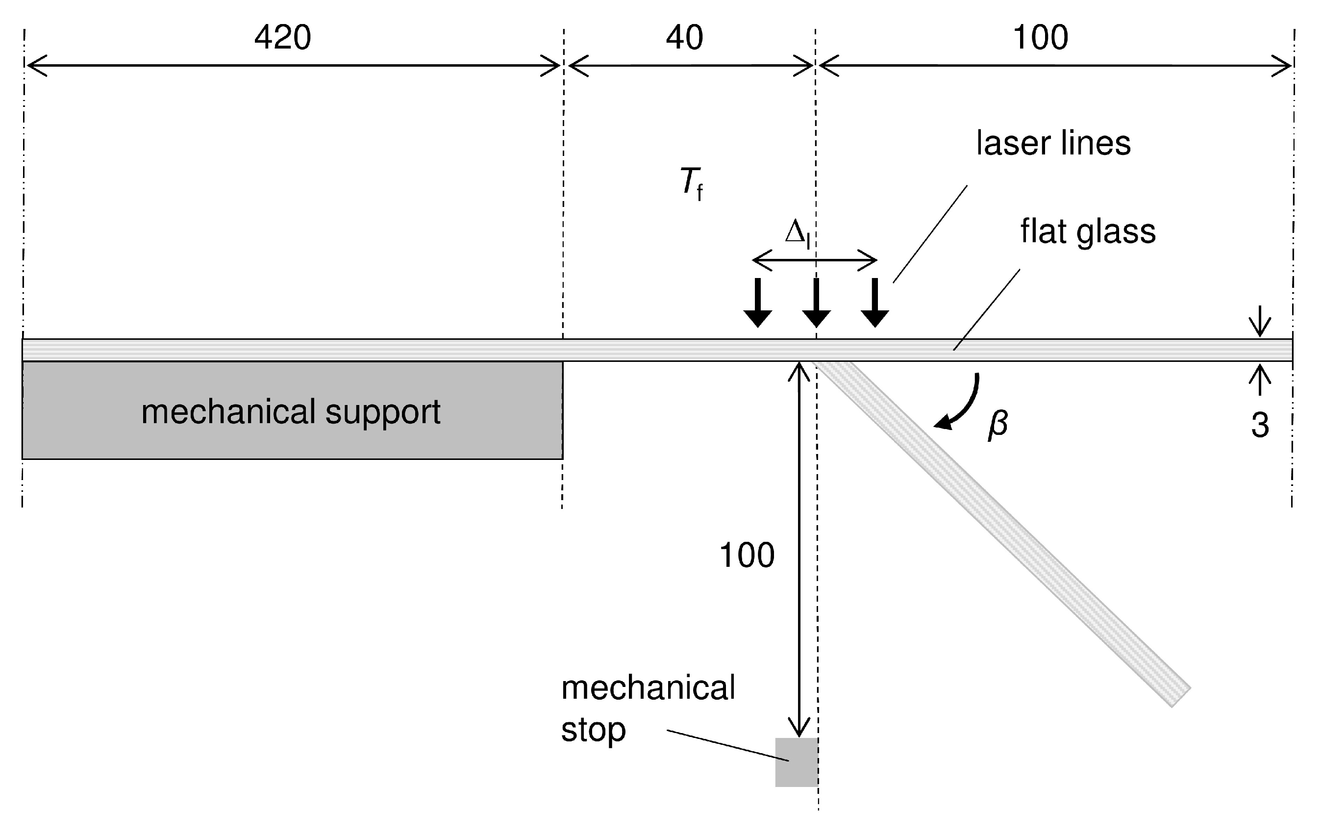
3.1. Laser Glass Bending

A first application example is laser glass bending. In the industrial standard process of glass bending [43], a flat glass specimen is placed in a furnace with furnace temperature T f , and then the heated specimen is bent at a designated edge driven by gravity. As an additional feature, a laser can be added to the industrial standard process in order to specifically heat up the critical region of the flat glass around the bending edge, and thus to speed up the process and achieve smaller bending radii [44,45]. The laser can generally scribe in arbitrary directions. In the process considered here, however, the laser path is restricted to three straight lines parallel to the bending edge. While the middle line defines the bending edge, the two outer lines are at a fixed distance Δ l / 2 = 5.75 mm in each direction to it. The laser spot moves along this path in multiple cycles with the number of cycles denoted by n c . The scribing speed and the power of the laser are kept constant. A mechanical stop below the bending edge guarantees that the bending angle does not exceed 90 ° . An illustration of the laser glass bending process is shown in Figure 1.
The goal of the glass bending process considered here is to obtain bent glass parts with a prescribed bending angle. In order to achieve such a pre-defined bending angle, the process operator has to find suitable combinations of the two process parameters T f and n c , which is usually done based on experience. A more systematic approach, however, is to set up an appropriate model of the bending angle y : = β as a function of the process variables
x : = ( x 1 , x 2 ) : = ( T f , n c ) X ,
where X R 2 is the rectangular set with the bounds specified in Table 1. In particular, such a model should allow sufficiently precise real-time predictions in order to support the process operator in quickly searching the parameter space X for optimal process parameter settings. Since SIAMOR models are polynomial by construction, they perfectly satisfy this real-time requirement. In contrast, a repeated evaluation of finite-element simulation models of the glass-bending process is too time-consuming to be of any practical use in quickly exploring the parameter space.
As generating experimental training data from the real process is cumbersome, a two-dimensional finite-element model was set up to generate data numerically. The simulation of the process was based on a coupled thermo-mechanical problem with finite deformation. Since the CO 2 laser used in the process operates in the opaque wavelength spectrum of glass, the heat supply was modeled as a surface flux into the deforming sheet. In this two-dimensional setting, the heat was assumed to be deposited instantaneously along the thickness direction and also instantaneously on all three laser lines. Radiation effects were ignored, and heat conduction inside the glass was described by the classical Fourier law with the heat conductivity obtained experimentally via laser flash analysis. In view of the relevant relaxation and process time scales for the applied temperature range, the mechanical behavior of the glass was described by a simple Maxwell-type visco-elastic law. The deformation due to gravity is heavily affected by the pronounced temperature dependence of the viscosity above the glass transition, which was described in our models using the Williams–Landel–Ferry approximation [46]. The generation of the simulated data was conducted using the commercial finite-element code Abaqus©. It was used to create a training dataset comprising 25 data points sampled on a 2D rectangular grid. The values used for the two degrees of freedom (five for T f and five for n c ) were placed equidistantly from the lower to the upper bounds given in Table 1.
Within these ranges and for the laser configuration described above, process experts expect the following monotonicity behavior: the bending angle y = β should increase monotonically with increasing glass temperature in the critical region, and thus with increasing T f and n c . In other words, the monotonicity signature σ of the bending angle y as a function of the inputs x from (15) is expected to be
σ = ( σ 1 , σ 2 ) = ( 1 , 1 ) .

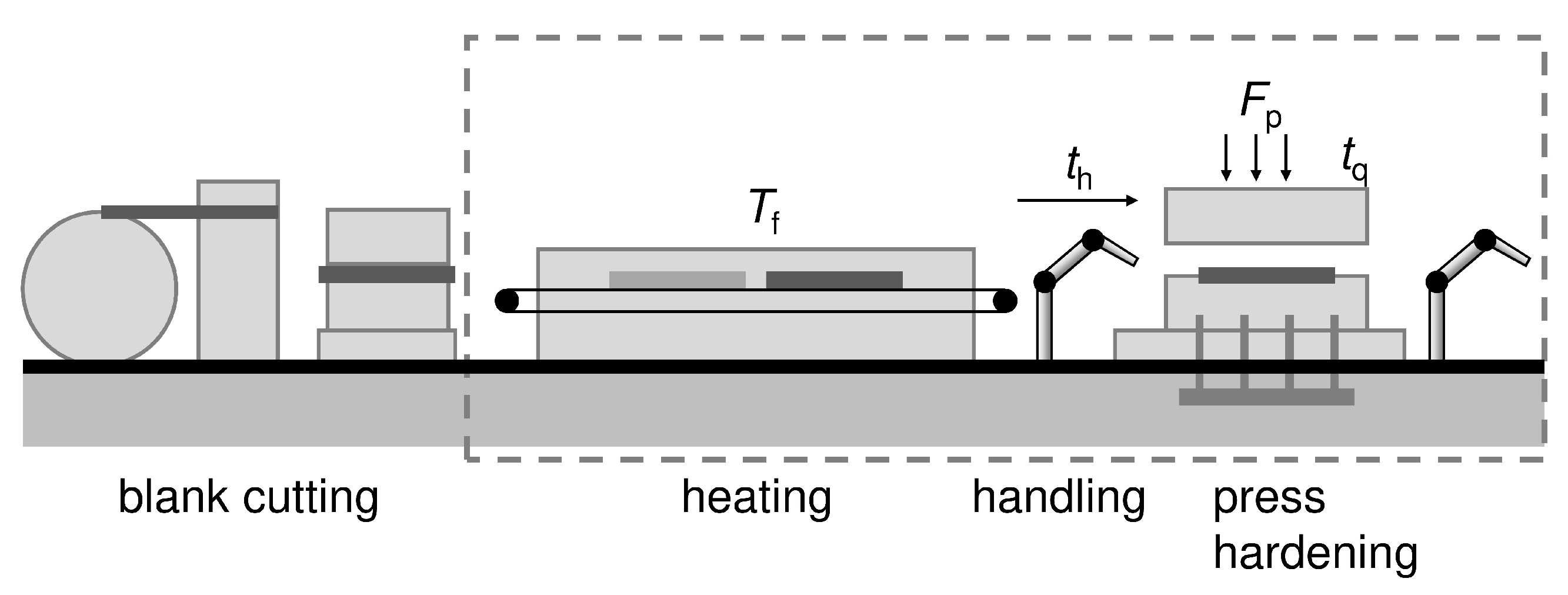
3.2. Forming and Press Hardening of Sheet Metal

Another application example is press hardening [47]. In the experimental setup considered here, a blank is placed in a chamber furnace with a furnace temperature T f above 900 ° C. After heating the blank, an industrial robot transports it with handling time t h into the cooled forming tool. In the following, the extra handling time Δ t h = t h 10 s is used instead, with 10 s being the minimum time the robot takes to move the blank from the furnace to the press. The final combined forming and quenching step allows for the variation of the press force F p and the quenching time t q . Afterwards, the formed part is transferred by the industrial robot to a deposition table for further cooling. An illustration of the process chain is shown in Figure 2.
The goal of the press hardening process considered in this work is to obtain a formed metal part with a prescribed hardness level, where the hardness is measured in units of the Vickers hardness number (unit symbol HV). In order to achieve such a pre-defined hardness, the process operator has to find suitable combinations of the four process parameters T f , Δ t h , F p , t q . And for that purpose, in turn, an appropriate model is needed for the hardness y of the formed part (at distinguished measurement points on the surface of the part) as a function of the process variables
x : = ( x 1 , , x 4 ) : = ( T f , Δ t h , F p , t q ) X ,
where X R 4 is the hypercuboid set with the bounds specified in Table 2. In particular, such a model has to allow sufficiently accurate real-time predictions in order to help the process operator in quickly searching the parameter space X for optimal process parameter settings. Since SIAMOR models are polynomial by construction, they perfectly satisfy this real-time requirement. In contrast, due to the four-dimensional parameter space, already a single evaluation of a representative finite-element simulation model of the press-hardening process is prohibitively time-consuming to be of any practical use in quickly exploring the parameter space.
As in the case of glass bending, experiments for the press hardening process are expensive because they usually require manual adjustments, which tend to be time-consuming. Additionally, the local hardness measurements at the chosen measurement points on the surface of the quenched part are time-consuming as well. This is why the training data base we used is rather small. It contains 60 points resulting from a design of experiments with the four process variables T f , Δ t h , F p and t q ranging between the bounds in Table 2, along with the corresponding hardness values at six local measurement points (referred to as MP1, …, MP6 in the following).
In order to compensate this data shortage, expert knowledge is brought into play. An expert for press hardening expects the hardness to decrease monotonically with Δ t h and to increase monotonically with T f as well as with t q . In other words, the monotonicity signature σ of the hardness y (at any given measurement point) as a function of the inputs x from (17) is expected to be
σ = ( σ 1 , , σ 4 ) = ( 1 , 1 , 0 , 1 ) .
In fact, a press hardening expert expects even a bit more, namely that the hardness should grow in a sigmoid-like manner with T f and that it grows concavely towards saturation with increasing t q . All these requirements result from qualitative physical considerations and are supported by empirical experience.

4. Results and Discussion

In this section, we describe the results of our semi-infinite adaptive optimization approach to monotonic regression (SIAMOR) in the industrial processes described in Section 3, and compare them to the results of other approaches to incorporating monotonicity knowledge, which are well-known from the literature.

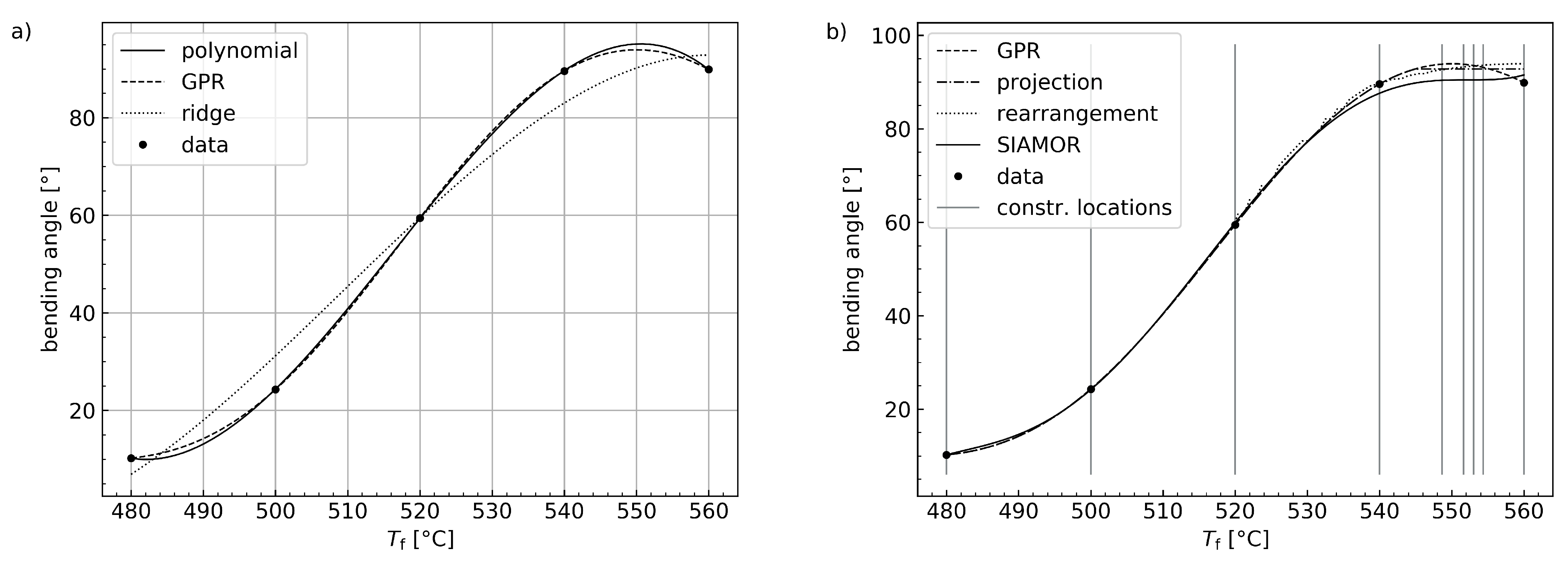
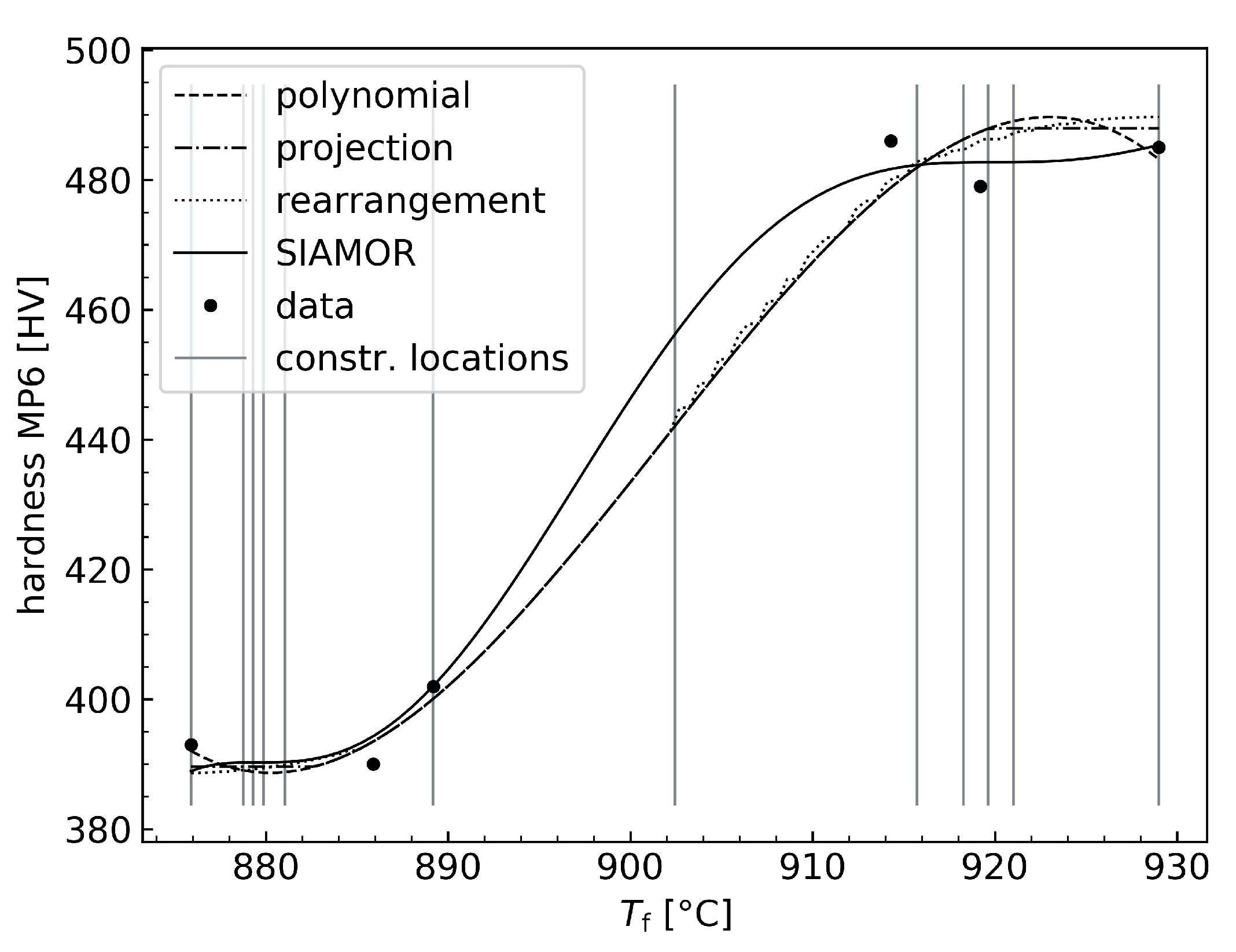
4.1. Informed Machine Learning Models for Laser Glass Bending

To begin with, the SIAMOR method was validated on a 1D subset of the data for laser glass bending, namely, the subset of all data points for which n c = 50 . This means that, out of the 25 data points, five points remained for training. First of all, ordinary unconstrained regression techniques were tried (see Figure 3a). A polynomial model of degree m = 3 (solid line) and a Gaussian process regressor [31] (GPR, dashed line) did not comply with the monotonicity knowledge at high T f . A radial basis function (RBF) kernel was used for the GPR. This non-parametric model is always a reasonable choice for simulated data because it accurately reproduces the data themselves if the noise-level parameter is kept small. For all GPR models in this work, that parameter was set to 10 5 . Next, the polynomial model was regularized in a ridge regression (dotted line), where the squared 2 -norm λ w 2 2 with a regularization weight λ was added to the objective function in (4). λ = 0.003 was chosen, which was roughly the minimum necessary value to achieve monotonicity. However, the resulting model does not predict the data very well. Thus, all three models from Figure 3a were unsatisfactory.
As a next step, the monotonicity requirement with respect to T f was brought to bear, and monotonic regression with the SIAMOR method ( m = 5 ) was used (see Figure 3b) and compared to the rearrangement [22] and to the monotonic projection [24] of the Gaussian process regressor from Figure 3a. As mentioned before, both comparative methods are based on a non-monotonic pre-trained reference predictor. This makes them fundamentally different to the SIAMOR method, which imposes the monotonicity already in the training phase. The projection was calculated as described in the Appendix A with | G | = 80 grid points. For the rearrangement method, the R package monreg was invoked from Python using the package rpy2. The degree m of the polynomial ansatz (1) used in the SIAMOR method was chosen as described in Section 2.3. For the specific case considered here, the curve started to vary unreasonably (albeit still monotonically) between the data points for m 6 , and therefore m = 5 was chosen. The SIAMOR algorithm was initialized with five equidistant constraint locations in X 0 , and it converged in iteration 5 with a total number of nine constraints. The locations of the constraints are marked in Figure 3b by the gray, vertical lines. The adaptive algorithm automatically places the non-initial constraints in the non-monotonic region at high T f . In terms of the root-mean-squared error
RMSE = 1 N l = 1 N y ^ ( x l ) t l 2
on the training data, the SIAMOR model fits the data best; see Table 3. Another advantage of the SIAMOR model is that it is continuously differentiable, whereas the rearrangement and projection models exhibit (slight) unphysical kinks, which are typical for these methods [22]. And finally, the rearrangement and the projection models, for temperatures higher than 540 ° C, both predict bending angles larger than 90 ° , which is unphysical due to the mechanical stop used in the glass bending process. In contrast, the predictions of the SIAMOR model do not (significantly) exceed 90 ° .
After these calculations on a 1D subset, the full 2D dataset of the considered laser glass bending process with its 25 data points was used. The results are shown in Figure 4. Again, part (a) of the figure displays an unconstrained Gaussian process regressor for comparison. The RBF kernel contained one length scale parameter per input dimension, and sklearn correctly adjusted these hyperparameters using L-BFGS-B. I.e., the employed length scales maximize the log-likelihood function of the model. Nevertheless, the model is unsatisfactory because it exhibits a bump in the rear right corner of the plot, contradicting the monotonicity knowledge.
Figure 4b shows the 2D monotonic projection of the GPR with the monotonicity requirements (16) with respect to T f and n c . It was calculated according to the Appendix A on a rectangular grid G consisting of 40 2 points (40 values per input dimension). The resulting model looks generally reasonable, and in particular, satisfies the monotonicity specifications, but it exhibits kinks and plateaus. The most conspicuous kink starts at about T f = 546 ° C, n c = 50 and proceeds towards the front right. The rearrangement method by [23] was not used for comparison here because for small datasets in d > 1 , it does not guarantee monotonicity.
Figure 4c displays the corresponding response surface of a polynomial model of the form (1) with degree m = 7 trained with SIAMOR. For m = 7 there are N m = 36 model parameters. The discretization X 0 was initialized with a rectangular grid using five equidistant values per dimension. The algorithm converged in iteration 11 with 69 final constraints. The resulting model is smoother than the one in Figure 4b, and it predicts the training data more accurately. Indeed, the corresponding RMSE values are 1.2518 ° for projection and 0.6607 ° for SIAMOR.

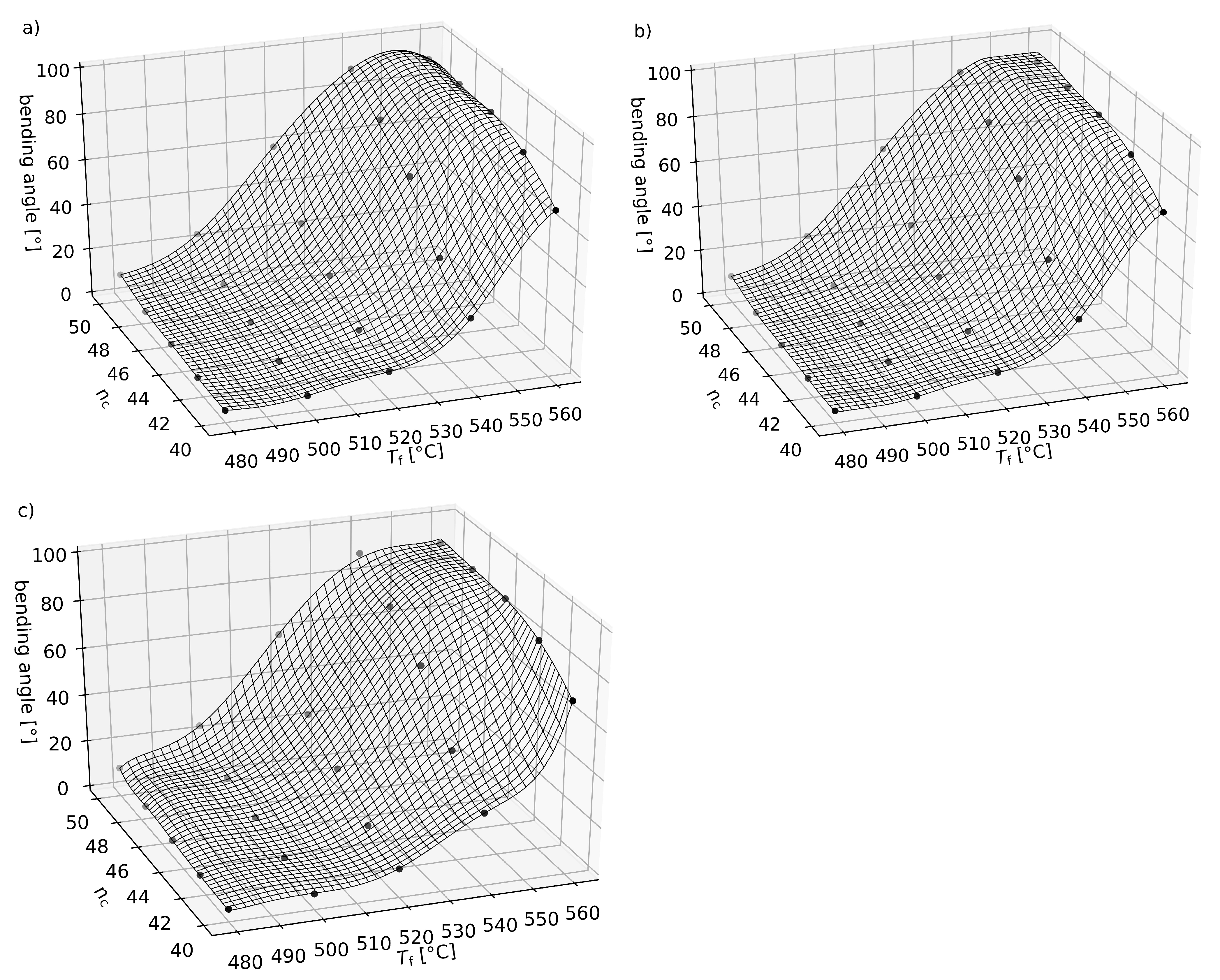
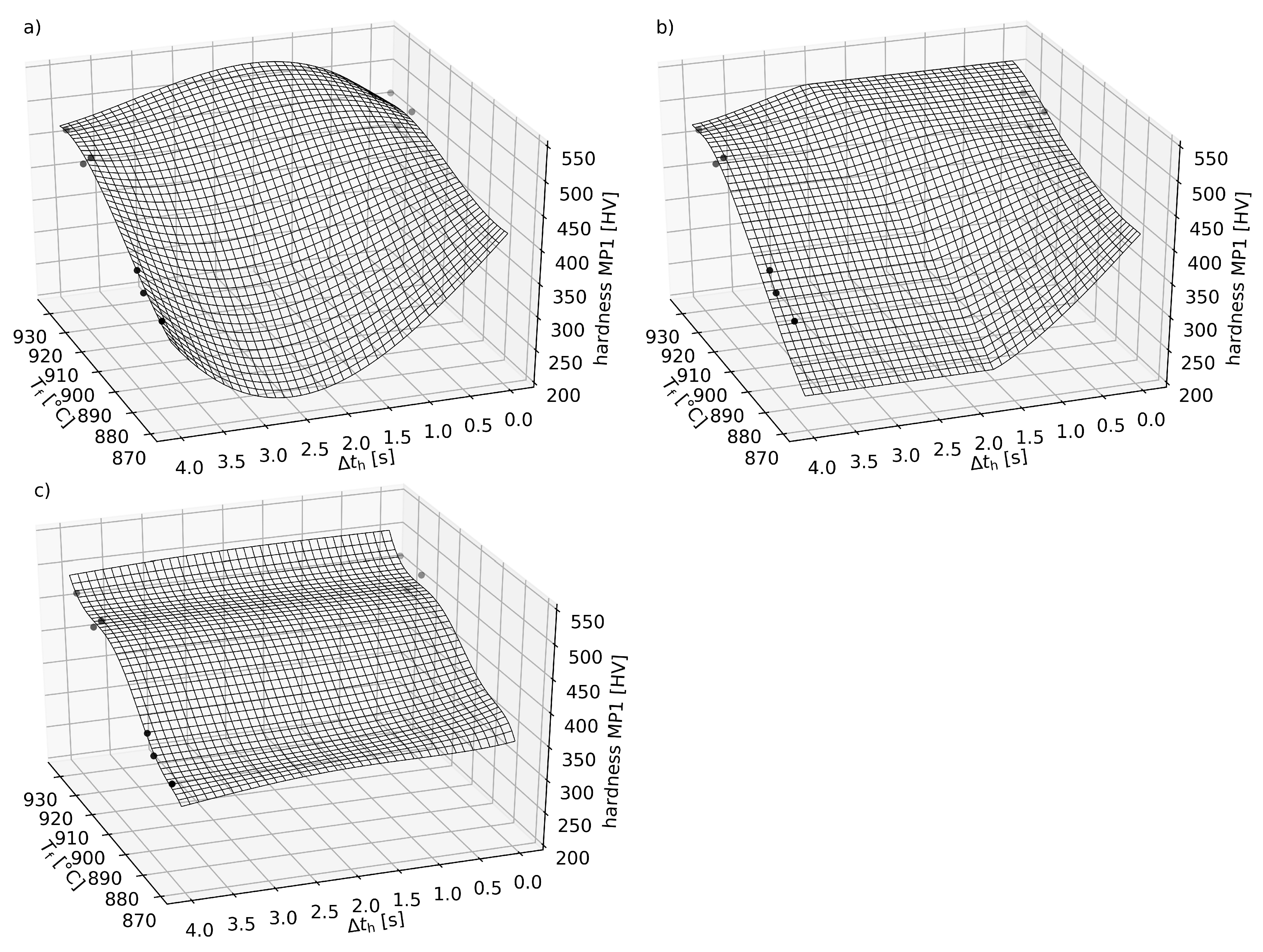
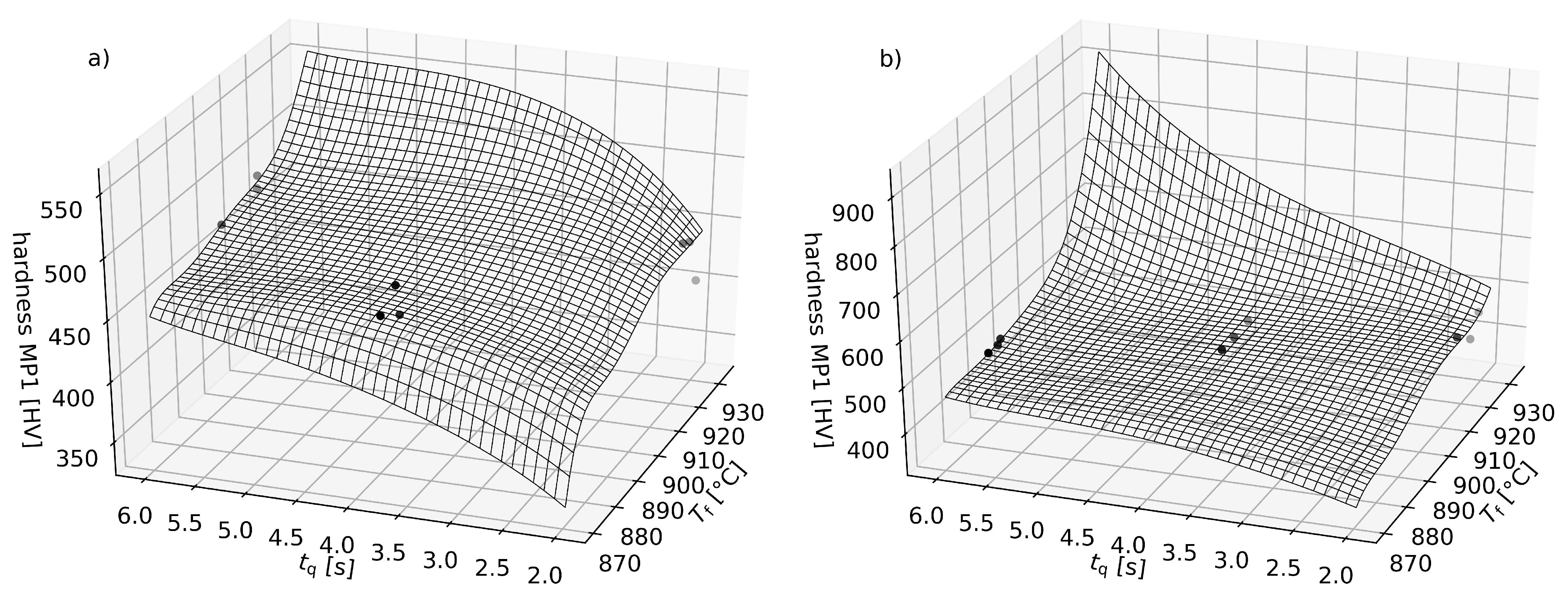
4.2. Informed Machine Learning Models for Forming and Press Hardening

As in the glass bending case, the SIAMOR method was first validated on a 1D subset of the data for the press hardening process. Namely, only those data points with F p = 2250 kN, Δ t h = 4 s and t q = 2 s were considered. These specifications are met by six data points, and these were used to train the models shown in Figure 5. The data are not monotonic due to experimental noise. However, they reflect the expected sigmoid-like behavior mentioned in Section 3.2, and this extends to the monotonized models. An unconstrained polynomial with m = 3 was chosen as the reference model to be monotonized for the comparative methods from the literature. Degrees lower than that resulted in larger deviations from the data and degrees higher than that resulted in overfitting. Thus, out of all models of the form (1), the hyperparameter choice m = 3 yielded the lowest RMSE values for projection and rearrangement. For the monotonic regression with SIAMOR, m = 6 and five equidistant initial constraint locations in X 0 were chosen. It converged in iteration 8 with a total of 12 monotonicity constraints. In terms of the root-mean-squared error, the SIAMOR model predicts the training data more accurately, as can be seen in Table 4. The reason is that the rearrangement- and projection-based models are dragged away from the data by the underlying reference model, especially at high T f .
After these 1D considerations, the SIAMOR method was validated on the full 4D dataset of the press hardening process. Polynomial models with degree m = 3 were used for unconstrained regression and monotonic projection, and polynomials with m = 6 were used for the SIAMOR method. The resulting models are visualized in the surface plots in Figure 6. The unconstrained model from Figure 6a clearly shows non-monotonic predictions with respect to Δ t h . Furthermore, the hardness slightly decreases with the furnace temperature at T f close to 930 ° C, which is not the behavior expected by the process expert either. Figure 6b shows the monotonic projection of the unconstrained model. It was computed according to the Appendix A on a grid G consisting of 40 4 points. The monotonic projection exhibits the kinks that are characteristic of that method, and it yields an RMSE of 28.84 HV on the entire dataset.
With an overall RMSE of 10.14 HV, the model resulting from SIAMOR is more accurate for this application. A corresponding response surface is displayed in Figure 6c. In keeping with (18), monotonicity was required with respect to T f (increasing), Δ t h (decreasing) and t q (increasing). As m = 6 , there are N m = 210 model parameters and the dicretization X 0 was initialized with a grid using four equidistant values per dimension. The algorithm converged in iteration 246 with 1372 final constraints. Our first try was with only two monotonicity requirements (namely, with respect to T f and t q ). We observed, however, that the final number of iterations decreased when the third monotonicity requirement was added. Thus, the monotonicity requirements in each direction promoted each other numerically within the algorithm and for the used data. This reduction in the number of iterations was not accompanied by a decrease in total calculation time because more lower-level problems have to be solved when there are more monotonicity directions.
With SIAMOR, monotonicity was achieved in all three input dimensions where it was required. See, e.g., Figure 6c, which is the monotonic counterpart of Figure 6a. A comparison of Figure 6a–c clearly shows how incorporating monotonicity expert knowledge helps compensate data shortages. Indeed, taking no monotonicity constraints into account at all (Figure 6a), we obtained an unexpected hardness minimum with respect to Δ t h at Δ t h 2.5 s and small T f . This also resulted in unnecessarily low predictions of the monotonic projection for small T f and Δ t h 1.5 s in Figure 6b. The SIAMOR model (Figure 6c), by contrast, predicted more reasonable hardness values in this range without needing additional data, because it integrated the available monotonicity knowledge in the training phase.
For the SIAMOR plots in Figure 7, Δ t h was reduced to 0 s. This figure shows that monotonicity is also achieved with respect to t q . Without having explicitly demanded it, the hardness y shows the expected concave growth towards saturation with respect to t q in Figure 7a. An additional increase in F p leads to Figure 7b, where the sign of the second derivative of y with respect to the quenching time t q changes along the T f -axis. I.e., the model changes its convexity properties in this direction and increases convexly instead of concavely with t q at high T f , Δ t h = 0 s and F p = 2250 kN. This contradicts the process expert’s expectations. A possible way out is to measure additional data (e.g., in the rear left corner of Figure 7b), which is elaborate and costly, however. Another possible way out is to add the concavity requirement x 4 2 y ^ w ( x ) 0 for all x X with respect to the x 4 = t q direction to the monotonicity constraints (6) used exclusively so far. In order to solve the resulting constrained regression problem, one can use the same adaptive semi-infinite solution strategy, which was already used for the monotonicity constraints alone.

5. Conclusions and Outlook

In this article, a proof of concept was conducted for the method of semi-infinite optimization with an adaptive discretization scheme to solve monotonic regression problems (SIAMOR). The method generates continuously differentiable models, and its use in multiple dimensions is straightforward. Polynomial models were used, but the method is not restricted to this type of model, even though it is numerically favorable because polynomial models lead to convex quadratic discretized problems. The monotonic regression technique was validated by means of two real-world applications from manufacturing. It resulted in predictions that complied very well with expert knowledge and that compensated for the lack of data to a certain extent. At least for the small datasets considered here, the resulting models predicted the training data more accurately than models based on the well-known projection or rearrangement methods from the literature.
While the present article is confined to regression under monotonicity constraints, semi-infinite optimization can also be exploited to treat other types of shape constraints such as concavity constraints, for instance. In fact, the shape constraints can be quite arbitrary, in principle. Additionally, this is only one of several aspects in the field of potential research on the method opened up by this work. Others are the testing of SIAMOR in combination with different model types, datasets or industrial processes. When using Gaussian process regressors instead of the polynomial models employed here, one can try out and compare various kernel types. Additionally, the SIAMOR method can be extended to locally varying monotonicity requirements (i.e., σ j = σ j ( x ) ).
Another possible direction of future research is to systematically investigate how to speed up the solution of the global lower-level problems. When more complex models or shape constraints are used, this will be particularly important. The solution of multiple lower-level problems and the final feasibility test on the reference grid can be parallelized to reduce the calculation time, for example. A rigorous investigation of the convergence properties and the asymptotic properties of the SIAMOR method and its possible generalizations is left to future research as well.

Author Contributions

Conceptualization, M.v.K., J.S. (Jochen Schmid), P.L. and A.S.; methodology, M.v.K., J.S. (Jochen Schmid) and J.S. (Jan Schwientek); software, M.v.K. and J.S. (Jochen Schmid); validation, M.v.K., J.S. (Jochen Schmid), P.L., R.Z., L.M., J.S. (Jan Schwientek) and A.S.; formal analysis, M.v.K., J.S. (Jochen Schmid) and J.S. (Jan Schwientek); investigation, M.v.K., J.S. (Jochen Schmid), P.L., R.Z., L.M. and A.S.; resources, P.L., L.M., I.S., T.K. and A.S.; data curation, P.L., L.M., I.S., T.K. and A.S.; writing—original draft preparation, M.v.K., J.S. (Jochen Schmid), P.L., R.Z. and I.S.; writing—review and editing, M.v.K., J.S. (Jochen Schmid), P.L., R.Z., L.M., I.S. and A.S.; visualization, M.v.K., P.L., R.Z. and L.M.; supervision, A.S. and T.K.; project administration, A.S. All authors have read and agreed to the published version of the manuscript.

Funding

This research was funded by the Fraunhofer Society within the lighthouse project “Machine Learning for Production” (ML4P).

Institutional Review Board Statement

Not applicable.

Informed Consent Statement

Not applicable.

Data Availability Statement

Not available.

Acknowledgments

We would like to thank Michael Bortz and Raoul Heese for valuable discussions about integrating expert knowledge into machine learning models. We also gratefully acknowledge funding from the Fraunhofer Society within the lighthouse project “Machine Learning for Production” (ML4P). And finally, we would like to thank the anonymous reviewers for their valuable comments.

Conflicts of Interest

The authors declare no conflict of interest.

Abbreviations

The following abbreviations are used in this manuscript:
SIAMORSemi-infinite optimization approach to monotonic regression
GPRGaussian process regression
RBFRadial basis function
RMSERoot mean squared error

Appendix A. Computing Monotonic Projections

In order to validate our semi-infinite optimization approach to monotonic regression, it is compared, among other things, to the projection-based monotonization approach by [24]. As has been pointed out in Section 1, the projection method starts out from a purely data-based initial model y ^ 0 (a Gaussian process regressor in the case of [24]) and then replaces this initial model by the monotonic projection y ^ of y ^ 0 . I.e., y ^ : X R is the monotonic square-integrable function with monotonicity signature σ that is closest to y ^ 0 in the L 2 -norm.
In order to numerically compute this monotonic projection y ^ , the original procedure proposed in [24] is not used here, though. Instead, the conceptually and computationally simpler methodology from [48] is employed. In this methodology, the input space X is discretized with a fine rectangular grid G. Then, the corresponding discrete monotonic projection ( y ^ ( x ) ) x G , that is, the solution of the constrained optimization problem
min z R G x G z ( x ) y ^ 0 ( x ) 2 s . t . σ j · z ( x + h j e j ) z ( x ) 0 for all j J and all x G for which x + h j e j G
is computed. In the above relation, R G is the | G | -dimensional vector space of all R -valued functions z = ( z ( x ) ) x G defined on the discrete set G, h j > 0 indicates the distance of adjacent grid points in the jth coordinate direction, and e j R d is the jth canonical unit vector. It is shown in [48] that the extension of ( y ^ ( x ) ) x G to a grid-constant function on the whole of X is a good approximation of the monotonic projection y ^ , if only the grid is fine enough and the initial model y ^ 0 is continuous, for instance. In contrast to [24], these approximation results from [48] also feature rates of convergence.
Since both the objective function and the constraints of (A1) are convex with respect to z, the problem (A1) is a convex program. We used cvxopt [49] to solve these problems because it offers a sparse matrix type to represent the large coefficient and constraint matrices for d > 1 . Alternatively, the discrete monotonic projection problems can also be solved using any of the more sophisticated computational methods from ([50], Section 2.3), ([51], Section 4.1), or [52,53,54,55,56]. However, for the number of input dimensions considered here, our direct computational method is sufficient.

References

  1. Weichert, D.; Link, P.; Stoll, A.; Rüping, S.; Ihlenfeldt, S.; Wrobel, S. A review of machine learning for the optimization of production processes. Int. J. Adv. Manuf. Technol. 2019, 104, 1889–1902. [Google Scholar] [CrossRef]
  2. MacInnes, J.; Santosa, S.; Wright, W. Visual classification: Expert knowledge guides machine learning. IEEE Comput. Graph. Appl. 2010, 30, 8–14. [Google Scholar] [CrossRef]
  3. Heese, R.; Walczak, M.; Morand, L.; Helm, D.; Bortz, M. The Good, the Bad and the Ugly: Augmenting a Black-Box Model with Expert Knowledge. In Artificial Neural Networks and Machine Learning—ICANN 2019: Workshop and Special Sessions; Lecture Notes in Computer, Science; Tetko, I.V., Kůrková, V., Karpov, P., Theis, F., Eds.; Springer International Publishing: Cham, Switzerland, 2019; Volume 11731, pp. 391–395. [Google Scholar] [CrossRef] [Green Version]
  4. Rueden, L.V.; Mayer, S.; Beckh, K.; Georgiev, B.; Giesselbach, S.; Heese, R.; Kirsch, B.; Pfrommer, J.; Pick, A.; Ramamurthy, R.; et al. Informed Machine Learning—A Taxonomy and Survey of Integrating Knowledge into Learning Systems. IEEE Trans. Knowl. Data Eng. 2021. [Google Scholar] [CrossRef]
  5. Johansen, T.A. Identification of non-linear systems using empirical data and prior knowledge—An optimization approach. Automatica 1996, 32, 337–356. [Google Scholar] [CrossRef]
  6. Mangasarian, O.L.; Wild, E.W. Nonlinear knowledge in kernel approximation. IEEE Trans. Neural Netw. 2007, 18, 300–306. [Google Scholar] [CrossRef] [Green Version]
  7. Mangasarian, O.L.; Wild, E.W. Nonlinear knowledge-based classification. IEEE Trans. Neural Netw. 2008, 19, 1826–1832. [Google Scholar] [CrossRef] [PubMed] [Green Version]
  8. Cozad, A.; Sahinidis, N.V.; Miller, D.C. A combined first-principles and data-driven approach to model building. Comput. Chem. Eng. 2015, 73, 116–127. [Google Scholar] [CrossRef]
  9. Wilson, Z.T.; Sahinidis, N.V. The ALAMO approach to machine learning. Comput. Chem. Eng. 2017, 106, 785–795. [Google Scholar] [CrossRef] [Green Version]
  10. Wilson, Z.T.; Sahinidis, N.V. Automated learning of chemical reaction networks. Comput. Chem. Eng. 2019, 127, 88–98. [Google Scholar] [CrossRef]
  11. Asprion, N.; Böttcher, R.; Pack, R.; Stavrou, M.E.; Höller, J.; Schwientek, J.; Bortz, M. Gray-Box Modeling for the Optimization of Chemical Processes. Chem. Ing. Tech. 2019, 91, 305–313. [Google Scholar] [CrossRef]
  12. Heese, R.; Nies, J.; Bortz, M. Some Aspects of Combining Data and Models in Process Engineering. Chem. Ing. Tech. 2020, 92, 856–866. [Google Scholar] [CrossRef] [Green Version]
  13. Altendorf, E.E.; Restificar, A.C.; Dietterich, T.G. Learning from Sparse Data by Exploiting Monotonicity Constraints. In Proceedings of the Twenty-First Conference on Uncertainty in Artificial Intelligence, UAI’05, Edinburgh, UK,, 26–29 July 2005; AUAI Press: Arlington, VA, USA, 2005; pp. 18–26. [Google Scholar]
  14. Kotłowski, W.; Słowiński, R. Rule learning with monotonicity constraints. In Proceedings of the 26th Annual International Conference on Machine Learning—ICML’09, Montreal, QC, Canada, 14–18 June 2009; Danyluk, A., Bottou, L., Littman, M., Eds.; ACM Press: New York, NY, USA, 2009; pp. 1–8. [Google Scholar]
  15. Lauer, F.; Bloch, G. Incorporating prior knowledge in support vector machines for classification: A review. Neurocomputing 2008, 71, 1578–1594. [Google Scholar] [CrossRef] [Green Version]
  16. Groeneboom, P.; Jongbloed, G. Nonparametric Estimation under Shape Constraints; Cambridge University Press: Cambridge, UK, 2014. [Google Scholar] [CrossRef]
  17. Gupta, M.; Cotter, A.; Pfeifer, J.; Voevodski, K.; Canini, K.; Mangylov, A.; Moczydlowski, W.; van Esbroeck, A. Monotonic Calibrated Interpolated Look-Up Tables. J. Mach. Learn. Res. (JMLR) 2016, 17, 1–47. [Google Scholar]
  18. Mukerjee, H. Monotone Nonparametric Regression. Ann. Stat. 1988, 16, 741–750. [Google Scholar] [CrossRef]
  19. Mammen, E. Estimating a smooth monotone regression function. Ann. Stat. 1991, 19, 724–740. [Google Scholar] [CrossRef]
  20. Mammen, E.; Marron, J.S.; Turlach, B.A.; Wand, M.P. A General Projection Framework for Constrained Smoothing. Stat. Sci. 2001, 16, 232–248. [Google Scholar] [CrossRef]
  21. Hall, P.; Huang, L.S. Nonparametric kernel regression subject to monotonicity constraints. Ann. Stat. 2001, 29, 624–647. [Google Scholar] [CrossRef]
  22. Dette, H.; Neumeyer, N.; Pilz, K.F. A simple nonparametric estimator of a strictly monotone regression function. Bernoulli 2006, 12, 469–490. [Google Scholar] [CrossRef]
  23. Dette, H.; Scheder, R. Strictly monotone and smooth nonparametric regression for two or more variables. Can. J. Stat. 2006, 34, 535–561. [Google Scholar] [CrossRef] [Green Version]
  24. Lin, L.; Dunson, D.B. Bayesian monotone regression using Gaussian process projection. Biometrika 2014, 101, 303–317. [Google Scholar] [CrossRef] [Green Version]
  25. Chernozhukov, V.; Fernandez-Val, I.; Galichon, A. Improving point and interval estimators of monotone functions by rearrangement. Biometrika 2009, 96, 559–575. [Google Scholar] [CrossRef] [Green Version]
  26. Lauer, F.; Bloch, G. Incorporating prior knowledge in support vector regression. Mach. Learn. 2007, 70, 89–118. [Google Scholar] [CrossRef] [Green Version]
  27. Chuang, H.C.; Chen, C.C.; Li, S.T. Incorporating monotonic domain knowledge in support vector learning for data mining regression problems. Neural Comput. Appl. 2020, 32, 11791–11805. [Google Scholar] [CrossRef]
  28. Riihimäki, J.; Vehtari, A. Gaussian processes with monotonicity information. Proc. Mach. Learn. Res. 2010, 9, 645–652. [Google Scholar]
  29. Neumann, K.; Rolf, M.; Steil, J.J. Reliable integration of continuous constraints into extreme learning machines. Int. J. Uncertain. Fuzziness Knowl.-Based Syst. 2013, 21, 35–50. [Google Scholar] [CrossRef] [Green Version]
  30. Friedlander, F.G.; Joshi, M.S. Introduction to the Theory of Distributions, 2nd ed.; Cambridge University Press: Cambridge, UK, 1998. [Google Scholar]
  31. Rasmussen, C.E.; Williams, C.K.I. Gaussian Processes for Machine Learning; Adaptive Computation and Machine Learning; MIT: Cambridge, MA, USA; London, UK, 2006. [Google Scholar]
  32. Hettich, R.; Zencke, P. Numerische Methoden der Approximation und Semi-Infiniten Optimierung; Teubner Studienbücher: Mathematik; Teubner: Stuttgart, Germany, 1982. [Google Scholar]
  33. Polak, E. Optimization: Algorithms and Consistent Approximations; Applied Mathematical Sciences; Springer: New York, NY, USA; London, UK, 1997; Volume 124. [Google Scholar]
  34. Reemtsen, R.; Rückmann, J.J. Semi-Infinite Programming; Nonconvex Optimization and Its Applications; Kluwer Academic: Boston, MA, USA; London, UK, 1998; Volume 25. [Google Scholar]
  35. Stein, O. Bi-Level Strategies in Semi-Infinite Programming; Nonconvex Optimization and Its Applications; Kluwer Academic: Boston, MA, USA; London, UK, 2003; Volume 71. [Google Scholar]
  36. Stein, O. How to solve a semi-infinite optimization problem. Eur. J. Oper. Res. 2012, 223, 312–320. [Google Scholar] [CrossRef]
  37. Shimizu, K.; Ishizuka, Y.; Bard, J.F. Nondifferentiable and Two-Level Mathematical Programming; Kluwer Academic Publishers: Boston, MA, USA; London, UK, 1997. [Google Scholar]
  38. Dempe, S.; Kalashnikov, V.; Pérez-Valdés, G.A.; Kalashnykova, N. Bilevel Programming Problems; Springer: Berlin/Heidelberg, Germany, 2015. [Google Scholar] [CrossRef]
  39. Blankenship, J.W.; Falk, J.E. Infinitely constrained optimization problems. J. Optim. Theory Appl. 1976, 19, 261–281. [Google Scholar] [CrossRef]
  40. Nocedal, J.; Wright, S.J. Numerical Optimization, 2nd ed.; Springer Series in Operations Research; Springer: New York, NY, USA, 2006. [Google Scholar]
  41. Goldfarb, D.; Idnani, A. A numerically stable dual method for solving strictly convex quadratic programs. Math. Program. 1983, 27, 1–33. [Google Scholar] [CrossRef]
  42. Endres, S.C.; Sandrock, C.; Focke, W.W. A simplicial homology algorithm for Lipschitz optimisation. J. Glob. Optim. 2018, 72, 181–217. [Google Scholar] [CrossRef] [Green Version]
  43. Neugebauer, J. Applications for curved glass in buildings. J. Facade Des. Eng. 2014, 2, 67–83. [Google Scholar] [CrossRef] [Green Version]
  44. Rist, T.; Gremmelspacher, M.; Baab, A. Feasibility of bent glasses with small bending radii. CE/Papers 2018, 2, 183–189. [Google Scholar] [CrossRef]
  45. Rist, T.; Gremmelspacher, M.; Baab, A. Innovative Glass Bending Technology for Manufacturing Expressive Shaped Glasses with Sharp Curves. Glass Performance Days. 2019, pp. 34–35. Available online: https://www.glassonweb.com/article/innovative-glass-bending-technology-manufacturing-expressive-shaped-glasses-with-sharp (accessed on 26 November 2021).
  46. Williams, M.L.; Landel, R.F.; Ferry, J.D. The Temperature Dependence of Relaxation Mechanisms in Amorphous Polymers and Other Glass-forming Liquids. J. Am. Chem. Soc. 1955, 77, 3701–3707. [Google Scholar] [CrossRef]
  47. Neugebauer, R.; Schieck, F.; Polster, S.; Mosel, A.; Rautenstrauch, A.; Schönherr, J.; Pierschel, N. Press hardening—An innovative and challenging technology. Arch. Civ. Mech. Eng. 2012, 12, 113–118. [Google Scholar] [CrossRef]
  48. Schmid, J. Approximation, characterization, and continuity of multivariate monotonic regression functions. Anal. Appl. 2021. [Google Scholar] [CrossRef]
  49. Andersen, M.; Dahl, J.; Liu, Z.; Vandenberghe, L. Interior-point methods for large-scale cone programming. In Optimization for Machine Learning; Sra, S., Nowozin, S., Wright, S.J., Eds.; MIT Press: Cambridge, MA, USA, 2011; pp. 55–83. [Google Scholar]
  50. Barlow, R.E. Statistical Inference under Order Restrictions: The Theory and Application of Isotonic Regression; Wiley Series in Probability and Mathematical Statistics; Wiley: London, UK; New York, NY, USA, 1972; Volume 8. [Google Scholar]
  51. Robertson, T.; Wright, F.T.; Dykstra, R. Statistical Inference under Inequality Constraints; Wiley Series in Probability and Mathematical Statistics. Probability and Mathematical Statistics Section; Wiley: Chichester, UK; New York, NY, USA, 1988. [Google Scholar]
  52. Qian, S.; Eddy, W.F. An Algorithm for Isotonic Regression on Ordered Rectangular Grids. J. Comput. Graph. Stat. 1996, 5, 225–235. [Google Scholar] [CrossRef]
  53. Spouge, J.; Wan, H.; Wilbur, W.J. Least Squares Isotonic Regression in Two Dimensions. J. Optim. Theory Appl. 2003, 117, 585–605. [Google Scholar] [CrossRef]
  54. Stout, Q.F. Isotonic Regression via Partitioning. Algorithmica 2013, 66, 93–112. [Google Scholar] [CrossRef] [Green Version]
  55. Stout, Q.F. Isotonic Regression for Multiple Independent Variables. Algorithmica 2015, 71, 450–470. [Google Scholar] [CrossRef] [Green Version]
  56. Kyng, R.; Rao, A.; Sachdeva, S. Fast, Provable Algorithms for Isotonic Regression in all lp-norms. In Advances in Neural Information Processing Systems 28; Cortes, C., Lawrence, N.D., Lee, D.D., Sugiyama, M., Garnett, R., Eds.; Curran Associates, Inc.: New York, NY, USA, 2015; pp. 2719–2727. [Google Scholar]
Figure 1. Side view of the laser glass bending process. Symbols: T f —furnace temperature, Δ l —distance between the left- and right-most laser line, β —bending angle. Lengths are given in mm.
Algorithms 14 00345 g001
Figure 2. Side view of the press hardening process [47] indicating the considered process steps. Symbols: T f —furnace temperature, t h —handling time, F p —press force, t q —quenching time.
Algorithms 14 00345 g002
Figure 3. 1D regression for laser glass bending ( n c = 50 ). (a) Unconstrained regression. Solid: polynomial model ( m = 3 ), dashed: Gaussian process regression (GPR) with RBF kernel (noise level 10 5 ), dotted: polynomial ridge regression ( m = 3 , λ = 0.003 ). (b) Monotonic regression, with the solid line resulting from the SIAMOR method (see Section 2.1, Section 2.2 and Section 2.3) with degree m = 5 . The projection [24] (dash-dotted) and rearrangement [22] (dotted) methods were fed with the dashed GPR curve as a non-monotonic reference predictor.
Algorithms 14 00345 g003
Figure 4. 2D regression for laser glass bending, where the markers represent the employed training data. (a) Gaussian process regression (non-monotonic) with a multi-length-scale RBF kernel (noise level 10 5 ); (b) projection [24] of GPR; (c) monotonic regression of a polynomial model ( m = 7 ) using the SIAMOR method (see Section 2.1, Section 2.2 and Section 2.3).
Algorithms 14 00345 g004
Figure 5. 1D regression for forming and press hardening of sheet metal ( F p = 2250 kN, Δ t h = 4 s, t q = 2 s). Dashed: (non-monotonic) polynomial of degree m = 3 as the reference model, dash-dotted: projection [24], dotted: rearrangement [22], solid: SIAMOR (see Section 2.1, Section 2.2 and Section 2.3) with degree m = 6 . The projection and rearrangement methods were fed with the dashed polynomial curve as non-monotonic reference predictor.
Algorithms 14 00345 g005
Figure 6. 4D regression for forming and press hardening of sheet metal using polynomial models ( F p = 2250 kN, t q = 2 s). The markers represent those training points matching the specification of the corresponding plane in the input space. (a) Unconstrained m = 3 , (b) projection [24] of unconstrained m = 3 , (c) SIAMOR m = 6 .
Algorithms 14 00345 g006
Figure 7. Response surfaces of 4D monotonic regression with SIAMOR ( m = 6 ) for forming and press hardening of sheet metal ( Δ t h = 0 s). The markers represent those training points matching the specifications of the corresponding planes in the input space. (a) F p = 1750 kN, (b) F p = 2250 kN.
Algorithms 14 00345 g007
Table 1. Ranges for the process variables of laser glass bending.
VariableMinMaxPhys. Unit
T f 480560 ° C
n c 4050
Table 2. Ranges for the process variables of press hardening.
VariableMinMaxPhys. Unit
T f 871933 ° C
Δ t h 04s
F p 17502250kN
t q 26s
Table 3. Root-mean-squared deviations (RMSE) of the monotonic regression models from the training data for laser glass bending (1D).
Monotonic Regression TypeRMSE [ ° ]
projection [24]         1.3822
rearrangement [22]         1.8432
SIAMOR         1.1598
Table 4. Root-mean-squared deviations (RMSE) of the monotonic regression models from the training data for forming and press hardening of sheet metal (1D).
Monotonic Regression TypeRMSE [HV]
projection [24]         5.0893
rearrangement [22]         4.8346
SIAMOR         3.3583
Publisher’s Note: MDPI stays neutral with regard to jurisdictional claims in published maps and institutional affiliations.

