The Buy-Online-Pick-Up-in-Store Retailing Model: Optimization Strategies for In-Store Picking and Packing

Abstract

Online shopping is growing fast due to the increasingly widespread use of digital services. During the COVID-19 pandemic, the desire for contactless shopping has further changed consumer behavior and accelerated the acceptance of online grocery purchases. Consequently, traditional brick-and-mortar retailers are developing omnichannel solutions such as click-and-collect services to fulfill the increasing demand. In this work, we consider the Buy-Online-Pick-up-in-Store concept, in which online orders are collected by employees of the conventional stores. As labor is a major cost driver, we apply and discuss different optimizing strategies in the picking and packing process based on real-world data from a German retailer. With comparison of different methods, we estimate the improvements in efficiency in terms of time spent during the picking process. Additionally, the time spent on the packing process can be further decreased by applying a mathematical model that guides the employees on how to organize the articles in different shopping bags during the picking process. In general, we put forward effective strategies for the Buy-Online-Pick-up-in-Store paradigm that can be easily implemented by stores with different topologies.

1. Introduction

Online shopping has become popular with the development of digitization over the past decade [1]. With the restrictions and social distancing imposed during the first and second wave of the COVID-19 pandemic, an increasing number of people explored online purchasing for groceries for the first time. In this context, traditional brick-and-mortar retailers were offered an opportunity to build or improve omnichannel solutions for their businesses [2].

Among different ways to design an omnichannel model [2,3], a straightforward and widely used method is utilizing the already existing brick-and-mortar structures for both regular walk-in customers and online order fulfillment [4]. The focus of this work is based on this paradigm, referred to as the Buy-Online-Pick-up-in-Store concept (BOPS). It allows an effective mixed online–offline business model transition with the least amount of time and financial resource investments required.

Due to the fact that this is a relatively new topic, the existing literature is limited. A literature search revealed that the majority of the focus is on marketing and management aspects such as service area [5], pricing strategy [6], and inventory levels [7], while operational optimization is rarely mentioned. As a result, it is not surprising that the retailer providing data for this study had little to no optimization in place for the BOPS in-store operations: the employees receive shopping lists in a random order, they go through the store similar to regular customers to pick up all the items, and then go to the cashier to scan the products and place them in the final bags. Following this description, two major issues emerge: the non-optimized picking path, which has a longer travel time, and the need to pass through the cashier, both of which result in an inefficient use of the available human resources.

In this work, we discuss different optimization methods to solve these major issues in terms of the picking and packing process, and we propose a comprehensive optimization strategy that reduces the overall human resource time required and guarantees the quality of packaging to prevent potential damage.

The remainder of this work is structured as follows: in Section 2 the existing literature related to the topics addressed in this research is reviewed. In Section 3, we optimize the picking process in the BOPS model with different routing analyses. In Section 4, a two-step optimization, which improves packing efficiency by calculating the minimum number of bags needed for a shopping list and balances the volume and weight of the products packed in the available bags, is discussed. As the picking time performance improved when both optimizations were implemented, experimental simulation on fully optimized shopping lists was performed in Section 6. A summary of the accomplishments of the work and further discussions are finally presented in Section 7.

2. Literature Review

With the growing amount of interest in the topic of Buy-Online-Pick-up-in-Store, the majority of the research up to this point has focused on the effects that launching a BOPS channel would have on the previously existing store. For example, one work [8] investigates how inventory holding costs and lost sales costs are influenced by giving walk-in customers a higher priority than BOPS customers, and how this influence varies depending on whether the BOPS is owned by the shop or by a third party. The work [9] analyzes a Stackelberg game theoretic model involving a manufacturer and a retailer to determine how shop prices should fluctuate in response to the manufacturer’s product quality and which scenarios are profitable. There is plenty of research [5,6,7,10,11,12], which is helpful in determining if it is beneficial to open the BOPS channel and start planning for a well-functioning business model, but they provide no guidance on how operations should be organized, which is vital for the long term success of the BOPS channel.

When the search is expanded to include similar topics, a ship-from-store concept is studied in [13]: in both the concept and the BOPS model, customers place orders via an application or a website and employees go through the store to pick the products. The authors propose a model to determine the optimal time to batch multiple orders before the picking operation is started, the optimal time before starting the delivery process of orders, and the optimal number of pickers and packers. However, this model is not very practical in grocery stores, as the batching/reassembling operations applied to the problem would significantly increase the complexity of the task due to the high number of items on shopping lists, thus implementation of this strategy is not recommended in the scenario of this BOPS research. Similarly in [14], a methodology is proposed to compute the minimal picking rate under single wave or multi wave picking given a demand ordered between two cutoff times and an objective service level. The picking operation is not modeled, but they assume that there exists a certain picking rate $\mu$ to be defined before the proposed model can be used to validate strategies. A research gap can therefore be identified, given the fact that in the literature no approach optimizing grocery store order picking in a BOPS system was found.

Order picking in warehouses is a well examined topic, with an extensive body of work investigating routing, storage, and batch assignment that aims at optimizing and automatizing costly operations [15]. These approaches can not however be utilized in the BOPS contexts, due to the differences in terms of layout, means of transport, and stored units. In fact, while in warehouses one can use robots for moving Unit Load Devices or place the most frequently picked items in easy to reach spots, in brick-and-mortar stores the presence of regular customers and the different packaging shapes makes the implementation of robots almost impossible. Since the design methodology of the stores is selling products, the main factors taken into account are revenue maximization [4] and customer satisfaction [16]. This is accomplished by having a good variety, visibility, and availability of products positioned in strategic ways that increase impulsive purchases, but has no correlation with an employee who picks the articles according to a given shopping list.

From the customers’ perspective, the in-store picking problem has been discussed in [17]. By analyzing customers’ locations detected through devices on the shopping carts, the paper revealed that customers whose path was closer to the shortest path tended to buy items from frequently purchased product categories with higher numbers of products. Larger shopping baskets lead to higher deviations from the optimal path, and most deviations are not caused by not following the optimal zone order but by not taking the shortest route between them. However, if an employee is given an optimized shopping list to pick up all the items, he/she can take the shortest route following the optimal zone order to improve efficiency. In the work [18], they propose solving the in-store picking problem as an open Traveling Salesman Problem (TSP) on an underlying graph representing the location of the items within the shop. This resulted in a significant increase in performance by picking time.

Considering that in-store logistics are typically handled by people and labor is a major cost-driver, such an approach makes sense in the BOPS context. However, the peculiar item disposition can lead to potential product damaging, since product attributes such as mass, size and fragility are not taken into account when designing the layout [4,16] or optimizing the picking route as a TSP. Therefore, constraints regarding the features of the articles are taken into account in [19] and the problem is solved as a Sequential Ordering Problem [20].

The packing problem in a retail context in the BOPS model has not been addressed in the literature thus far. An inspiring point to this work is the bin packing problem [21] or 3D bin packing problem [22], which is usually used for the design of item positioning on unit load devices such as containers and pallets.

3. The Picking Problem

3.1. Problem Statement

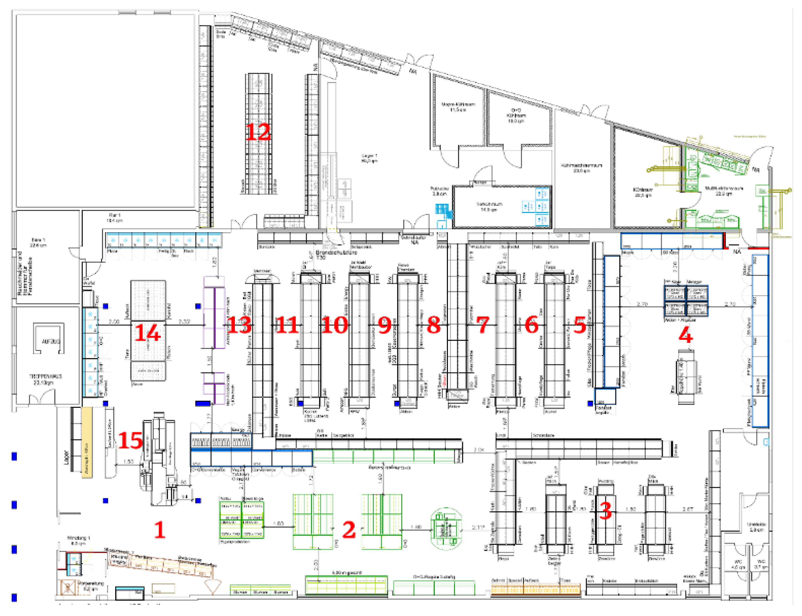
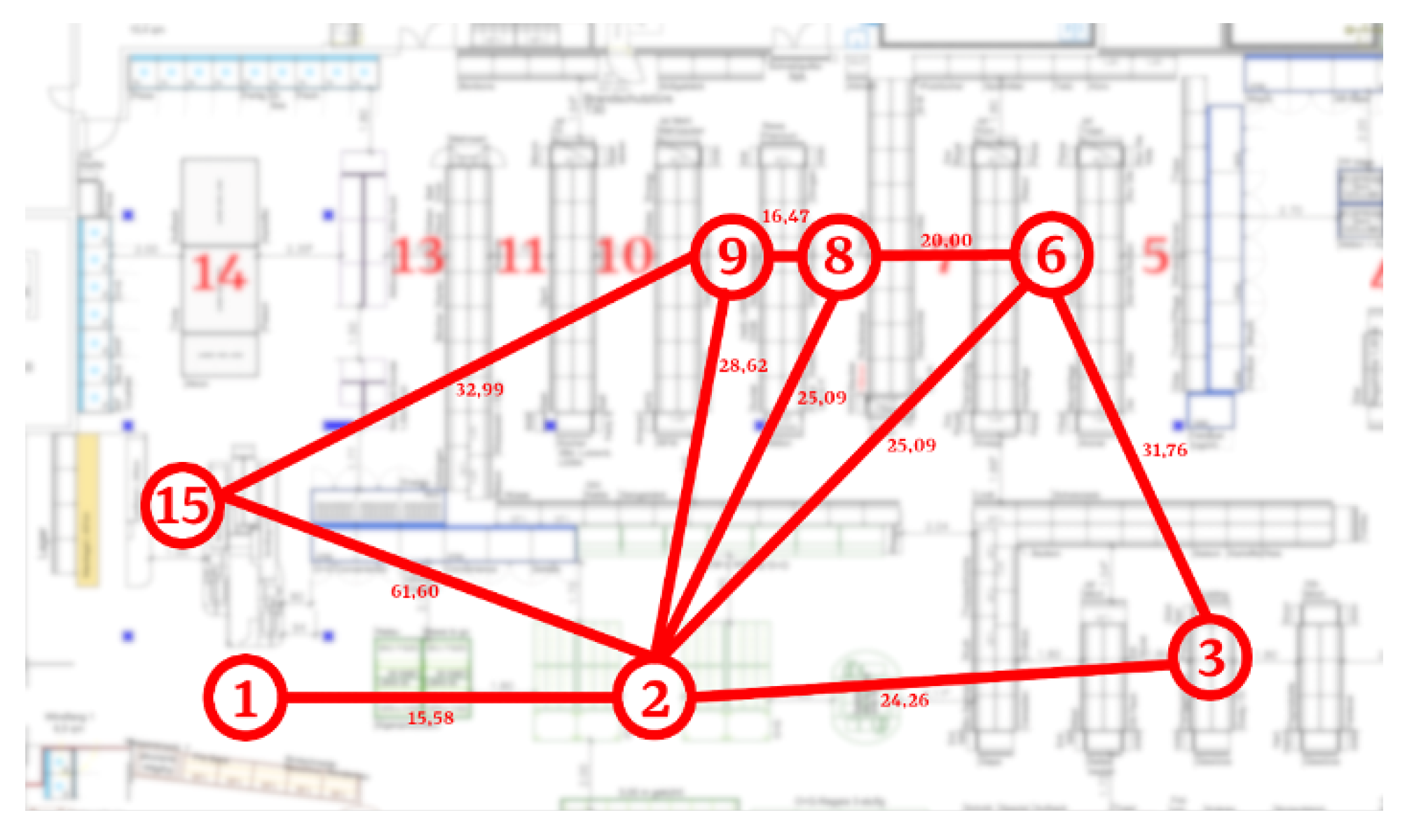
The research is based on data made available by a German retailer with the layout of one of their stores and real BOPS orders placed online to be picked up at the store. Following the idea of [17,18], the layout of the store was divided into 15 zones (Figure 1) according to the locations and product categories. Zone 1 contained the entrance and zone 15 contained the exit. Each product is located in a certain zone. By assuming each product in the given zone has an equal probability of being picked, we are able to define the center of zones and calculate the approximated distances $d_{ij}$ between zone i and zone j ($i\ne j|i,j\in \{1,2,\dots ,15\}$). With a walking speed estimated at 0.85 m/s, the approximate travel time between different zones is shown in

Table 1. Approximate travel time (s) between different zones in the reference store.

${\mathit{t}}_{\mathit{i}\mathit{j}}$	1	2	3	4	5	6	7	8	9	10	11	12	13	14	15
1		15.58	39.84	49.84	44.20	40.67	37.14	40.67	44.20	47.73	51.26	70.33	65.96	74.83	77.18
2	15.58		24.26	34.26	28.62	25.09	21.56	25.09	28.62	32.15	35.68	54.75	50.39	59.25	61.60
3	39.84	24.26		24.06	29.07	31.76	28.24	31.76	35.29	38.82	42.35	61.42	57.06	65.92	68.28
4	49.84	34.26	24.06		21.91	25.44	28.97	32.50	36.02	39.55	43.08	62.15	57.79	66.65	69.01
5	44.20	28.62	29.07	21.91		16.47	20.00	23.53	27.06	30.59	34.12	53.18	48.82	57.69	60.04
6	40.67	25.09	31.76	25.44	16.47		16.47	20.00	23.53	27.06	30.59	49.66	45.29	54.16	56.51
7	37.14	21.56	28.24	28.97	20.00	16.47		16.47	20.00	23.53	27.06	46.13	41.76	50.63	52.98
8	40.67	25.09	31.76	32.50	23.53	20.00	16.47		16.47	20.00	23.53	29.66	25.29	34.16	36.52
9	44.20	28.62	35.29	36.02	27.06	23.53	20.00	16.47		16.47	20.00	26.13	21.76	30.64	32.99
10	47.73	32.15	38.82	39.55	30.59	27.06	23.53	20.00	16.47		16.47	22.60	18.24	27.11	29.46
11	51.26	35.68	42.35	43.08	34.12	30.59	27.06	23.53	20.00	16.47		19.07	14.71	23.57	25.92
12	70.33	54.75	61.42	62.15	53.18	49.66	46.13	29.66	26.13	22.60	19.07		13.77	22.64	29.69
13	65.96	50.39	57.06	57.79	48.82	45.29	41.76	25.29	21.76	18.24	14.71	13.77		17.59	14.26
14	74.83	59.25	65.92	66.65	57.69	54.16	50.63	34.16	30.64	27.11	23.57	22.64	17.59		7.20
15	77.18	61.60	68.28	69.01	60.04	56.51	52.98	36.52	32.99	29.46	25.92	29.69	14.26	7.20

.

A BOPS order is a list of products to be picked by an employee of the store. To complete our simulation analysis in this work, each product has the attributes of volume, mass, density and type of packaging on top of the zone containing it.

As stated in Section 1, for retailers such as the one under investigation, there is currently no optimization being developed relative to the in-store picking process of BOPS orders. A list of articles is usually presented alphabetically or randomly to the person in charge. After a preliminary review of the list, an experienced employee normally uses the store topology to self-organize a time- and distance-saving path through the store based on their knowledge of the store. In practice, however, pickup of online orders is frequently assigned to part-time workers with marginal experience. In such a case, a simple optimization aiming at minimizing the travel distance to fulfill the orders can be proposed. Extended modeling with impacts of the employees’ characteristics on the optimization approach is expected in a future work.

In the following subsections, we introduce three shortest path-like analyses that focus on different aspects to optimize the picking process.

3.2. The Open Traveling Salesman Problem

An Open Traveling Salesman Problem (TSP) is an NP-hard problem in the field of combinatorial optimization that asks the following question: ‘Given a list of customers to whom some products have to be transported, what is the shortest route that connects a start depot (at which products are loaded) and an end depot (where the vehicle is parked after the tour) while visiting all customers?’

The problem can therefore be represented by a weighted directed graph $G=(V,E)$, where V is the set of customers/depots that needs to be visited, and $E=\left\{\right(i,j\left)\right|i,j\in V\}$ is the set of edges connecting all the vertices pairs. To each edge $e\in E$ a cost $c_{ij}$ is associated, which can be the distance or the time required to travel from customer/depot i to customer/depot j. The objective is to find the set S of edges that connects the start and end points in such a way that each vertex in V is considered one and only one time, all the edges are adjacent, and the sum of the costs ${\sum }_{(i,j)\in S}{t}_{ij}$ is minimized.

The TSP can be formulated and solved easily since it has been well studied by many approaches [23,24,25].

As in-store logistics is one of the main cost drivers, it has been proven that sequencing the orders by the TSP solution can effectively improve the picking time performance [18]. However, as mentioned earlier, the lack of consideration in item placement inside bags can lead to potential product damage, thus, an extra time cost is expected for rearrangements. Therefore, a constraints based on product attributes should be considered [19] with respect to the shortest route analysis. The problem is then solved as a Sequential Ordering Problem in the following section.

3.3. The Sequential Ordering Problem

A Sequential Ordering Problem (SOP) is again an NP-hard problem in the field of combinatorial optimization that asks a question similar to the open TSP: ‘Given a start depot, a list of customers, and an end depot, with the distances between each pair of depot-customer or customer-customer and a set of precedence constraints between customers, which is the optimal shortest route that connects the start and end depot while visiting all the customers and satisfying the precedence constraints?’

The SOP formulations and solvers can be found in [20,26,27,28].

In this problem, we sorted the products from the most resistant to the most fragile. Therefore, we defined the precedence on the products not zones. A priority score was assigned to each product based on chosen attributes combined through a weighted sum model. We applied the scoring model proposed in a previous work [19], in which the scores(SC) for mass, volume, and density were defined by ad hoc piecewise functions simulated by the impacts of the attributes based on their value. The scores for the packaging type (packSC) were assigned based on estimated sturdiness. The weights of the attributes were manually adjusted based on real-world simulations. In this work, the weights are given as follows:

$$SC=massSC·0.15+volumeSC·0.15+densitySC·0.30+packSC·0.40$$

By turning the scores of the articles into the precedence constraints, the in-store picking problem could be solved as the SOP defined. Note that the scores in this work were defined for the retailer we studied, which considered basic requirements. It can also be adjusted or extended to fit with specific needs such as the temperature, potential water vapor effects on paper packages, and the smell of certain fresh foods.

3.4. The Relaxed SOP

In reality, if we strictly followed all the precedence constraints in the SOP, a lot of back and forward movements would be expected, which would lead to significantly longer times to complete the picking operation. This inefficiency is contrary to the original intention of the benefits of solving the problem as a SOP. Therefore, in this section, we propose a Relaxed SOP model to create a tradeoff between priorities and total picking time.

By assuming that products with similar priority scores have similar characteristics in terms of fragility/sturdiness, a tradeoff between damage prevention and time required for the operation can be achieved by defining a limited number of precedence classes, each one containing products with similar characteristics that can be considered as equivalent in terms of damage resistance. In such a way, each product is assigned to one of the subgroups depending on its priority score. Precedence among products in the same group is then relaxed. The number of classes can be adjusted depending on specific needs. In this work, we divided the products into four precedence classes.

4. The Packing Problem

In Section 3, we introduced different in-store routing methodologies that can optimize the picking process. With the implementation of a ‘scan-as-you-pick device’ that is gradually becoming popular in stores, the employees performing the picking operation are able to scan and pack the products during the picking process without the need of a cashier later on to produce the bill. In such a context, employees could, however, have difficulty distributing evenly and safely all the products into the shopping bags, in order to avoid too heavy/full or light/empty imbalance issues.

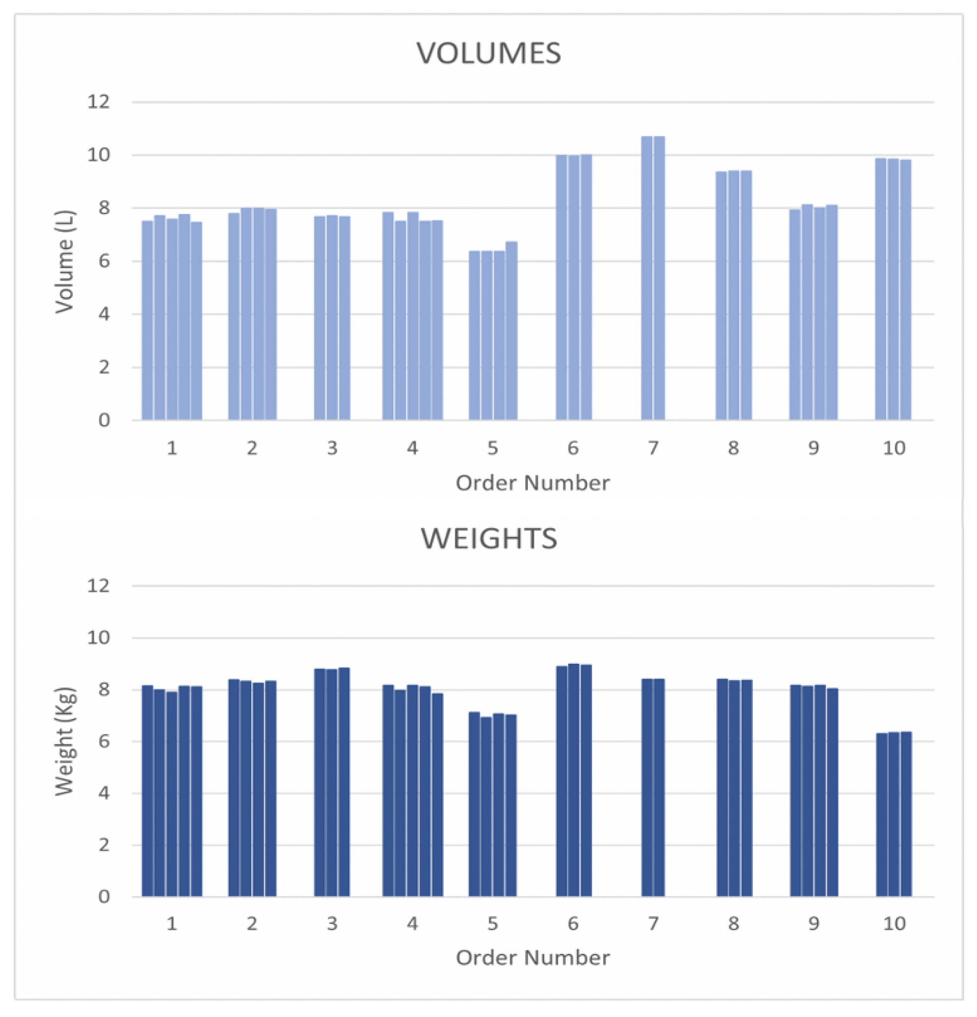
To solve this problem and make the packing operation more efficient, a two-step optimization is developed, as described in [29], that first calculates the minimum number of bags needed for a given shopping list and balances the content of the bags by minimizing the differences of weight and volume of the products contained in each pair of bags. The first step is to determine the minimum number of bags required $b_{min}$ for a given shopping list. The following formulation is based on a classic Bin Packing problem [21]. We define $P=\{1,2...,m\}$ as the set of products and $B=\{1,2...,n\}$ as the set of available shopping bags. The volume and weight of each product $i\in P$ are represented as $v_i$ and $w_i$, respectively. The content of each shopping bag cannot exceed a maximum volume $V_{max}$ and a maximum weight $W_{max}$. Two binary variables are also defined: $x_{ij}$ takes the value 1 if product i is in packed bag j, 0 otherwise, and $y_j=1$ if bag j is used, 0 otherwise. The problem can be then written in the following way:

$$\begin{array}{cc}\hfill b_{min}=min& \sum _{j\in B}{y}_j\hfill \end{array}$$

(1)

$$\begin{array}{ccc}\hfill s.t& \sum _{i\in P}{w}_i{x}_{ij}\le W_{max}{y}_j\hfill & \hfill \hspace{1em}\hspace{1em}j\in B\end{array}$$

(2)

$$\begin{array}{ccc}\hfill & \sum _{i\in P}{v}_i{x}_{ij}\le V_{max}{y}_j\hfill & \hfill \hspace{1em}\hspace{1em}j\in B\end{array}$$

(3)

$$\begin{array}{ccc}\hfill & \sum _{j\in B}{x}_{ij}=1\hfill & \hfill \hspace{1em}\hspace{1em}i\in P\end{array}$$

(4)

$$\begin{array}{ccc}\hfill & x_{ij}\in \{0,1\}\hfill & \hfill \hspace{1em}\hspace{1em}i\in P,j\in B\end{array}$$

(5)

$$\begin{array}{ccc}\hfill & y_j\in \{0,1\}\hfill & \hfill \hspace{1em}\hspace{1em}j\in B\end{array}$$

(6)

The constraints (2) and (3) restrict the articles in each bag from exceeding the maximum weight and volume. Constraint (4) enforces each article to be in one and only one bag.

When there is more than one bag required for the shopping list, the second optimization step is to balance the contents of the bags as evenly as possible. This is realized by solving a Min-Max problem [30]. We define $B_m=\{1,...,b_{min}\}$ as the set of bags to be used, z as the minmax variable. $d_w^{+}$,$d_w^{-}$,$d_v^{+}$ and $d_v^{-}$ are technical variables required to minimize the difference between the volume and weight of each pair of bags. The problem can be written as follows:

$$\begin{array}{cc}\hfill min& z\hfill \\ \hfill s.t& \left(2\right)-\left(6\right)\hfill \end{array}$$

(7)

$$\begin{array}{ccc}\hfill & \sum _{i\in P}{w}_i{x}_{ij}-\sum _{i\in P}{w}_i{x}_{ik}-d_w^{+}+d_w^{-}=0\hfill & \hfill \hspace{1em}\hspace{1em}j,k\in B_m,j<k\end{array}$$

(8)

$$\begin{array}{ccc}\hfill & \sum _{i\in P}{v}_i{x}_{ij}-\sum _{i\in P}{v}_i{x}_{ik}-d_v^{+}+d_v^{-}=0\hfill & \hfill \hspace{1em}\hspace{1em}j,k\in B_m,j<k\end{array}$$

(9)

$$\begin{array}{cc}\hfill & z\ge d_w^{+}+d_w^{-}\hfill \end{array}$$

(10)

$$\begin{array}{cc}\hfill & z\ge d_v^{+}+d_v^{-}\hfill \end{array}$$

(11)

$$\begin{array}{ccc}\hfill & d_w^{+},d_w^{-},d_v^{+},d_v^{-}\ge 0\hfill & \hfill \end{array}$$

(12)

With constraint (8) and (9), each shopping bag contains products that sum up to a similar volume and weight. The minmax constraints for the distance variables are shown in (10) and (11). The distance variables $d_w^{+}$,$d_w^{-}$,$d_v^{+}$ and $d_v^{-}$ are nonnegative.

In practice, different types of bags may be required for different products. In such a case, the products should first be classified according to the type of bag required, then the algorithm can be applied to each subgroup. As minimizing the number of bags is an environmental friendly intention, customers can also choose to use paper bags, reusable plastic boxes, or their own bags for the same purpose. Correspondingly, the classification of the products based on the bags can be customized. The model itself is adaptable to these changes.

5. Combined Picking and Packing

By applying the packing process with the two-step optimization in Section 4, it is easy to combine with the picking strategies in Section 3 that indicate the proper route to pick the articles in a certain order. The hybrid strategies allow the employee to collect each item, scan it and place it in the final shopping bag all at the same time. The shopping bags are then ready to go at the end of a picking process.

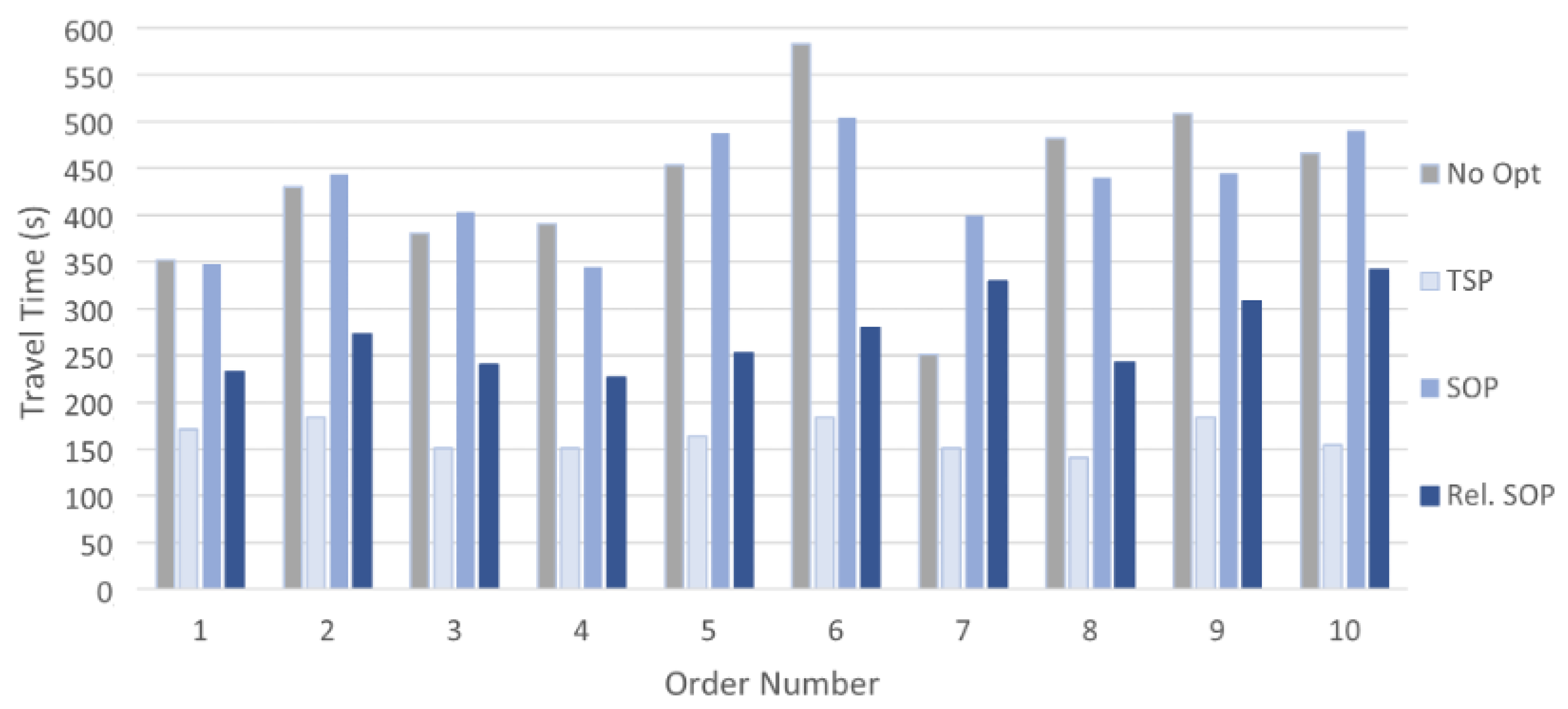
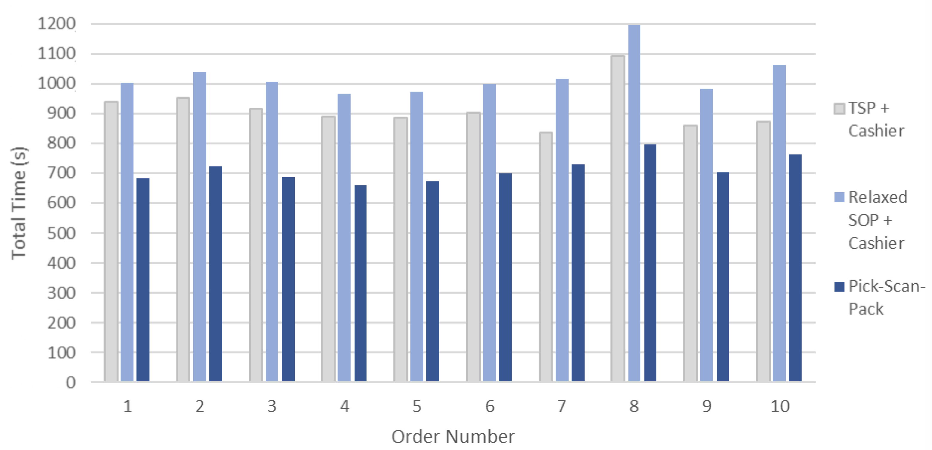
For a comprehensive understanding of optimization strategies in both the picking and packing process, we consider the following scenarios:

• TSP solution in which products are scanned and packed at the cashier (this will be referred to as TSP + cashier);
• SOP solution in which products are scanned and packed at the cashier (this will be referred to as SOP + cashier);
• SOP solution in which products are scanned and packed during the picking operation by using a scan-as-you-pick device (this will be referred to as pick-scan-pack model for SOP);
• Relaxed SOP solution in which products are scanned and packed at the cashier (this will be referred to as Relaxed SOP + cashier);
• Relaxed SOP solution in which products are scanned and packed during the picking operation by using a scan-as-you-pick device (this will be referred to as pick-scan-pack model for Relaxed SOP).

We do not consider the scenario of TSP with scan-as-you-pick device because of potential damage to the products.

6. Experimental Simulations

In this section, we present the results of an experimental simulation carried out on a real store located in Germany (see Section 3.1). We considered 10 representative real BOPS orders that consisted of 48 items on average with a standard deviation of 5. The different methods introduced in Section 3 and Section 4 are compared. All necessary calculations were performed on Microsoft Excel 2019.

6.1. Picking

We started with the picking strategies presented in Section 3. The following scenarios were considered: no optimization, the TSP solution, the SOP solution, and the Relaxed SOP solution.

6.1.1. No Optimization

First, we present a scenario that did not implement any optimization to show the performance of a baseline: a randomly ordered list with no indications on product locations is assigned to an employee with a low level of knowledge of the store layout. In this scenario, the employee picks the items one by one following the order of appearance on the shopping list. The simulation of travel times for the 10 orders considered are reported in

Table 2. Simulation of travel times for 10 BOPS orders when no optimization is implemented.

Order 1		Order 2		Order 3		Order 4		Order 5
$t_{ij}$	Zone	$t_{ij}$	Zone	$t_{ij}$	Zone	$t_{ij}$	Zone	$t_{ij}$	Zone
/	1	/	1	/	1	/	1	/	1
51.26	11	51.26	11	51.26	11	51.26	11	51.26	11
25.92	12	25.92	12	22.04	12	25.92	12	25.92	12
29.46	10	29.46	10	29.46	10	29.46	10	29.46	10
29.46	12	16.47	11	16.47	11	29.46	12	16.47	11
29.46	10	16.47	10	16.47	10	29.46	10	16.47	10
29.46	12	16.47	11	29.46	12	29.46	12	16.47	11
29.46	10	16.47	10	29.46	10	29.46	10	25.92	12
27.06	6	29.46	12	29.46	12	29.46	12	29.46	10
31.76	3	29.46	10	29.46	10	29.46	10	29.46	12
68.28	15	29.46	12	16.47	11	38.82	3	29.46	10
		29.46	10	42.35	3	68.28	15	16.47	11
		27.06	6	68.28	15			42.35	3
		31.76	3					28.24	7
		28.24	7					28.24	3
		52.98	15					68.28	15
351.58 s		430.40 s		380.63 s		390.50 s		453.92 s
Order 6		Order 7		Order 8		Order 9		Order 10
$t_{ij}$	Zone	$t_{ij}$	Zone	$t_{ij}$	Zone	$t_{ij}$	Zone	$t_{ij}$	Zone
/	1	/	1	/	1	/	1	/	1
51.26	11	51.26	11	15.58	2	51.26	11	44.20	9
25.92	12	16.47	10	28.62	9	22.04	12	16.47	8
25.92	11	29.46	12	16.47	8	29.46	10	25.09	2
25.92	12	25.92	11	16.47	9	16.47	11	28.62	9
25.92	11	35.68	2	35.29	3	25.92	12	20.00	11
16.47	10	24.26	3	35.29	9	29.46	10	42.35	3
16.47	11	68.28	15	16.47	8	29.46	12	42.35	11
16.47	10			31.76	3	29.46	10	23.53	8
29.46	12			35.29	9	29.46	12	31.76	3
29.46	10			35.29	3	29.46	10	31.76	8
29.46	12			31.76	8	16.47	9	31.76	3
29.46	10			31.76	3	23.53	6	35.29	9
27.06	6			31.76	8	23.53	9	16.47	8
31.76	3			31.76	3	35.29	3	20.00	6
35.29	9			31.76	6	39.84	1	56.51	15
35.29	3			56.51	15	77.18	15
583.42 s		251.33 s		481.89 s		508.29 s		466.19 s

. The shopping list of each order (columns) is presented by locations (zones) of the products and travel times ($t_{ij})$ between different zones when the products are being picked.

6.1.2. The TSP Solution

As mentioned in Section 3.2, the Traveling Salesman Problem can be adapted to the problem we study by treating the shopping cart as the vehicle and the zones to visit as the customers: zone 1 represents the “start depot” as it contains the entry while zone 15 represents the “end depot” since the shopping bags are stored here when waiting to be picked up. The set V of vertices that makes up the graph G is a subset of the zones set that contains zone 1, zone 15, and the zones from which at least one product needs to be picked up. Since with this solution each zone must be visited only once, all the products in the same zone should be grouped together and collected when arriving at each zone. For example, order 8 contains products from the following zones: 1, 2, 9, 8, 3, 6, and 15 (1 and 15 are included by default as they are the start and end points). The zones are highlighted on the layout in Figure 2. The edges are constructed according to the vertices contained in V, and the respective cost associated with each edge can be retrieved from the Origin-Destination travel time matrix in Table 1 in Section 3.1. This operation is represented partly in Figure 2 for better understanding. The shopping list is rearranged according to the TSP optimal solution that gives the lowest travel time between the zones. The travel times for the BOPS orders when the TSP optimization is implemented are shown in

Table 3. Simulation of travel times for 10 BOPS orders when the TSP optimization is implemented.

Order 1		Order 2		Order 3		Order 4		Order 5
$t_{ij}$	Zone	$t_{ij}$	Zone	$t_{ij}$	Zone	$t_{ij}$	Zone	$t_{ij}$	Zone
/	1	/	1	/	1	/	1	/	1
39.84	3	39.84	3	39.84	3	39.84	3	39.84	3
31.76	6	31.76	6	38.82	10	38.82	10	28.24	7
27.06	10	16.47	7	16.47	11	16.47	11	23.53	10
16.47	11	23.53	10	25.92	12	25.92	12	16.47	11
25.92	12	16.47	11	29.69	15	29.69	15	25.92	12
29.69	15	25.92	12					29.69	15
		29.69	15
170.75 s		183.69 s		150.75 s		150.75 s		163.69 s
Order 6		Order 7		Order 8		Order 9		Order 10
$t_{ij}$	Zone	$t_{ij}$	Zone	$t_{ij}$	Zone	$t_{ij}$	Zone	$t_{ij}$	Zone
/	1	/	1	/	1	/	1	/	1
39.84	3	15.58	2	15.58	2	39.84	3	15.58	2
31.76	6	24.26	3	24.26	3	31.76	6	24.26	3
23.53	9	38.82	10	31.76	6	23.53	9	31.76	6
16.47	10	16.47	11	20.00	8	16.47	10	20.00	8
16.47	11	25.92	12	16.47	9	16.47	11	16.47	9
25.92	12	29.69	15	32.99	15	25.92	12	20.00	11
29.69	15					29.69	15	25.92	15
183.69 s		150.75 s		141.06 s		183.69 s		154.00 s

. It is a coincidence that all lists are sorted in ascending order, due to how the zones are numbered.

6.1.3. The SOP Solution

As mentioned in Section 3.3, the Sequential Ordering Problem was adapted to the problem we study in this section. Different from the TSP solution, a zone can be visited on multiple occasions to pick up products with different priorities, thus the set V of vertices is associated with the products, and each vertex/product is characterized by the two labels (zone and priority score). The edges are constructed according to the vertices contained in V, and the cost associated with each edge can be retrieved from the Origin-Destination travel time matrix in Table 1. To find the optimal SOP solution, we first simplify the graph by sorting the vertices in ascending order in terms of priority score. Simulation of travel times for the BOPS orders with the optimal SOP solution are reported in

Table 4. Simulation of travel times for 10 BOPS orders when the SOP optimization is implemented.

Order 1			Order 2			Order 3			Order 4			Order 5
$t_{ij}$	Zone	$SC$	$t_{ij}$	Zone	$SC$	$t_{ij}$	Zone	$SC$	$t_{ij}$	Zone	$SC$	$t_{ij}$	Zone	$SC$
/	1	/	/	1	/	/	1	/	/	1	/	/	1	/
47.73	10	14.10	51.26	11	14.70	51.26	11	14.70	47.73	10	14.10–14.70	51.26	11	14.70
29.46	12	14.10	25.92	12	14.10	16.47	10	14.10	16.47	11	13.50	25.92	12	14.10
16.47	11	13.50	25.92	11	13.50	16.47	11	13.50	25.92	12	12.90	25.92	11	13.50
16.47	10	12.90–13.50	25.92	12	12.90	25.92	12	12.90	29.46	10	11.85–12.90	16.47	10	11.85–12.90
27.06	6	11.25	29.46	10	9.65–12.90	25.92	11	12.15	29.46	12	11.30–11.85	29.46	12	11.25–11.85
31.76	3	11.25	29.46	12	9.65	25.92	12	11.85	29.46	10	9.65–11.25	29.46	10	10.65-11.25
61.42	12	11.25	22.04	11	9.05	29.46	10	11.85–11.25	29.46	12	9.65	29.46	12	9.65
29.46	10	9.90–11.25	16.47	10	8.75–9.05	29.46	12	11.25–9.65	29.46	10	8.75–9.20	29.46	10	9.05–9.65
29.46	12	9.65	38.82	3	8.10–8.50	29.46	10	9.65–9.05	38.82	3	8.50	16.47	11	9.05
29.46	10	6.45–9.65	28.24	7	6.65	16.47	11	9.05	38.82	10	5.85–8.10	16.47	10	8.75
29.46	15		23.53	10	5.85–6.45	16.47	10	8.75	29.46	15		23.53	7	8.50
			27.06	6	4.50–4.95	38.82	3	8.50				28.24	3	8.50
			31.76	3	3.35	38.82	10	5.85				38.82	10	5.85
			68.28	15		16.47	11	3.95–3.65				16.47	11	3.80
						25.92	15					42.35	3	3.35
												68.28	15
348.21 s			444.14 s			403.33 s			344.52 s			488.04 s
Order 6			Order 7			Order 8			Order 9			Order 10
$t_{ij}$	Zone	$SC$	$t_{ij}$	Zone	$SC$	$t_{ij}$	Zone	$SC$	$t_{ij}$	Zone	$SC$	$t_{ij}$	Zone	$SC$
/	1	/	/	1	/	/	1	/	/	1	/	/	1	/
70.30	12	14.10	47.73	10	13.50	39.84	3	12.90	47.73	10	14.10–14.70	44.20	9	13.25
25.92	11	13.50	16.47	11	13.50	31.76	6	11.85	16.47	11	13.50	23.53	6	12.90
25.92	12	11.25–12.90	25.92	12	11.25	31.76	3	11.25–11.85	16.47	10	12.90–13.50	30.58	11	11.85–12.90
29.46	10	10.95–11.25	61.42	3	9.10	24.26	2	10.70	29.46	12	11.25–12.90	42.35	3	10.65–11.25
29.46	12	9.65	38.82	10	8.75	24.26	3	9.35–10.65	49.65	6	11.25	31.76	8	10.40
25.92	11	9.05	38.82	3	6.00	35.29	9	9.35	31.76	3	11.25	31.76	3	10.35
16.47	10	8.75–9.05	42.35	11	5.40	16.47	8	9.20	39.84	1	11.25	24.26	2	9.65
38.82	3	8.50	42.35	3	4.95	16.47	9	7.60–8.75	47.73	10	9.65–10.95	28.62	9	9.05
35.29	9	8.50	24.26	2	3.95	16.47	8	7.45–7.60	29.46	12	9.05–9.65	16.47	8	7.75
16.47	10	6.45	35.68	11	3.80	16.47	9	7.30	25.92	11	9.05	16.47	9	7.30–7.45
27.06	6	6.45	25.92	15		35.29	3	7.15	42.35	3	8.10	16.47	8	6.00–6.60
31.76	3	5.25–6.00				35.29	9	7.15	35.29	9	2.90–5.10	20.00	6	5.85–6.00
31.76	6	4.95				16.47	8	6.30–6.60	32.99	15		31.76	3	5.35
31.76	3	3.35–4.95				31.76	3	3.35–5.35				31.76	8	5.10
68.28	15					68.28	15					31.76	3	2.90–3.95
												68.28	15
504.68 s			399.76 s			440.16 s			445.13 s			490.05 s

.

6.1.4. The Relaxed SOP Solution

In Section 3.3, we also introduced a Relaxed SOP, in which the priority scores are replaced by the precedence classes ($PC$). In such a case, the set V of vertices is composed by (zone and precedence class) pairs. Simulation of travel times for the BOPS orders with the optimal Relaxed SOP solution are reported in

Table 5. Simulation of travel times for 10 BOPS orders when the Relaxed SOP optimization is implemented.

Order 1			Order 2			Order 3			Order 4			Order 5
$t_{ij}$	Zone	$PC$	$t_{ij}$	Zone	$PC$	$t_{ij}$	Zone	$PC$	$t_{ij}$	Zone	$PC$	$t_{ij}$	Zone	$PC$
/	1	/	/	1	/	/	1	/	/	1	/	/	1	/
47.73	10	4	47.73	10	4	47.73	10	4	47.73	10	4	47.73	10	4
16.47	11	4	16.47	11	4	16.47	11	4	16.47	11	4	16.47	11	4
25.92	12	4-3	25.92	12	4-3	25.92	12	4-3	25.92	12	4-3	25.92	12	4-3
42.21	6	3	25.92	11	3	25.92	11	3	29.46	10	3-2	25.92	11	3
31.76	3	3	16.47	10	3-2	16.47	10	3-2	38.82	3	2	16.47	10	3-2
38.82	10	3-2	23.53	7	2	38.82	3	2	68.28	15		23.53	7	2
29.46	15		28.24	3	2-1	42.35	11	1				28.24	3	2-1
			31.76	6	1	25.92	15					42.35	11	1
			56.51	15								25.92	15
232.38 s			272.56 s			239.62 s			226.68 s			252.56 s
Order 6			Order 7			Order 8			Order 9			Order 10
$t_{ij}$	Zone	$PC$	$t_{ij}$	Zone	$PC$	$t_{ij}$	Zone	$PC$	$t_{ij}$	Zone	$PC$	$t_{ij}$	Zone	$PC$
/	1	/	/	1	/	/	1	/	/	1	/	/	1	/
51.26	11	4	47.73	10	4	39.84	3	4-3	47.73	10	4	40.67	6	4
25.92	12	4-3	16.47	11	4	24.26	2	3	16.47	11	4	23.53	9	4
25.92	11	3	25.92	12	3	25.09	6	3	25.92	12	4-3	20.00	11	4-3
16.47	10	3-2	29.46	10	3	20.00	8	3	25.92	11	3	20.00	9	3
16.47	9	2	38.82	3	3-2	16.47	9	3-2	16.47	10	3	16.47	8	3
23.53	6	2	42.35	11	2-1	16.47	8	2	47.73	1	3	25.09	2	3
31.76	3	2-1	42.35	3	1	31.76	3	2-1	39.84	3	3-2	24.26	3	3-2
31.76	6	1	24.26	2	1	68.28	15		31.76	6	2	31.76	6	2
56.51	15		61.60	15					23.53	9	2-1	20.00	8	2
									32.99	15		16.47	9	2
												35.29	3	1
												68.28	15
279.62 s			328.98 s			242.17 s			308.37 s			341.83 s

.

6.1.5. Time Performance Analysis

The results of the simulations in terms of the picking process are summarized in Figure 3 and

Table 6. Comparison between simulated travel times with different routing strategies implemented for 10 BOPS orders.

	Order 1	Order 2	Order 3	Order 4	Order 5
No Opt	351.58	430.40	380.63	390.50	453.92
TSP	170.75	183.69	150.75	150.75	163.69
SOP	348.21	444.14	403.33	344.52	488.04
Rel. SOP	232.38	272.56	239.62	226.68	252.56
	Order 6	Order 7	Order 8	Order 9	Order 10
No Opt	583.42	251.33	481.89	508.29	466.19
TSP	183.69	150.75	141.06	183.69	154.00
SOP	504.68	399.76	440.16	445.13	490.05
Rel. SOP	279.62	328.98	242.17	308.37	341.83

.

In Table 6, we can observe clearly that the TSP optimization has the best performance in terms of travel time, so our main interest is in estimating the extra time required by optimizing with the SOP solutions, and whether this extra time is worth being invested to have a better sequencing of the articles. When considering the optimal TSP solution, the picking operation takes 163.28 s on average, the optimal SOP solution takes 430.80 s, meanwhile the Relaxed SOP takes 272.48 s on average. Note that the SOP-based strategies preserve the articles’ integrity by avoiding damage, although this factor is not captured by the times represented here. Considering the fact that in-store logistics operations are a major cost driver and human resources are required for all in-store activities [31], the Relaxed SOP offers a good tradeoff by sacrificing a bit more time than TSP while preventing damage to the products. The more constraining SOP is less competitive in this sense since it takes too long. Furthermore, the high amount of back and forward movements by store employees may interfere with regular in-shop customers and lower their satisfaction levels. Meanwhile, the time difference between the TSP and Relaxed SOP can possibly be regained while considering packaging time as well. Packing the products while they are being picked may save time, but the more constraining SOP cannot accomplish this due to the significant difference.

6.2. Packing

We then move to the packing process described in Section 4. We reproduced the calculation results in [29] to calculate the number of shopping bags required and to distribute all the articles homogeneously among the bags: the maximum difference in terms of volume and weight between all the shopping bags for a certain shopping list is 0.36 L 0.32 kg. The simulation results of the model are reported in Figure 4. For each of the 10 orders, we show the estimated number of bags and the total volume and weight of the articles in each shopping bag.

In Figure 4, we can observe that the products are divided evenly in each shopping bag in terms of volumes and weights (each column in the chart represents a bag). In such a way, the shopping list given to the employees is fully optimized, and no rearrangement is required after the picking process.

6.3. Picking and Packing

With the help of the two-step optimization in the previous section, it is possible to estimate the total time required to complete a SOP-based picking and packing operation in a reliable way. With analogous considerations, it is also possible to estimate the time spent at the cashier for the TSP picking and packing operation. Therefore, in this section, we compare the total time cost considering both the picking and packing process as described in Section 5.

In this simulation, we no longer consider the SOP solution for the reasons given in Section 6.1. Therefore, we consider only three out of five scenarios described in Section 5:

• TSP + cashier;
• Relaxed SOP + cashier; and
• pick-scan-pack model for Relaxed SOP.

In all scenarios, 2 s per bag is necessary for preparation. The travel times are derived directly from Section 6.1 for the TSP and Relaxed SOP. Once a zone is reached, each item has an equal probability of being picked, the time to locate and pick the item is estimated as 7 s if it is directly placed in the shopping cart without scanning it or 9 s if the pick-scan-pack model is applied. When the pick-scan-pack model is not implemented, two employees will be occupied at the cashier: the picker and the cashier. The necessary time to complete the loading, scanning, and packing procedure is estimated as 5 s per product for the picker (0.5 to place the items on the conveyor belt, 2.5 for the product to get from the loading point to the scanning point [32], 0.5 to scan the product, and finally 1.5 to place the item into a bag) and 3.5 s per product for the cashier (0.5 for the items to be placed on the conveyor belt, 2.5 for the product to get from the loading point to the scanning point [32], and 0.5 to scan the product). The simulation results are reported in Figure 5.

From the figure it can be observed that the pick-scan-pack model for Relaxed SOP performs the best. The time difference ranges between 107.78 s and 295.39 s with an average of 202.81 s when compared to the TSP+cashier scenario, and between 279.50 s and 396.50 s with an average of 312.00 s when compared to the Relaxed SOP + cashier scenario. This means that the pick-scan-pack alternative reduces the total time needed by 22.18% and 30.48%. It shows a remarkable improvement that underlines even further the efficiency of the Relaxed SOP optimization when paired with the right instruments (scan-as-you-pick devices) and models (the packing model).

For the reasons above, the Relaxed SOP is considered the best and most applicable optimization approach with the following advantages:

• Prevents product damaging without excessively increasing picking time.
• Allows the integration of picking and packing operations.

7. Conclusions

This research on optimization strategies for Buy-Online-Pick-up-in-Store order fulfillment aspired to improve omnichannel in-store logistics operations for brick-and-mortar grocery retails. The aim of the present study was, in particular, to provide process optimization tools for retailing shops. Different optimization approaches were discussed for the in-store order picking and packing problem. With experimental simulations carried out on real orders, we demonstrated that the optimization on routing performs better in terms of damage prevention and does not increase the travel time required. Moreover, it gives the possibility to pick safely, scan, and pack the products simultaneously. With further optimization that balances the distribution of products in different shopping bags coupled with the use of scan-as-you-pick devices, the performance of the overall optimization strategy is excellent.

All optimizations discussed in this work are practical and easily applicable in most Buy-Online-Pick-up-in-Store systems. Further extensions of the work can also move from the deterministic to stochastic settings by considering the modeling of the pickers’ behavior and the presence of regular walk-in customers.

References

1. Hübner, A.; Wollenburg, J.; Holzapfel, A. Retail logistics in the transition from multi-channel to omni-channel. Int. J. Phys. Distrib. Logist. Manag. 2016, 46, 562–583. [Google Scholar] [CrossRef]
2. Bell, D.R.; Gallino, S.; Moreno, A. How to win in an omni-channel world. MIT Sloan Manag. Rev. 2014, 56, 45–55. [Google Scholar]
3. Rigby, D. The future of shopping. Harv. Bus. Rev. 2011, 89, 65–76. [Google Scholar]
4. Wollenburg, J.; Hübner, A.; Kuhn, H.; Trautrims, A. From bricks-and-mortar to bricks-and-clicks: Logistics networks in omni-channel grocery retailing. Int. J. Phys. Distrib. Logist. Manag. 2018, 48, 415–438. [Google Scholar] [CrossRef]
5. Jin, M.; Li, G.; Cheng, T.C.E. Buy online and pick up in-store: Design of the service area. Eur. J. Oper. Res. 2018, 268, 613–623. [Google Scholar] [CrossRef]
6. Kong, R.; Luo, L.; Chen, L.; Keblis, M.F. The effects of BOPS implementation under different pricing strategies in omnichannel retailing. Transp. Res. Part E Logist. Transp. Rev. 2020, 141, 102014. [Google Scholar] [CrossRef]
7. Fan, C.; Liu, Y.; Yang, X.; Chen, X.; Hu, J. Online and offline cooperation under buy-online, pick-up-in-store: Pricing and inventory decisions. J. Ind. Manag. Optim. 2019, 15, 1455–1472. [Google Scholar] [CrossRef]
8. Saha, K.; Bhattacharya, S. ‘Buy online and pick up in-store’: Implications for the store inventory. Eur. J. Oper. Res. 2020, 294, 906–921. [Google Scholar] [CrossRef]
9. Lin, X.; Zhou, Y.; Hou, R. Impact of a “Buy-online-and-pickup-in-store” Channel on Price and Quality Decisions in a Supply Chain. Eur. J. Oper. Res. 2021, 294, 922–935. [Google Scholar] [CrossRef]
10. Lu, J.; Yang, Y.; Han, S.; Tsao, Y.; Xin, Y. Coordinated inventory policies for meeting demands from both store and online BOPS channels. Comput. Ind. Eng. 2020, 145, 106542. [Google Scholar] [CrossRef]
11. Shi, X.; Dong, C.; Cheng, T.C.E. Does the buy-online-and-pick-up-in-store strategy with pre-orders benefit a retailer with the consideration of returns? Int. J. Prod. Econ. 2018, 206, 134–145. [Google Scholar] [CrossRef]
12. Kim, E.; Park, M.; Lee, J. Determinants of the intention to use Buy-Online, Pickup In-Store (BOPS): The moderating effects of situational factors and product type. Telemat. Inform. 2017, 34, 1721–1735. [Google Scholar] [CrossRef]
13. Difrancesco, R.M.; van Schilt, I.M.; Winkenbach, M. Optimal in-store fulfillment policies for online orders in an omni-channel retail environment. Eur. J. Oper. Res. 2021, 293, 1058–1076. [Google Scholar] [CrossRef]
14. MacCarthy, B.L.; Zhang, L.; Muyldermans, L. Best Performance Frontiers for Buy-Online-Pickup-in-Store order fulfilment. Int. J. Prod. Econ. 2019, 211, 251–264. [Google Scholar] [CrossRef]
15. Masae, M.; Glock, C.H.; Grosse, E.H. Order picker routing in warehouses: A systematic literature review. Int. J. Prod. Econ. 2020, 224, 107564. [Google Scholar] [CrossRef]
16. Filipe, S.; Marques, S.H.; Salgueiro, M.F. Customers’ relationship with their grocery store: Direct and moderating effects from store format and loyalty programs. J. Retail. Consum. Serv. 2017, 37, 78–88. [Google Scholar] [CrossRef] [Green Version]
17. Hui, S.K.; Fader, P.S.; Bradlow, E.T. The Traveling Salesman Goes Shopping: The Systematic Deviations of Grocery Paths from TSP-Optimality. Mark. Sci. 2009, 28, 566–572. [Google Scholar] [CrossRef]
18. Chou, X.; Loske, D.; Klumpp, M.; Gambardella, L.M.; Montemanni, R. In-Store Picking Strategies for Online Orders in Grocery Retail Logistics. In Proceedings of the International Conference on Optimization and Decision Science (ODS), Rome, Italy, 14–17 September 2021. [Google Scholar]
19. Chou, X.; Ognibene Pietri, N.; Loske, D.; Klumpp, M.; Montemanni, R. Optimization Strategies for In-Store Order Picking in Omnichannel Retailing. In Advances in Production Management Systems. Artificial Intelligence for Sustainable and Resilient Production Systems. APMS 2021. IFIP Advances in Information and Communication Technology; Dolgui, A., Bernard, A., Lemoine, D., von Cieminski, G., Romero, D., Eds.; Springer: Cham, Switzerlands, 2021; Volume 631, pp. 603–611. [Google Scholar] [CrossRef]
20. Montemanni, R.; Smith, D.H.; Rizzoli, A.E.; Gambardella, L.M. A Sequential ordering problems for crane scheduling in port terminals. Int. J. Simul. Process. Model. 2009, 5, 348–361. [Google Scholar] [CrossRef]
21. Martello, S.; Toth, P. Knapsack Problems: Algorithms and Computer Implementations; John Wiley & Sons, Inc.: New York, NY, USA, 1990. [Google Scholar]
22. Erbayrak, S.; Özkır, V.; Yıldırım, U.M. Multi-objective 3D bin packing problem with load balance and product family concerns. Comput. Ind. Eng. 2021, 159, 107518. [Google Scholar] [CrossRef]
23. Velednitsky, M. Short combinatorial proof that the DFJ polytope is contained in the MTZ polytope for the Asymmetric Traveling Salesman Problem. Oper. Res. Lett. 2017, 45, 323–324. [Google Scholar] [CrossRef] [Green Version]
24. Bektaş, T.; Gouveia, L. Requiem for the Miller–Tucker–Zemlin subtour elimination constraints? Eur. J. Oper. Res. 2014, 236, 820–832. [Google Scholar] [CrossRef]
25. Dantzig, G.; Fulkerson, R.; Johnson, S. Solution of a Large-Scale Traveling-Salesman Problem. J. Oper. Res. Soc. Am. 1954, 2, 393–410. [Google Scholar] [CrossRef] [Green Version]
26. Gambardella, L.M.; Montemanni, R.; Weyland, D. An enhanced ant colony system for the sequential ordering problem. Oper. Res. Proc. 2011, 355–360. [Google Scholar]
27. Jamal, J.; Shobaki, G.; Papapanagiotou, V.; Gambardella, L.M.; Montemanni, R. Solving the sequential ordering problem using branch and bound. In Proceedings of the IEEE Symposium Series on Computational Intelligence (SSCI), Honolulu, HI, USA, 27 November–1 December 2017; pp. 1–9. [Google Scholar]
28. Papapanagiotou, V.; Jamal, J.; Montemanni, R.; Shobaki, G.; Gambardella, L.M. A comparison of two exact algorithms for the sequential ordering problem. In Proceedings of the IEEE Conference on Systems, Process and Control (ICSPC), Kuala Lumpur, Malaysia, 18–20 December 2015; pp. 73–78. [Google Scholar]
29. Ognibene Pietri, N.; Chou, X.; Jamel, J.; Loske, D.; Klumpp, M.; Montemanni, R. The Picking and Packing Problem in Buy-Online-Pick-up-in-Store Retailing. In Proceedings of the Operations Research Conference (OR) 2021, Bern, Germany, 31 August–3 September 2021. submitted for publication. [Google Scholar]
30. Maschler, M.; Solan, E.; Zamir, S. Game Theory; Cambridge University Press: Cambridge, UK, 2013; pp. 176–180. [Google Scholar]
31. Liebmann, H.; Zentes, J. Handelsmanagement; Vahlen: Munich, Germany, 2001. [Google Scholar]
32. Bernard, S. Cashiers’ work time: Between a productivity mentality and a service mentality. Sociol. Trav. 2007, 49, e129–e144. [Google Scholar] [CrossRef]
Figure 1. Layout of a real store with numbers corresponding to areas containing products of different categories.
Algorithms 14 00350 g001
Figure 2. Partial representation of the oriented cost graph for order 8.
Algorithms 14 00350 g002
Figure 3. Simulated travel times with different routing strategies implemented for 10 BOPS orders.
Algorithms 14 00350 g003
Figure 4. Simulation results for 10 order picking and packing tasks.
Algorithms 14 00350 g004
Figure 5. Histogram of simulations on total time for the 10 BOPS orders in three different scenarios.
Algorithms 14 00350 g005