
A Pathfinding Problem for Fork-Join Directed Acyclic Graphs with Unknown Edge Length


School of Information Science, Japan Advanced Institute of Science and Technology, 1-1 Asahiday, Nomi 923-1292, Ishikawa, Japan
Algorithms 2021, 14(12), 367; https://0-doi-org.brum.beds.ac.uk/10.3390/a14120367
Submission received: 18 November 2021
/
Revised: 8 December 2021
/
Accepted: 15 December 2021
/
Published: 17 December 2021
Abstract
:In a previous paper by the author, a pathfinding problem for directed trees is studied under the following situation: each edge has a nonnegative integer length, but the length is unknown in advance and should be found by a procedure whose computational cost becomes exponentially larger as the length increases. In this paper, the same problem is studied for a more general class of graphs called fork-join directed acyclic graphs. The problem for the new class of graphs contains the previous one. In addition, the optimality criterion used in this paper is stronger than that in the previous paper and is more appropriate for real applications.
1. Introduction
In a previous paper by the author [1], a pathfinding problem for directed trees is studied under the following situation: each edge has a nonnegative integer length, but the length is unknown in advance and should be found by a procedure whose computational cost becomes exponentially larger as the length increases. Such a situation arises in an operation synthesis problem for reconfigurable cloud computing systems [2,3]. This problem is described as follows. A typical reconfigurable cloud computing system consists of multiple physical servers interconnected via network switches. Servers may have different computing resources such as CPU, memory, and hard disk drives. Multiple virtual machines are running under the virtual machine monitor in each server, and application software runs on each virtual machine. Such an arrangement of virtual machines, operating systems, and application software on physical servers is called a configuration. Then, the problem is to find a sequence of operations that leads the system from the initial configuration to a given goal configuration. Since the problem becomes harder as the length of the operation sequence becomes longer, implementing subgoals is proposed to shorten the total computation time. The number of necessary operations between two subgoals is not known in advance and can be known by applying some search procedure. This situation is formulated as the above graph problem.
In this paper, the same problem is studied for a more general class of graphs called fork-join directed acyclic graphs. We call this problem PFJUEL (Pathfinding in an FJ-DAG with Unknown Edge Length). There is a remaining problem in the previous paper, which is the optimality criterion used for evaluating the solution method. The optimality criterion used in this paper is stronger than that in the previous paper and is more appropriate for real applications. Moreover, the argument to derive the optimality becomes clearer for this generalized class of graphs.
Solution methods to the problem involve a procedure whereby the next action to be taken is determined by the current knowledge of the target. We call this type of procedure a strategy. Such a problem has been studied as the planning problem in artificial intelligence, and there are a variety of algorithms in this area. Typical algorithms are the algorithm [4] and its variants such as [5,6,7]. In the research field of graph algorithms, many algorithms have been proposed for solving shortest path problem in varieties of situations. Well-known algorithms for finding a shortest path, such as Dijkstra’s algorithm and the Bellman–Ford algorithm, cannot be applied because the length of each edge is unknown in advance. There exist studies on graphs with uncertainty. Algorithms to solve such problems with uncertainty include online algorithms [8]. The Canadian traveler problem [9,10] is one of these algorithms. In the Canadian traveler problem, whether each edge is available or not is known only when the vertex is visited. Solution methods to this problem are strategies, and the cost of a strategy is defined as the sum of the lengths of all edges traversed. Online shortest path problems for graphs with uncertainty are also studied [11], and there are many applications such as route finding in transit networks [12]. In these problems, the weight of each edge can change in an arbitrary way. Such a situation occurs in real transit networks because of traffic jams. There are several differences between PFJUEL and the existing online graph problems with uncertainty. Although most of the graph problems with uncertainty are defined in stochastic domain [8,13,14,15], PFJUEL is defined in a fully deterministic way. Moreover, the edge length does not change (but is not known in advance). In some online shortest path problems, the existence of an agent that traverses the network is assumed. The agent makes decisions based on the information around the agent and its history. In PFJUL, no agent is assumed, and the operation can be done for any point in the graph. The evaluation method of the algorithm is also different. To evaluate the performance of online algorithms, the competitive ratio [16] is often used. This is the ratio between the performance of an online algorithm and that of an offline algorithm. From the motivated examples shown in [2,3], we assume that the computational cost of the procedure for finding the length of each edge is dominant in the total computational cost. Therefore, it suffices to consider the number of procedure calls for the evaluation. The detail of the evaluation method will be described later.
The paper is organized as follows. In Section 2, the problem studied in the paper is formally described. In Section 3, how to evaluate solution methods is presented. The current knowledge on the graph is summarized as the estimate, and the optimality of a method is evaluated by the estimate the method finally gives. In Section 4, we define a special form of estimates that gives the optimal estimate. In Section 5, a solution method to the problem is presented. The method gives an optimal solution under an assumption. For the case without the assumption, the difference between the obtained solution and the optimal one is evaluated. Section 6 presents the conclusion.
2. Problem Formulation
We first formally define a class of graphs called fork-join directed acyclic graphs (FJ-DAGs). An FJ-DAG is a directed acyclic graph , where V is the set of vertices and is the set of edges, with two special vertices the top vertex and the bottom vertex . We denote to indicate the two special vertices.
Definition 1.
FJ-DAGs are recursively defined as follows:
- 1.
- A single vertex is an FJ-DAG;
- 2.
- Let be FJ-DAGs. Then, the graphis an FJ-DAG, where and do not belong to any . Each is called a child of G;
- 3.
- No other graphs defined as above are not FJ-DAGs.
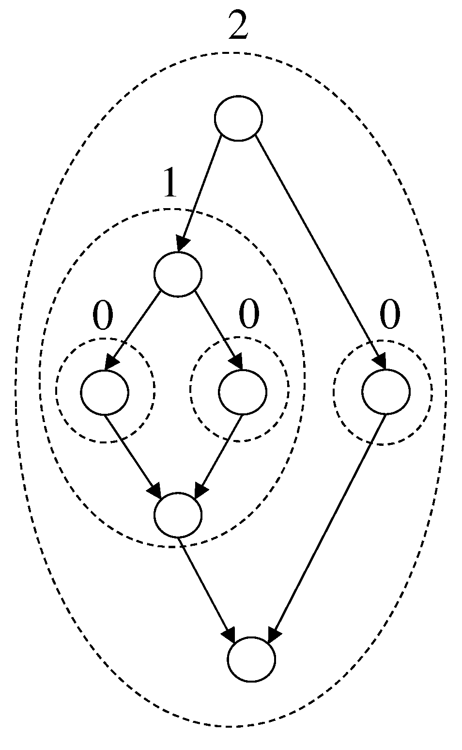
Each edge is called a top edge of G and each edge is called a bottom edge of G. An FJ-DAG has a nested structure. We introduce the level of an FJ-DAG G, denoted by , as follows: (i) the level of a single vertex G is 0; (ii) if are children of G, then . Any FJ-DAG contained in an FJ-DAG G as a subgraph is called a sub FJ-DAG of G. Figure 1 shows an FJ-DAG, where the level of each sub FJ-DAG is indicated. We also define the level of each edge. The level of an edge is defined as the level of a sub FJ-DAG that contains the edge as a top or bottom edge. Such a class of graphs is well studied in the research field of queuing networks since it appears in various applications such as parallel computing and flexible manufacturing systems [17].
In an FJ-DAG , a path from to is called a goal path of G. Now, we define a graph problem, Pathfinding in an FJ-DAG with Unknown Edge Length (PFJUEL), as follows:
Given
- An FJ-DAG ;
- Oracle : given two vertices , and a nonnegative integer c, the oracle answers whether the length of edge is less than or equal to c or not.
Assumption
- Each edge has a nonnegative integer length, but the length is unknown in advance and should be found by calling the oracle.
Find
- A shortest goal path.
PFJUEL is an online problem since the length of each edge is known only by calling oracles. As we have mentioned in the introduction, any procedures that solve such an online problem should be adaptive; i.e., the next action (i.e., an oracle call) to be taken is determined by the current knowledge of the target. Such a procedure is called a strategy. Roughly speaking, the objective of PFJUEL is to find a strategy that is optimal for the total cost of oracle calls. The formal statement of an optimal strategy to PFJUEL is given after we introduce the required concepts and terminology.
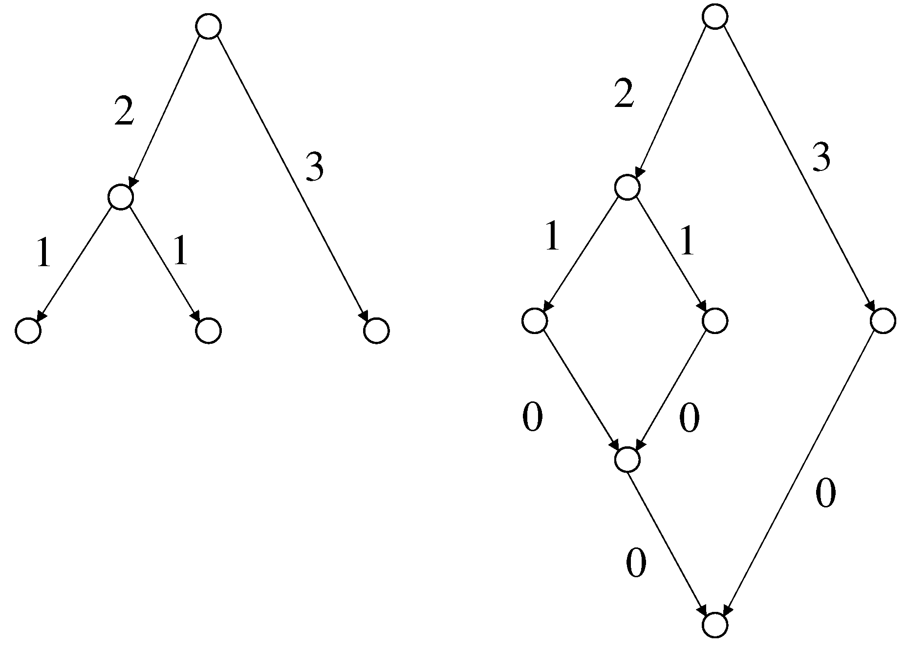
We note that PFJUEL is a generalization of the problem PSTUEL studied in [1]. The targets of PSTUEL are directed trees. Given a directed tree, we can make an FJ-DAG such that the shortest goal path of the FJ-DAG contains the shortest goal path of the directed tree, where a goal path of a tree is a path from the root to a leaf. To do this, we add edges with length 0 so that the tree becomes an FJ-DAG (Figure 2).
At some step of a strategy for PFJUEL, the set of edges E is partitioned into two sets and , where the length of each edge is already known, and the length of each edge in is unknown. An edge moves from to when its length has been found. Moreover, for each edge , a lower bound of the edge length is obtained by previous oracle calls. The initial lower bound is 0, and if returns “no”, then is set to .
Definition 2.
A strategy that does not call for is called conservative.
In conservative strategies, an edge moves from to when returns “yes” for . Since calling the oracle for a large c is dominant in the total computational cost, we concentrate on conservative strategies only. In this class of strategies, calling for all in this order is mandatory to know the correct edge length.
3. Estimate and Characteristic Vector
For conservative strategies, the current knowledge about the graph is represented by a pair , where is the set of all pairs with , and is the set of all pairs with . We call such F an estimate of G. Let denote the set of all estimates. A strategy for PFJUEL is formally defined as a mapping from to (this definition of strategies means that strategies are deterministic; i.e., any strategy gives the same response to the same estimate). Based on the previous results on oracle calls, strategy gives the next edge in and nonnegative integer c for which the oracle is called. The current lower bound of the path length is given by the sum of for all edges on the path. We call this the estimated length of the path.
When a shortest goal path is found, the estimate has to satisfy the following requirements in order to guarantee the correctness of the result.
Definition 3.
An estimate is called terminal if the following two conditions hold:
- R1.
- All the edges on a shortest goal path are in ;
- R2.
- For any goal path other than , its estimated length is no less than the length of .
In what follows, oracle calls that return “no” are called fail calls and oracle calls that return “yes” are called success calls. Given an estimate F, we define a vector called the characteristic vector of F, where each is the number of edges with , and s is the largest integer such that . In conservative strategies, the number of fail calls is given by , because if fails, then fails for all .
To define the optimality of strategies, we introduce a lexicographical order ⪯ on the set of characteristic vectors. For two characteristic vectors and , we write if (i) or (ii) and holds for , and define to be or .
Definition 4.
A terminal estimate F is called optimal if for any other terminal estimate , holds.
The characteristic vectors do not reflect the number of success calls, since the lower bound is not updated for any success call. In the conservative strategies, however, every success call for is preceded by a fail call . This means that the number of success calls is no greater than the number of fail calls . For this reason, the optimality defined above can be a measure of the total computational cost.
We have assumed that the cost of calling oracles is dominant in the total computation time and it becomes exponentially larger as the length c increases. Since we give no exact computational cost of oracle calls, the optimality of a strategy should be defined by the number of oracle calls. Under the assumption of the computational cost of oracle calls, the above definition is reasonable. In our previous paper, we initially intended to use the same evaluation measure as that used in this paper. However, we could not prove the optimality for it and could prove the optimality for a weaker measure in which only the number of oracle calls for the largest c is considered.
If all goal paths have the same estimated length h, then the estimate is called homogeneous with length h.
Lemma 1.
Any optimal estimate is homogeneous.
Proof.
Assume that there exists an optimal estimate having at least one goal path with length , where is the length of the shortest goal path. Choose a goal path with length h. has the form
where denotes the index of a sub FJ-DAG . If does not share edges with any goal path with length , then we choose one edge with a nonzero estimated length (since , such an edge exists) and decrement the estimated length by one. Suppose that shares an edge or with goal paths having length . From the structure of FJ-DAGs, edges , are also shared. Since is longer than such paths with length , there exists an edge or , that is not shared by such goal paths and has a nonzero estimated length. Then, we decrement the estimated length of the edge by one. As a result, the length of can be decreased by one. The estimate is still terminal after this procedure. This contradicts to the assumption that the estimate is optimal. □
4. Canonical Estimate
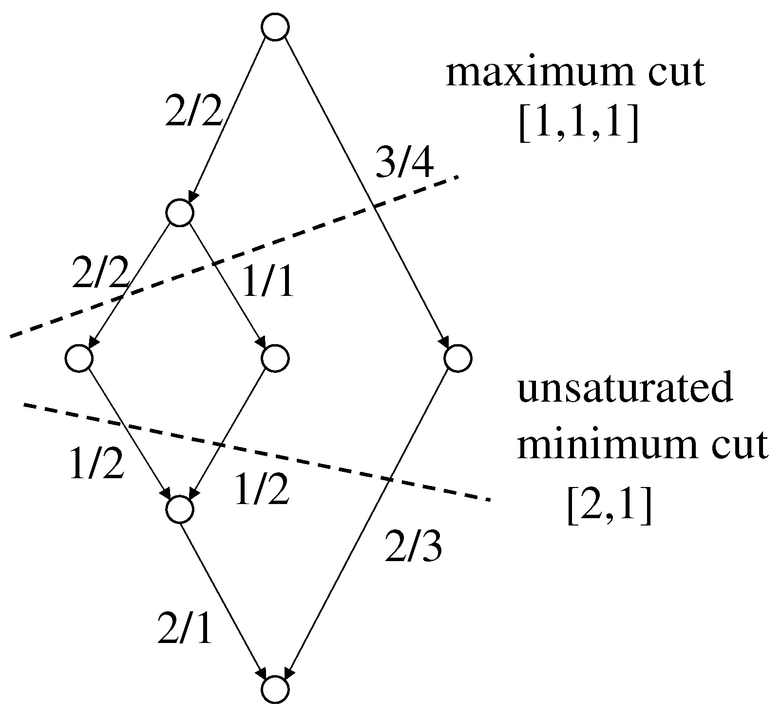
In this section, we introduce a special class of estimates, called canonical estimates, that gives optimal estimates. We first introduce some terminology. An edge is called saturated if , and is called unsaturated if . A cut is a subset of edges such that it contains exactly one edge on every goal path. Let F be the characteristic vector of an estimate. Then, the characteristic vector of a cut is the restriction of F to the edges in the cut. A cut is called maximum if its characteristic vector is maximum with regard to ⪯ in all cuts. A cut is called unsaturated if it consists of unsaturated edges only. An unsaturated minimum cut is an unsaturated cut such that its characteristic vector is minimum with regard to ⪯ in all unsaturated cuts. Figure 3 shows a maximum cut with characteristic vector and an unsaturated minimum cut with characteristic vector [2, 1].
Definition 5.
(Canonical Estimate)
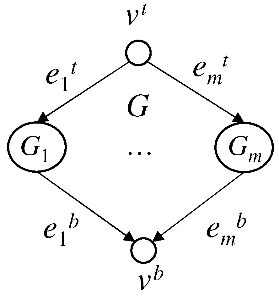
Let F be an estimate of an FJ-DAG G. If , then F is canonical. Suppose that G has children as shown in Figure 4. Then, F is called canonical if it is homogeneous and the following conditions hold for all :
- C1.
- F is canonical for ;
- C2.
- If is unsaturated, then holds;
- C3.
- If and is unsaturated, then holds, where is the largest estimated length in ;
- C4.
- If and has at least one unsaturated cut, then and hold, where is the largest estimated length in all unsaturated minimum cuts of .
Since any canonical estimate is homogeneous, all goal paths have the same estimated length. We take a canonical estimate with length h to indicate that the estimated length is h.
By reassigning the estimated lengths of some edges, the characteristic vector of a non-canonical estimate may decrease without changing its length. We show examples. The estimate shown in Figure 5a does not satisfy C2. By the reassignment shown in Figure 5b, the characteristic vector decreases. The estimate shown in Figure 6a does not satisfy C3 because the maximum estimated length of the sub FJ-DAG is 6, which is greater than the value of 3 of the bottom edge. As shown in Figure 6b, the characteristic vector decreases by adding one to the bottom edge and removing one from every edge on the maximum cut. The estimate shown in Figure 7a does not satisfy C4 because the maximum estimated length on the unsaturated minimum cut of the sub FJ-DAG is 4, and 4 + 1 = 5 is less than the value of 6 of the bottom edge. As shown in Figure 7b, the characteristic vector decreases by removing one from the bottom edge and adding one to every edge on the unsaturated minimum cut. These operations are used to prove the optimality of canonical estimates.
Lemma 2.
Let G be an FJ-DAG shown in Figure 4, and let F be a canonical estimate for G with length h. Then, for each , and are unique up to their exchange.
Proof.
We first consider the case that . Then, holds. If both and are saturated, then the value assignment is unique. If both and are unsaturated, then by C2, holds and the value assignment to these edges are unique up to exchange of them. Suppose that is saturated and is unsaturated. Then, by C2, holds. If , then this is the unique assignment to these two edges. If , then we can obtain another assignment by decrementing by one and incrementing by one. No other assignments are possible. Therefore, the value assignment is unique up to their exchange. This also holds for the case that is unsaturated and is saturated.
Next, we consider the case that . Suppose that has no unsaturated cut. Then, has a goal path with saturated edges only. Let be the length of such a saturated goal path. Note that is uniquely determined, and all goal paths of have the same estimated length since F is homogeneous. Therefore, is also unique. By the same argument as in the case , we can prove the lemma.
Suppose that has at least one unsaturated cut. Let (x is t or b) be an unsaturated edge in such that it is on a minimum unsaturated cut C of and . Let be the sub FJ-DAG having as the top or bottom edge. By C3, every edge in is with an estimated length no greater than . We claim that has a goal path such that all unsaturated edges on the path are with estimated length . Assume that has no such goal paths. Then, has an unsaturated cut with a characteristic vector smaller than that of . By replacing with in the cut C, we obtain an unsaturated cut of with a smaller characteristic vector than C, which is a contradiction. Since is homogeneous, any goal path in has the same estimated length, and it is uniquely determined.
Let be a goal path that goes through . has the form
where and . Note that subpaths and are uniquely identified. We consider the case that x is t. The case that x is b is similarly proved. We make the following observations:
- The estimated length of the subpathin is uniquely determined; [by the fact that F gives the unique estimated length to goal paths of as shown above]
- if ; otherwise; [by the fact that is on a minimum unsaturated cut of (This exclude that case ), as we have assumed, and C2]
- if ; otherwise (x is t or b, ); [by C3 and C4]
- if is unsaturated (x is t or b, ). [by C3]
The estimate for and that satisfies the above properties is obtained by the following procedure.
- 1.
- Assign to if ; otherwise, make saturated (x is t or b, );
- 2.
- At this moment, the current estimate is the minimum estimate that satisfies all the properties. If the length of is h, then halt;
- 3.
- From outmost unsaturated edges and , increment the estimated length by one until the length of reaches h.
Figure 8 shows an estimate obtained by this procedure, where . When the procedure terminates, and are unique up to their exchange. □
Proposition 1.
Let G be an FJ-DAG. Any canonical estimate for G with length h has the same characteristic vector.
Proof.
Let F be a canonical estimate for G, as shown in Figure 4. The proposition is obvious when . Suppose that . We can consider each i separately. By Lemma 2, and are unique up to their exchange. Therefore, the length of F in is also the same in any canonical estimate. By the induction hypothesis, any canonical estimate for has the same characteristic vector, and therefore any canonical estimate for G has the same characteristic vector as well. □
Lemma 3.
Let F be any homogeneous estimate for G with length h. Then, there exists a canonical estimate with the same length h and .
Proof.
If a homogeneous estimate is not canonical, then at least one of C2, C3, and C4 is not true in some sub FJ-DAG of G. We introduce procedures to make the estimate canonical.
Violation of C2: Let be a sub FJ-DAG in which C2 is false. This means that () is unsaturated and (). Then, increment () by one and decrement () by one (see Figure 5).
The following holds:
- The estimate is still homogeneous with the same length after the update;
- By repeating this procedure, C2 eventually becomes true in ;
- The characteristic vector decreases after the update;
- If C2 is true in another sub FJ-DAG of G, then C2 is still true in after the update.
Violation of C3: We assume C2 is true in any sub FJ-DAG. Let be a sub FJ-DAG in which C3 is false. Then, () is unsaturated and (). Choose a maximum cut of . Then, the cut contains an edge with estimated length . We claim that every edge on this cut has a positive estimated length. This is proved as follows. Assume that the cut has an estimated length of 0. Since the cut is maximum, there exists a sub FJ-DAG of with top and bottom edges in which all edges have an estimated length of 0 (the minimal case is a single vertex with top and bottom edges). Let be a maximal such sub FJ-DAG of . since has an edge with a positive estimated length. Then, there exists a sub FJ-DAG of that shares top and bottom vertices with and has a positive length. This contradicts the assumption that F is homogeneous.
Decrement the estimated length of every edge on the cut by one. If () is saturated and () is unsaturated, then increment () by one. If both and are unsaturated, then increment or by one if ; increment by one if ; increment by one if (see Figure 6).
The following holds:
- The estimate is still homogeneous with the same length after the update;
- By repeating this procedure, C3 eventually becomes true in ;
- If has more than one children, then the characteristic vector decreases after the update. If has only one child, then the characteristic vector decreases or does not change after the update;
- If C2 is true in a sub FJ-DAG of G, then C2 is still true in after the update. This is because the decrement is applied to edges on the maximum cut, and the increment is applied in such a way that C2 still holds;
- may decrease in some FJ-DAG of G. This change does not make C3 false in any sub FJ-DAG.
Violation of C4: We assume C2 and C3 are true in any sub FJ-DAG. Let be a sub FJ-DAG in which C4 is false. Then, or holds. Choose an unsaturated minimum cut of . Increment every edge on the cut by one. Decrement or by one if ; decrement by one if ; decrement by one if (see Figure 7).
The following holds:
- The estimate is still homogeneous with the same length after the update;
- By repeating this procedure, C4 eventually becomes true in ;
- The characteristic vector decreases after the update;
- If C2 is true in a sub FJ-DAG of G, then C2 is still true in after the update. This is because the increment is applied to edges on the minimum cut, and the decrement is applied in such a way that C2 still holds;
- may decrease in some FJ-DAG of G. This change does not make C3 false in any sub FJ-DAG;
- may increase in some FJ-DAG of G. This change does not make C4 false in any sub FJ-DAG;
- When , increases and C3 may become false. We show that this does not happen. Since C3 is true in before the update, () holds if () is unsaturated. Suppose that is updated. By the procedure, holds before the update. If is saturated, then C3 is still true after the update. Suppose that is unsaturated. Then, holds by C2. Since before the update, holds after the update. Moreover, holds before the update, and therefore holds after the update. Hence, C3 is still true in even when is incremented by one. This also holds when is updated.
By applying these procedures, we eventually obtain a canonical estimate with the same length such that . □
By Proposition 1 and Lemma 3, we have the following theorem that characterizes the optimal estimates.
Theorem 1.
The characteristic vector of any canonical estimate with length h is minimum with regard to ⪯ in all homogeneous estimates with length h.
Using Lemma 1, we have the following corollary.
Corollary 1.
Let F is a terminal estimate for an FJ-DAG G. If F is canonical, then it is optimal.
5. A Solution to PFJUEL
In this section, we present a solution method to PFJUEL that gives a canonical estimate for FJ-DAGs. It is a strategy defined as follows Algorithm 1:
| Algorithm 1:Shortest Path Increment from Outmost Edges (SPIOE): |
|
Remark 1.
At line 12, there may be more than one edge in . To make the strategy deterministic, we need some rule to select one edge; e.g., introducing a total order to the set of edges.
Let be the length of a shortest goal path. Suppose that an edge is selected in the while loop, and is on a goal path whose estimated length already reaches . If , then returns “no” and the estimated length of becomes . Such an oracle call is unnecessary for satisfying the requirement R2. We call such a fail call a waste fail call. Waste fail calls are unavoidable if the length of each edge is initially unknown.
Lemma 4.
If waste fail calls do not occur, then the estimate given by SPIOE is canonical.
Proof.
If the oracle call is not a success call, then SPIOE increments the length of a goal path with the shortest estimated length by one. Since waste fail calls do not occur, the estimated length of every goal path does not exceed the length of the shortest goal path, and therefore SPIOE gives a homogeneous estimate when it terminates.
We show that the violation of C2–C4 does not occur in any sub FJ-DAG during the execution of SPIOE. This is proved by mathematical induction in the number of iterations. Initially, the estimate is canonical.
Assume that the current estimate satisfies C2–C4 in any sub FJ-DAG. Suppose that the estimated length of the upper edge of a sub FJ-DAG has been updated; i.e., incremented by one.
We first show that C2–C4 still hold in after the update.
C2: If is saturated just before the update, then a violation of C2 does not occur. Suppose that is unsaturated just before the update. Note that every goal path that contains also contains . Then, by line 7, holds just before the update. Therefore, C2 is still true after the update.
C3: Since holds just before the update, then C3 is still true after the update.
C4: If just before the update, then C4 is still true after the update. Suppose that just before the update. Any goal path that contains also contains an edge in a minimum unsaturated cut of . Then, the path contains an unsaturated edge with an estimated length no greater than . By line 7, SPIOE does not choose because is not minimum in unsaturated edges on the path.
The case that has been updated is similar. Next, we show that C2–C4 are still true in other sub FJ-DAGs after the update. Since C2 is the condition for the top and the bottom edge of each sub FJ-DAG, C2 is still true in any sub FJ-DAG after the update. In any sub FJ-DAG that does not contain , C3 and C4 are still true after the update. Thus, we need to check the conditions for sub FJ-DAGs that contain . Let be such a sub FJ-DAG. Then, and may be incremented by one. Suppose that is incremented. This occurs when just before the update. C3 becomes false after the update only if for the top or bottom edge of , holds just before the update. Every goal path that contains also contains because is in a level higher that that of . Therefore, SPIOE does not choose by line 10, and this case does not occur. Clearly, C4 is still true when is incremented. Thus, C3 and C4 are still true in other sub FJ-DAGs.
By the above arguments, C2–C4 are still true in all sub FJ-DAGs after the update. Hence, we can conclude that the obtained estimate is canonical. □
Remark 2.
The condition at line 4–5 is not used in the above proof. Dropping this condition may cause waste fail calls and unnecessary success calls.
From Corollary 1 and Lemma 4, we obtain the main theorem.
Theorem 2.
If waste fail calls do not occur, then SPIOE always gives an optimal estimate.
The detailed complexity analysis of the SPIOE is omitted for the following reasons. The analysis can be done for (i) the characteristic vector of the optimal terminal estimate obtained by SPIOE and (ii) the total computational time of SPIOE. The optimal terminal estimate is characterized by Corollary 1 (i.e., canonical estimate) and is determined by the given FJ-DAG. It may be possible to give trivial lower/upper bounds of the characteristic vector, but they are meaningless. The total computational time of SPIOE is obtained by evaluating operations in each iteration and the total number of iterations. Operations in each iteration consist of maintaining shortest goal paths and finding an edge with the minimum estimated length in the highest level. They can be done in polynomial time. Furthermore, we can give an upper bound of the number of iterations, which is determined by the optimal terminal estimates. This is apparently polynomial in the size of the graph and edge length. Such detailed complexity analysis is not very valuable under the above cost assumption on calling oracles. Moreover, the goal of the paper is to develop an optimal strategy that can be applied to real problems. In this sense, the goal has been achieved.
Finally, we analyze the number of waste fail calls. Let be the length of the shortest goal path. We introduce a special class of strategies. Strategies that always issue oracle calls to unsaturated goal paths with the shortest estimated length are called rational. In the terminal estimate obtained by any rational strategy, the estimated length of every goal path is always less than or equal to , and therefore the number of waste fail calls is less than the number of goal paths.
Lemma 5.
Let g be the number of goal paths. Then, is an upper bound of the number of waste fail calls by any rational strategy.
For a strategy that is not rational, the estimated length of some goal path may become greater than . Suppose that the estimated length of the current shortest goal path has reached and the strategy issues an oracle call to a goal path with length . We can make an instance of FJ-DAGs for which the oracle call fails and the estimated length becomes .
There exists an FJ-DAG for which any rational strategy gives waste fail calls; i.e., is the tight upper bound for rational strategies. Let us consider an FJ-DAG shown in Figure 9, where every edge has length 1. At each round, any rational strategy picks up one unsaturated edge on a goal path with the shortest estimated length and issues an oracle call to it. Then, we will eventually reach the following situation: all edges are saturated but are in . The next oracle call is issued to some edge and it succeeds. Then, we consider an instance having a length of 2 for this edge. The strategy shows the same behavior for the new instance before this oracle call, but now the oracle call fails. Since the strategy is rational, the next oracle call is issued to an edge on a goal path with an estimated length of 2. We can repeat this times. After that, we obtain a goal path with a length of 2 such that all edges on it are in . When a terminal estimate is obtained, the number of waste fail calls issued so far is . Hence, we have the following result.
Lemma 6.
Given any rational strategy, there is an instance of FJ-DAGs for which the the number of waste fail calls is , where g is the number of goal paths.
We demonstrate the execution of strategy SPIOE. Consider an FJ-DAG in Figure 10a. The obtained terminal estimate by SPIOE is shown in Figure 10b. Bold arrows indicate that success calls occur at the edges. The shortest goal path is .
The execution trace is shown in Table 1, where each column indicates the estimated length of the current shortest goal path, the number c and the edge in oracle call , and the result. In this trace, no waste fail calls occur.
6. Conclusions
We have studied a pathfinding problem of FJ-DAGs with unknown edge length and have proposed a strategy that gives a shortest path. The strategy is optimal in the sense that the characteristic vector consisting of the number of fail oracle calls for each length is minimized with respect to a lexicographical order, provided that there are no waste fail calls. Theoretical upper bounds on the number of waste fail calls are also given. As a result, several technical problems that remained in the previous paper have been solved; i.e., showing optimality for a stronger criterion, which was initially intended to use in the previous paper, and making the discussion clearer.
Although PFJUEL is a purely theoretical problem, solution methods for it can contribute to reducing the cost of configuration change in reconfigurable cloud computing systems. The proposed strategy is an optimal one under a reasonable assumption; i.e., no other strategy is better than this. This is a notable result. Extending the targets to graphs with cycles remains as future work. In real applications, if the upper bound of the edge length is known, then the average computational cost may be reduced by non-conservative strategies. This issue should be also studied in the future.
Funding
This research received no external funding.
Institutional Review Board Statement
Not applicable.
Informed Consent Statement
Not applicable.
Conflicts of Interest
The author declares no conflict of interest.
References
- Hiraishi, K.; Kobayashi, K. A Pathfinding Problem for Search Trees with Unknown Edge Length. J. Discret. Algorithms 2018, 49, 1–7. [Google Scholar] [CrossRef]
- Kikuchi, S.; Tsuchiya, S. Configuration Procedure Synthesis for Complex Systems Using Model Finder. In Proceedings of the 15th IEEE International Conference on Engineering of Complex Computer Systems (ICECCS 2010), Oxford, UK, 22–26 March 2010; pp. 95–104. [Google Scholar]
- Kikuchi, S.; Tsuchiya, S.; Hiraishi, K. Synthesis of Configuration Change Procedure Using Model Finder. IEICE Trans. Inf. Syst. 2013, E-96-D, 1696–1706. [Google Scholar] [CrossRef] [Green Version]
- Hart, P.E.; Nilsson, N.J.; Raphael, B. A Formal Basis for the Heuristic Determination of Minimum Cost Paths. IEEE Trans. Syst. Sci. Cybern. 1968, 4, 100–107. [Google Scholar] [CrossRef]
- Korf, R. Depth-first Iterative-Deepening: An Optimal Admissible Tree Search. Artif. Intell. 1985, 27, 97–109. [Google Scholar] [CrossRef]
- Björnsson, Y.; Enzenberger, M.; Holte, R.C.; Schaeffer, J. Fringe Search: Beating A* at Pathfinding on Game Maps. In Proceedings of the 2005 IEEE Symposium on Computational Intelligence and Games, Colchester, Essex, UK, 4–6 April 2005; pp. 125–132. [Google Scholar]
- Russell, S. Efficient Memory-bounded Search Methods. In Proceedings of the 10th European Conference on Artificial Intelligence, Vienna, Austria, 3–7 August 1992; pp. 1–5. [Google Scholar]
- Nikolova, E.; Kelner, J.A.; Brand, M.; Mitzenmacher, M. Stochastic Shortest Paths via Quasi-convex Maximization. Theor. Comput. Sci. 2006, 4168, 552–563. [Google Scholar]
- Papadimitriou, C.H.; Yannakakis, M. Shortest Paths Without a Map. In Lecture Notes in Computer Science; (Proc. 16th ICALP); Springer: Berlin/Heidelberg, Germany, 1989; Volume 372, pp. 610–620. [Google Scholar]
- Karger, D.; Nikolova, E. Exact Algorithms for the Canadian Traveler Problem on Paths and Trees; MIT CSAIL Technical Report; MIT: Cambridge, MA, USA, 2008; MIT-CSAIL-TR-2008-004. [Google Scholar]
- Gyögy, A.; Linder, T.; Lugosi, G.; Ottucsák, G. The On-Line Shortest Path Problem Under Partial Monitoring. J. Mach. Learn. Res. 2007, 8, 2369–2403. [Google Scholar]
- Khani, A. An Online Shortest Path Algorithm for Reliable Routing in Schedule-based Transit Networks Considering Transfer Failure Probability. Transp. Res. Part B 2019, 126, 549–564. [Google Scholar] [CrossRef]
- Blei, D.; Kaelbling, L. Shortest Paths in a Dynamic Uncertain Domain. In Proceedings of the IJCAI Workshop on Adaptive Spatial Representations of Dynamic Environments, Stockholm, Sweden, 31 July–2 August 1999. [Google Scholar]
- Boyan, J.; Mitzenmacher, M. Improved Results for Route Planning in Stochastic Transportation Networks. In Proceedings of the Twelfth Annual ACM-SIAM Symposium on Discrete Algorithms, Washington, DC, USA, 7–9 July 2001; pp. 895–902. [Google Scholar]
- Nikolova, E.; Brand, M.; Karger, D.R. Optimal Route Planning Under Uncertainty. In Proceedings of the International Conference on Automated Planning and Scheduling, Cumbria, UK, 6–10 June 2006; pp. 131–140. [Google Scholar]
- Karp, R.M. On-Line Algorithms Versus Off-Line Algorithms: How Much is it Worth to Know the Future? In Proceedings of the IFIP 12th World Computer Congress on Algorithms, Software, Architecture-Information Processing ’92, Madrid, Spain, 7–11 September 1992; Volume 1, pp. 416–429. [Google Scholar]
- Baccelli, F.; Massey, W.A.; Towsley, A. Acyclic Fork-join Queuing Networks. J. ACM 1989, 36, 615–642. [Google Scholar] [CrossRef]
Figure 1.
An FJ-DAG. The level of each sub FJ-DAG is indicated.

Figure 2.
A tree and the constructed FJ-DAG.

Figure 3.
Maximum/minimum cut (for each edge , is indicated).

Figure 4.
Structure of FJ-DAG.

Figure 5.
Reassignment for violation of C2: (a) before the reassignment, (b) after the reassignment (for each edge , is indicated).
Figure 5.
Reassignment for violation of C2: (a) before the reassignment, (b) after the reassignment (for each edge , is indicated).

Figure 6.
Reassignment for violation of C3: (a) before the reassignment, (b) after the reassignment (for each edge , is indicated).
Figure 6.
Reassignment for violation of C3: (a) before the reassignment, (b) after the reassignment (for each edge , is indicated).

Figure 7.
Reassignment for violation of C4: (a) before the reassignment, (b) after the reassignment (for each edge , is indicated).
Figure 7.
Reassignment for violation of C4: (a) before the reassignment, (b) after the reassignment (for each edge , is indicated).

Figure 8.
A canonical estimate obtained by the procedure.

Figure 9.
An FJ-DAG that gives waste fail calls.

Figure 10.
(a) An FJ-DAG and (b) an optimal estimate.


Table 1.
An execution trace of SPIOE.
| Step | Length | c | Edge | Result |
|---|---|---|---|---|
| 1 | 0 | 0 | (6, 7) | no |
| 2 | 0 | 0 | (1, 5) | no |
| 3 | 1 | 0 | (1, 2) | no |
| 4 | 1 | 0 | (5, 7) | no |
| 5 | 2 | 0 | (2, 3) | no |
| 6 | 2 | 0 | (2, 4) | no |
| 7 | 2 | 1 | (5, 7) | no |
| 8 | 3 | 0 | (3, 6) | no |
| 9 | 3 | 0 | (4, 6) | no |
| 10 | 3 | 1 | (1, 5) | no |
| 11 | 4 | 1 | (1, 2) | no |
| 12 | 4 | 2 | (5, 7) | no |
| 13 | 5 | 1 | (6, 7) | yes |
| 14 | 5 | 1 | (3, 6) | yes |
| 15 | 5 | 1 | (2, 3) | yes |
| 16 | 5 | 2 | (1, 2) | yes |
Publisher’s Note: MDPI stays neutral with regard to jurisdictional claims in published maps and institutional affiliations. |
© 2021 by the author. Licensee MDPI, Basel, Switzerland. This article is an open access article distributed under the terms and conditions of the Creative Commons Attribution (CC BY) license (https://creativecommons.org/licenses/by/4.0/).
Share and Cite
MDPI and ACS Style
Hiraishi, K. A Pathfinding Problem for Fork-Join Directed Acyclic Graphs with Unknown Edge Length. Algorithms 2021, 14, 367. https://0-doi-org.brum.beds.ac.uk/10.3390/a14120367
AMA Style
Hiraishi K. A Pathfinding Problem for Fork-Join Directed Acyclic Graphs with Unknown Edge Length. Algorithms. 2021; 14(12):367. https://0-doi-org.brum.beds.ac.uk/10.3390/a14120367
Chicago/Turabian StyleHiraishi, Kunihiko. 2021. "A Pathfinding Problem for Fork-Join Directed Acyclic Graphs with Unknown Edge Length" Algorithms 14, no. 12: 367. https://0-doi-org.brum.beds.ac.uk/10.3390/a14120367
Note that from the first issue of 2016, this journal uses article numbers instead of page numbers. See further details here.