
Fault Diagnosis Algorithm Based on Adjustable Nonlinear PI State Observer and Its Application in UAV Fault Diagnosis

1
School of Mathematics and Big Data, Foshan University, Foshan 528225, China
2
College of Liberal Arts and Sciences, National University of Defense Technology, Changsha 410073, China
3
Hi-Tech Research Institute, Hunan Institute of Traffic Engineering, Hengyang 421099, China
*
Author to whom correspondence should be addressed.
Algorithms 2021, 14(4), 119; https://0-doi-org.brum.beds.ac.uk/10.3390/a14040119
Submission received: 19 March 2021
/
Revised: 7 April 2021
/
Accepted: 7 April 2021
/
Published: 8 April 2021
(This article belongs to the Section Algorithms for Multidisciplinary Applications)
Abstract
:Aiming at the problem of fault diagnosis in continuous time systems, a kind of fault diagnosis algorithm based on adaptive nonlinear proportional integral (PI) observer, which can realize the effective fault identification, is studied in this paper. Firstly, the stability and stability conditions of fault diagnosis method based on the PI observer are analyzed, and the upper bound of the fault estimation error is given. Secondly, the fault diagnosis algorithm based on adjustable nonlinear PI observer is designed and constructed, it is analyzed and we proved that the upper bound of fault estimation under this algorithm is better than that of the traditional method. Finally, the L-1011 unmanned aerial vehicle (UAV) is taken as the experimental object for numerical simulation, and the fault diagnosis method based on adaptive observer factor achieves faster response speed and more accurate fault identification results.
1. Introduction
In the field of industrial control, it is often necessary to estimate the system state on-line and control it according to the estimated state, however, the existence of faults will make the control more difficult. Usually, fault detection, isolation and estimation are three major tasks of fault diagnosis. Compared with fault detection and isolation, fault estimation is more difficult and more significant. Because fault estimation is often the key link of fault-tolerant control and fault regulation system, the quality of fault estimation directly affects the control accuracy and the control performance of the whole system. At present, researchers have done a lot of research on fault diagnosis methods, including data-based fault diagnosis algorithm and model-based fault diagnosis algorithm [1].
- Fault diagnosis algorithm based on dataThe data-based fault diagnosis algorithm mainly uses statistical methods to obtain the characteristics of the data, and constructs the detection threshold through statistics to diagnose the fault. Furthermore, some intelligent algorithms, such as support vector machine (SVM), K-nearest neighbor (KNN) and so on, are also used in fault diagnosis [2,3]. However, most of the data-based fault diagnosis methods are used for fault detection and identification, and it is difficult to estimate the fault amplitude.
- Model based fault diagnosis algorithmThe model-based fault diagnosis algorithm usually needs to accurately model the diagnosis object [4], and obtain the system state by comparing the reference model output with the actual output, so as to judge whether there is a fault in the system [5]. Although this method has high accuracy and reliability, it often takes a lot of energy to accurately model the diagnosis object.
Due to the unmanned aerial vehicle (UAV) control system requires high reliability, it needs more accurate fault diagnosis algorithm [6]. The data-based fault diagnosis algorithm is not suitable for UAV control system because of its low accuracy and inability to estimate fault effectively [7]. On the contrary, a large number of scholars have conducted in-depth research on UAV control system and established perfect mathematical and physical models [8]. Therefore, the model-based fault diagnosis algorithm can provide highly reliable fault diagnosis results for UAV control system. A large number of scholars have studied the model-based UAV fault diagnosis method.
The proportional integral (PI) control algorithm is the most widely used control algorithm. It mainly considers the historical information, current information and future information of dynamic system output error to construct state observer to realize the state and fault monitoring. In References [9,10], the method of fault detection observer was first proposed. Its basic idea is to detect the fault of linear system by designing fault detection observer. In Reference [11], a set of structured residuals is proposed, in which each residuals is only sensitive to some faults but not to others. In Reference [12], the observer based method is deeply studied, and an improved PI observer based on adaptive gain scheduling method and its design method are proposed. In addition, in References [13,14], the parameter estimation problem of PI observer was considered, and the optimal planning algorithm for determining the optimal parameters was designed. In the simulation, the overshoot of fault estimation process was obviously reduced, and the robustness of PI control system was effectively improved. In References [15,16,17], a fault estimation method based on PI observer and considering imprecise scheduling parameters is proposed for a class of nonlinear systems described by linear variable parameter mathematical model.
Most UAV fault diagnosis algorithms are based on PI control algorithm. In References [18,19], a widely applicable fault estimation observer was designed by the optimization technology for the UAV system with an actuator fault and sensor fault. However, due to the existence of constraints, the upper bound of fault estimation error was related to the parameters. In References [20,21], an active fault-tolerant control algorithm based on the interpolation gain scheduling PI was proposed for the actuator fault of the UAV. It was verified on the UAV experimental platform. The test results showed that the active fault-tolerant control algorithm based on the interpolation gain scheduling PI can effectively improve the fault-tolerant performance of UAV, compared with the simple PID controller. In References [22,23], the robust linear variable parameter observer is applied to the rotating subsystem to detect actuator fault of the UAV. Numerical experiments show the effectiveness of the method. In Reference [24], the problem of distributed fault detection and isolation is studied, and a local fault diagnosis algorithm is designed for each unit of UAV through the linear model. This algorithm is effective in most of common fault situations.
In past research, the linear algorithm of state estimation was widely used. Although this method has advantages in hardware implementation, there is a contradiction between the tracking time and the tracking effect in the performance. In this regard, a nonlinear state estimation algorithm can effectively improve the tracking effect and fundamentally solve the contradiction between the tracking time and the tracking effect.
In this paper, fault diagnosis algorithms based on the nonlinear observer is used to improve the effect of the additive single sensor fault estimation. The adaptive parameter updating algorithm is given, which effectively improves the fault estimation effect. This paper is organized as follows. In the Section 2, the system model and the fault diagnosis algorithm based on the PI state observer are introduced. In the Section 3, the fault estimation of the nonlinear state observer is analyzed. In the Section 4, combined with the UAV system, the simulation verification is carried out, and the fault estimation effect is expected.
2. System Model and PI State Observer
Most control systems are highly complex and nonlinear, and they always have the following form
The usual method is to linearize the system near the working point of the system. So that, the linear system is as follows
For this reason, the general linear continuous time system is considered
where is the state vector, is the input vector, is the output vector, are the known matrices of the appropriate dimensions, is the unknown fault vector and are the noise vectors.
Remark: It is a reasonable assumption that the unknown fault vector in Equation (3) is common in the state equation and the output equation. Because the origin of the fault should be the same, but it has different forms in the state and output, and its different forms are reflected in and .
In the simple case, without the system noise and observation noise, the PI state observer of system is constructed as follows
where is the estimated state, is the estimated fault, is the estimated output, and are the observer gain matrices to be designed.
The error system, consisting of the state estimation error and the fault estimation error , is investigated
In order to organize it into the matrix form, define
The following theorem, in Reference [14], gives the condition of bounded error.
Theorem 1.
Proof.
Consider the Lyapunov function , then is as follows
Further, the performance tracking index is examined.
Thus, the Theorem 1 is proven. □
When there are the system noise and the observation noise , the state observer (4) is considered, then the error system is easily obtained as follows
In order to organize it into the matrix form, define
The Lyapunov function and the performance tracking index are also examined, and it is easy to know that when the linear inequality
holds, the error system equation Equation (10) is bounded. The bound satisfies
3. Nonlinear State Observer
In the previous section, we analyzed the PI state observer of the linear time invariant system, and considered its stability and stability conditions. In this section, based on the comparison theorem, a class of nonlinear state observers with better stability is constructed. Consider the following forms of the observers [25,26,27]
where is the estimated state, is the observer gain matrix, is the estimated fault, is the estimated output and p is the nonlinear observer adjustment parameter. Besides, the has the following form
where ⊙ denotes multiplication by elements.
The error system equation is investigated
For a good state observer, the following two conditions must be satisfied:
- When the error between the estimated state and the system state is large, the state observer can achieve fast tracking;
- When the error between the estimated state and the system state is small, the state observer can achieve stable tracking.
Therefore, it is necessary to design the nonlinear observer factors under different estimation errors.
In order to realize the above two advantages, we can consider the case of large error first. While the is large, can be chosen, so that
Further, it can be easy to get that
According to the comparison theorem, when the condition in Equation (7) is true, from Equation (8), we can obtain the bound that satisfies
Remark: Equation (15) only holds when is large. When is small, choosing may lead to the amplification of the estimation error, and should be considered.
At this point, it is proved that if the original PI observer in Equation (12) is stable, the nonlinear observer in Equation (13) can improve the observation effect by selecting appropriate parameter.
Furthermore, it is a universal method, and a more general nonlinear observer can be considered
4. Numerical Simulation
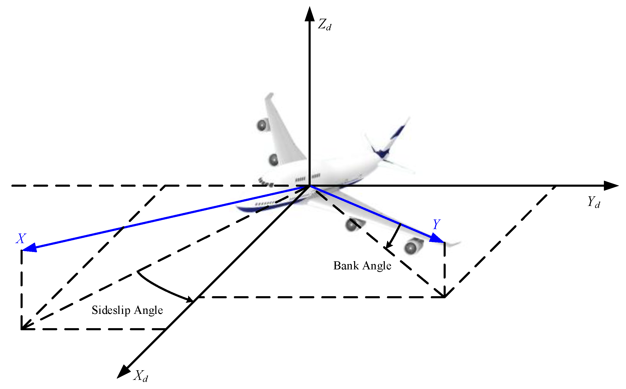
The UAV system is taken as the research object. In Reference [28], based on the detailed modeling of UAV attitude, the classic PI control algorithm is used to control the UAV longitudinal flight attitude. It is proved that the PI control algorithm can make the system track the desired signal better. On the basis of this model, the problem of the sensor fault estimation in UAV system is studied. The attitude model of the UAV is shown in Figure 1.
Accroding to References [29,30,31], the UAV model can be linearized and the system model can be described by Equation (3). The system state is
where are bank angle, roll rate, yaw rate and sideslip angle, respectively.
Its control variable is
where are rudder deflection and aileron deflection, respectively.
Reference [32] shows that, there are two typical failure modes of UAV sensor mechanism:
- Step fault. There is a fixed error between the measured output of the sensor and the actual value of the measured parameter. It is mainly caused by bias current or bias voltage.
- Periodic fault. The error caused by the superposition of the measured output value of the sensor with the signal of a certain frequency. It mainly includes power signal interference and so on.
These two kinds of faults are the main factors that cause UAV to deviate from the course, so we carried out simulation experiments on these two kinds of faults.
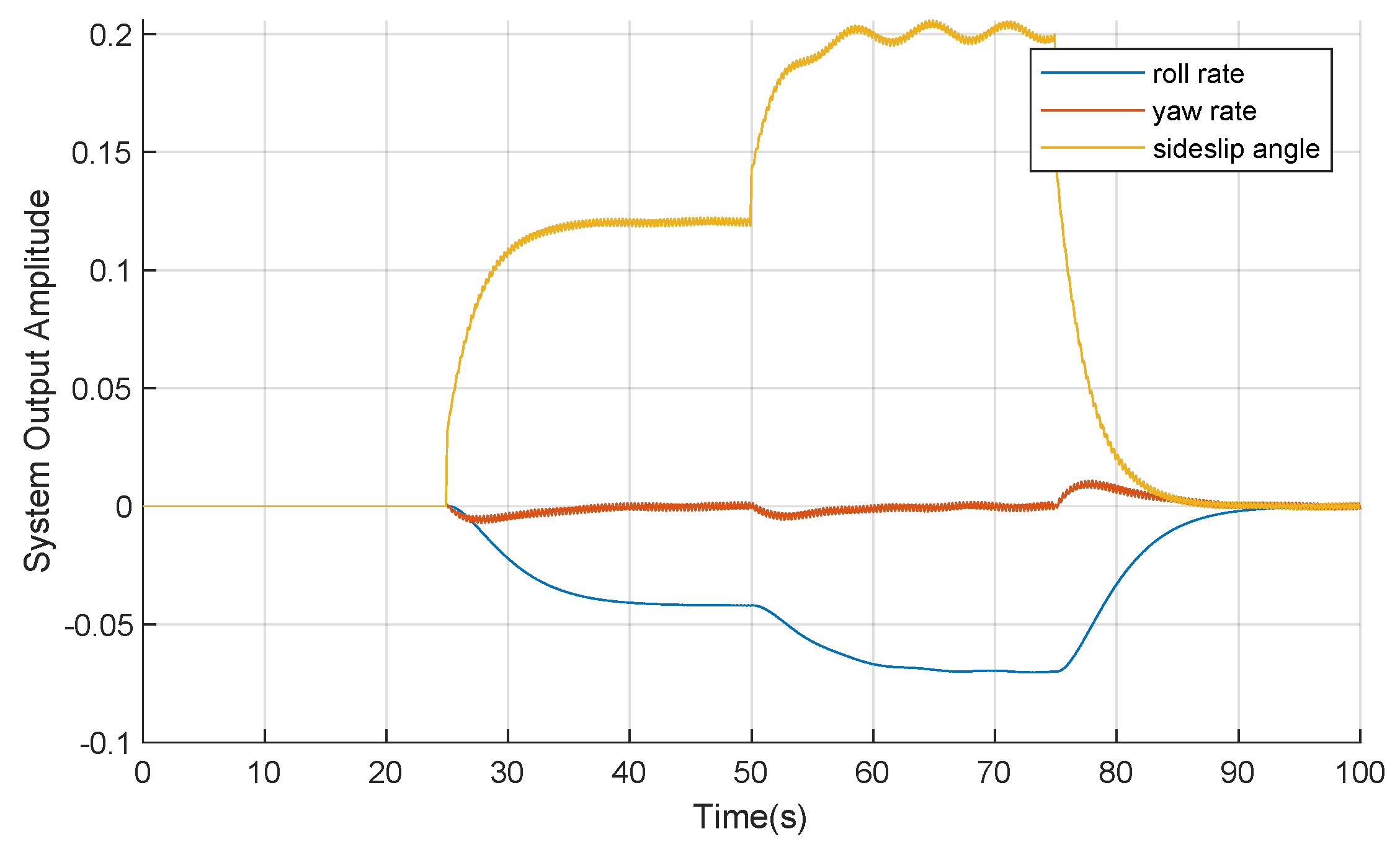
The UAV system works normally in 0 s∼25 s, a step fault with the amplitude occurs in 25 s∼50 s, a periodic fault with the amplitude occurs in 50 s∼75 s, and then the fault ends.
The fault represent fluctuation of voltage, and it has the following forms
The system output is shown in Figure 2.
The state feedback of the system is , and the control gain is taken as follows
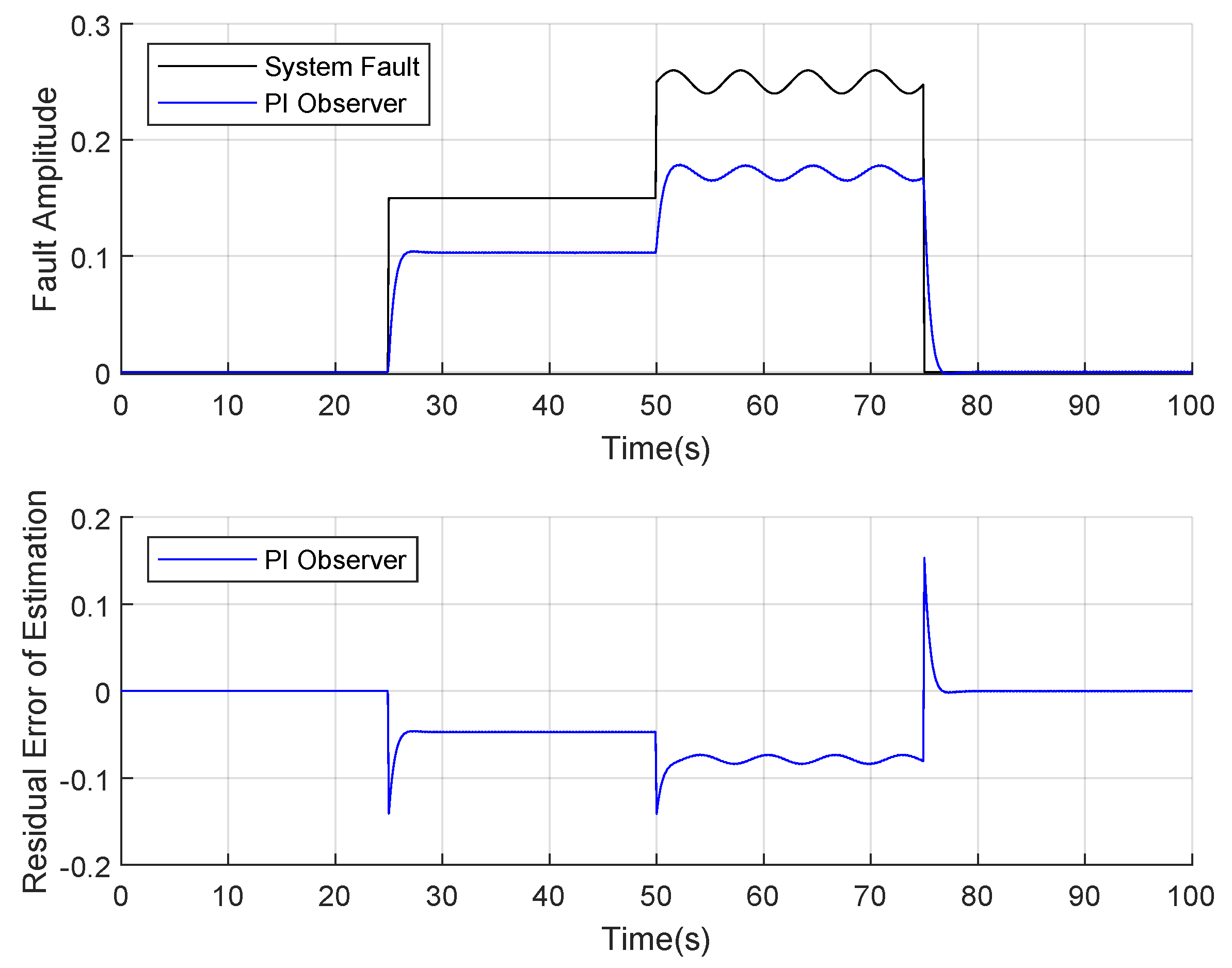
The state observer Equation (4) is adopted, and the fault estimation results are as follows.
It can be seen from Figure 3 that the state observer Equation (4) can track the real fault, but its tracking effect is not ideal. There is a certain deviation from the real fault, and the tracking of the sine function fault has hysteresis.
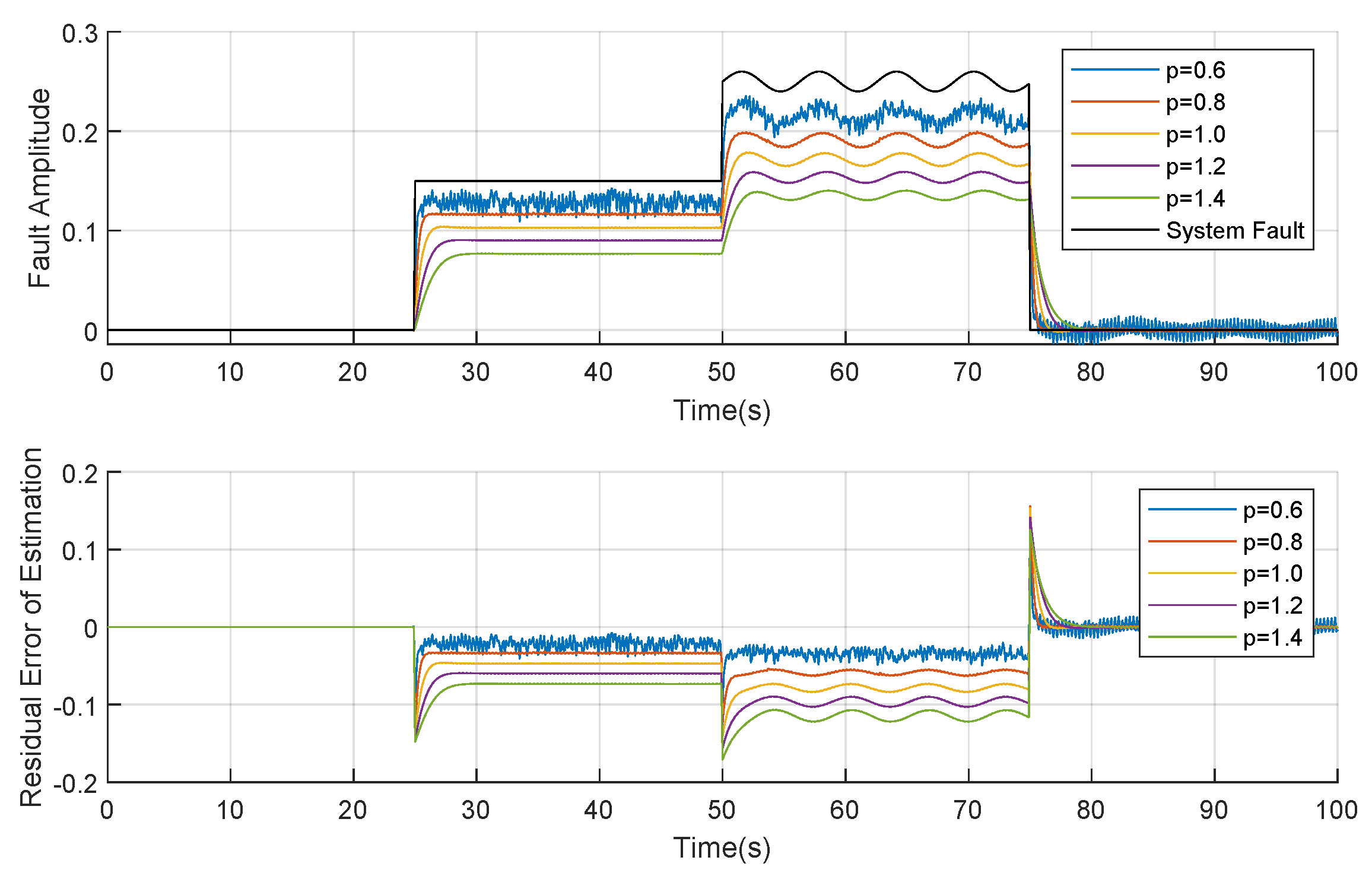
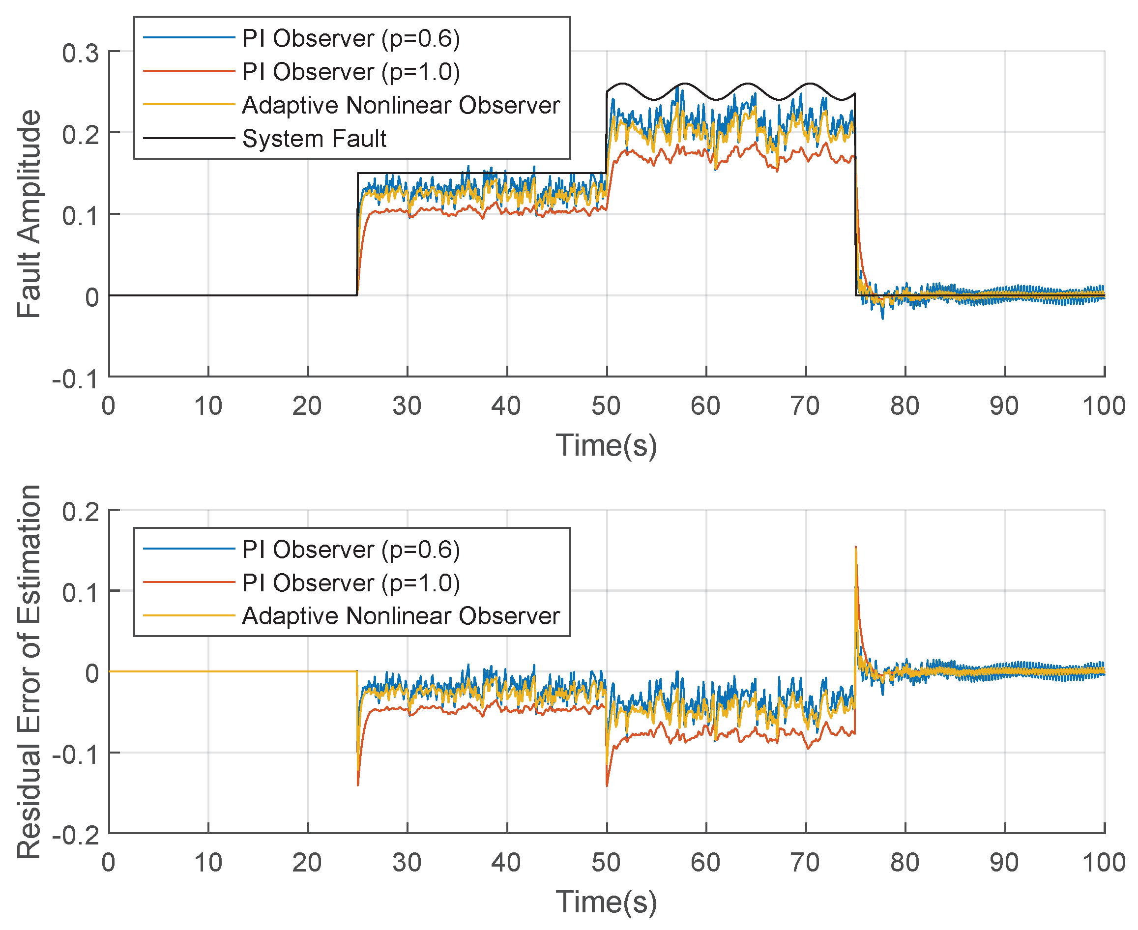
Consider the nonlinear state observer Equation (13), which has the same gain matrix . The fault estimation results are obtained by selecting parameter , respectively. Then, the results are shown in Figure 4.
Obviously, when the difference between the estimated fault and the actual fault is large, the smaller parameter p has a faster response speed, but when the difference becomes small, the larger parameter p has more stable estimation effect. For this reason, according to Equation (15), the adaptive parameter estimation is adopted, which has the faster and more stable tracking effect at the same time.
From Figure 5, we can know that the nonlinear observer with the adaptive parameters combines the stability of the large parameters and the rapidity of the small parameters, which can realize a more reasonable system state estimation. Compared with the PI observer Equation (4), its adjustment time is reduced from s to s, its estimation error for the step fault is reduced from to , and its estimation residual for the periodic fault is reduced from to . Thus it is significantly better than that of the PI observer Equation (4).
When Gaussian noise with mean value of 0 and variance of is added to the system state, the system fault can still be effectively estimated, and the result is shown in Figure 6.
Further, Figure 6 shows that the fault diagnosis algorithm based on adaptive nonlinear PI observer can still achieve better fault estimation effect in the case of system error. Compared with the fault diagnosis algorithm based on linear PI observer, the estimation error is significantly reduced, and the fault estimation result is more robust than that of the fault diagnosis algorithm based on nonlinear PI observer with fixed factor.
5. Conclusions
In this paper, a class of state observers for the linear continuous time systems is discussed, the stability of the state observers, as well as the stability conditions are analyzed and the upper bound of the system error estimation is given. Based on the improvement of the PI state observer, the stability and the stability conditions of the nonlinear state observer are also analyzed, and it is proved that the system state estimation of the nonlinear state observer is better than that of the PI state observer.
In the simulation, the UAV was taken as the simulation object, and the fault estimation effects of the PI state observer and the nonlinear state observer with different parameters were investigated. From the results of the fault estimation, with a large parameter, the fault estimation results are more stable, but the offset between the estimated fault and the real fault is larger. With a small parameter, the estimated faults are closer to the real fault, but there is a large vibration. On this basis, the adaptive parameter selection was investigated. The fault estimation results have smaller offset, faster response speed and smaller vibration amplitude. To sum up, the nonlinear state observer can achieve better track of the system state, and overcome the contradiction between the response and offset in the traditional PI state observer. At the same time, the algorithm can be used to improve other state observers, which can achieve better expansibility.
Although our method has achieved good results in the linear model, there are still some problems to be further studied. Firstly, how to apply this method to the fault diagnosis of nonlinear system and whether it can achieve better fault diagnosis results. Secondly, for the nonlinear system, how to design the corresponding nonlinear observer to improve the effect of fault diagnosis.
Author Contributions
Q.M. proposed the main idea, finished the draft manuscript; J.W. (Juhui Wei) conceived of the experiments and drew the figures and tables; J.W. (Jiongqi Wang) analyzed the data; Y.C. conducted the simulations. All authors have read and agreed to the published version of the manuscript.
Funding
This research is supported by the National Nature Science Foundation of China (No.62001115, 61903086), the Fundamentals and Basic of Applications Research Foundation of Guangdong Province (No.2019A1515110136) and the Project of Department of Education of Guangdong Province (No.2019KTSCX193).
Institutional Review Board Statement
Not applicable.
Informed Consent Statement
Not applicable.
Data Availability Statement
Data sharing not applicable.
Conflicts of Interest
The authors declare no conflict of interest.
References
- Sharma, V. A Review on Vibration-Based Fault Diagnosis Techniques for Wind Turbine Gearboxes Operating Under Nonstationary Conditions. J. Inst. Eng. India Ser. C 2021, 102, 507–523. [Google Scholar] [CrossRef]
- Chen, H.; Jiang, B.; Ding, S.X.; Huang, B. Data-Driven Fault Diagnosis for Traction Systems in High-Speed Trains: A Survey, Challenges, and Perspectives. IEEE Trans. Intell. Transp. Syst. 2020, 50, 1–17. [Google Scholar] [CrossRef]
- Wang, H.; Chai, T.Y.; Ding, J.L.; Brown, M. Data Driven Fault Diagnosis and Fault Tolerant Control: Some Advances and Possible New Directions. Acta Autom. Sin. 2009, 35, 739–747. [Google Scholar] [CrossRef] [Green Version]
- Leonhardt, S.; Ayoubi, M. Methods of fault diagnosis. Control Eng. Pract. 1997, 5, 683–692. [Google Scholar] [CrossRef]
- Saravanakumar, R.; Krishnaraj, N.; Venkatraman, S.; Sivakumar, B.; Prasanna, S.; Shankar, K. Hierarchical symbolic analysis and particle swarm optimization based fault diagnosis model for rotating machineries with deep neural networks. Meas. J. Int. Meas. Confed. 2021, 171, 108771. [Google Scholar] [CrossRef]
- Hui, Y.; Luo, Q.; Yong, L. Application of wavelet and multi-kernel SVM in UAV sensors fault diagnosis. Electron. Meas. Technol. 2014, 37, 112–116. [Google Scholar]
- Guzmán-Rabasa, J.A.; López-Estrada, F.R.; González-Contreras, B.M.; Valencia-Palomo, G.; Chadli, M.; Pérez-Patricio, M. Actuator fault detection and isolation on a quadrotor unmanned aerial vehicle modeled as a linear parameter-varying system. Meas. Control UK 2019, 52. [Google Scholar] [CrossRef] [Green Version]
- Zhong, W.; Xin, C. Fault Detection of UAV Fault Based on a SFUKF. In Proceedings of the IOP Conference Series: Materials Science and Engineering, Bangkok, Thailand, 17–19 May 2019; Volume 563, p. 052099. [Google Scholar] [CrossRef]
- Frank, P.P.R.; Clark, R. Fault Diagnosis in Dynamic Systems: Theory and Applications; Prentice-Hall, Inc.: Hoboken, NJ, USA, 1989; pp. 821–828. [Google Scholar]
- Frank, P.M. Fault diagnosis in dynamic systems using analytical and knowledge-based redundancy. A survey and some new results. Automatica 1990, 26, 450–472. [Google Scholar] [CrossRef]
- Jiang, J. Robust model-based fault diagnosis for dynamic systems. Automatica 2002, 38, 1089–1091. [Google Scholar] [CrossRef]
- Bakhshande, F.; Söffker, D. Proportional-Integral-Observer: A brief survey with special attention to the actual methods using ACC Benchmark. IFAC Pap. 2015, 48, 532–537. [Google Scholar] [CrossRef]
- Boghdady, T.A.; Sayed, M.M.; Emam, A.M.; El-Zahab, E. A Novel Technique for PID Tuning by Linearized Biogeography-Based Optimization. In Proceedings of the IEEE International Conference on Computational Science & Engineering, Porto, Portugal, 21–23 October 2015. [Google Scholar]
- Jiang, B.; Wang, J.L.; Soh, Y.C. An adaptive technique for robust diagnosis of faults with independent effects on system outputs. Int. J. Control 2002, 75, 792–802. [Google Scholar] [CrossRef]
- Ding, S.X.; Li, L.; Krüger, M. Application of randomized algorithms to assessment and design of observer-based fault detection systems. Automatica 2019, 107, 175–182. [Google Scholar] [CrossRef]
- Gómez-Peñate, S.; López-Estrada, F.R.; Valencia-Palomo, G.; Rotondo, D.; Guerrero-Sánchez, M.E. Actuator and sensor fault estimation based on a proportional multiple-integral sliding mode observer for linear parameter varying systems with inexact scheduling parameters. Int. J. Robust Nonlinear Control 2020, 30, 5322–5340. [Google Scholar] [CrossRef]
- Rotondo, D.; Cristofaro, A.; Johansen, T.A.; Nejjari, F.; Puig, V. Robust fault and icing diagnosis in unmanned aerial vehicles using LPV interval observers. Int. J. Robust Nonlinear Control 2019, 29, 5456–5480. [Google Scholar] [CrossRef]
- Isermann, R. Supervision, fault-detection and fault-diagnosis methods—An introduction. Control. Eng. Pract. 1997, 5, 639–652. [Google Scholar] [CrossRef]
- Zhang, J.; Swain, A.K.; Nguang, S.K. Robust H-infinity adaptive descriptor observer design for fault estimation of uncertain nonlinear systems. J. Frankl. Inst. 2014, 351, 5162–5181. [Google Scholar] [CrossRef]
- Sadeghzadeh, I.; Mehta, A.; Chamseddine, A.; Zhang, Y. Active Fault Tolerant Control of a quadrotor UAV based on gainscheduled PID control. In Proceedings of the 2012 25th IEEE Canadian conference on electrical and computer engineering (CCECE), Montreal, QC, Canada, 29 April–2 May 2012. [Google Scholar] [CrossRef]
- Wang, X.S. Research of fuzzy PID control based on VHDL. In Applied Mechanics and Materials; Trans Tech Publications Ltd.: Bäch, Switzerland, 2013; Volumes 416–417. [Google Scholar] [CrossRef]
- Shahnazari, H.; Mhaskar, P.; House, J.M.; Salsbury, T.I. Distributed fault diagnosis of heating, ventilation, and air conditioning systems. AIChE J. 2019, 65, 640–651. [Google Scholar] [CrossRef]
- Yin, X.; Decardi-Nelson, B.; Liu, J. Distributed monitoring of the absorption column of a post-combustion CO2 capture plant. Int. J. Adapt. Control Signal Process. 2020, 34, 757–776. [Google Scholar] [CrossRef]
- Yin, X.; Liu, J. Distributed output-feedback fault detection and isolation of cascade process networks. AIChE J. 2017, 63, 4329–4342. [Google Scholar] [CrossRef]
- Wang, X.L.; Shan, X.X. Time-optimal Control Based on Bang-Bang Theory. Comput. Simul. 2006, 4, 163–166. [Google Scholar]
- Nagi, F.; Perumal, L.; Nagi, J. A new integrated fuzzy bang-bang relay control system. Mechatronics 2009, 19, 748–760. [Google Scholar] [CrossRef]
- Zhu, S.; Zou, P.; Meina, L.U.; Zhang, A.; Liu, Z.; Qiu, Z.; Hong, J. Temperature Control System Design of Infrared Detector Based on Bang-Bang and PID Control. Infrared Technol. 2020, 34, 990–995. [Google Scholar]
- Dong, S.; Yang, L.; Kang, C.; Huang, D.; Na, X.U. Fixed wing UAV attitude control and simulation. J. Northeast. Agric. Univ. 2015, 87–92. [Google Scholar]
- Astrov, I.; Rustern, E. Fuzzy Logic in Simulation of Lockheed L1011 Aircraft Three-rate Model. Ifac Proc. Vol. 2001, 34, 516–521. [Google Scholar] [CrossRef]
- Gagne, J.; Murrieta, A.; Botez, R.M.; Labour, D. New method for aircraft fuel saving using Flight Management System and its validation on the L-1011 aircraft. In Proceedings of the Aviation Technology, Integration, & Operations Conference, Los Angeles, CA, USA, 12–14 August 2013. [Google Scholar]
- Sickles, W.L.; Rist, M.J.; Morgret, C.H.; Keeling, S.L.; Parthasarathy, K.N. Separation analysis of the Pegasus XL from an L-1011 aircraft. In Proceedings of the Fourteenth International Conference on Numerical Methods in Fluid Dynamics, Bangalore, India, 11–15 July 1995. [Google Scholar]
- Chen, J.; Lin, J. Fault tolerant control of fixed wing uav based on adaptive method. J. Phys. Conf. Ser. 2021, 1846, 012024. [Google Scholar] [CrossRef]
Figure 1.
UAV attitude diagram.

Figure 2.
System output observation results.

Figure 3.
Fault estimation results of proportional integral (PI) observer.

Figure 4.
Fault estimation of nonlinear observers with different parameters.

Figure 5.
Fault estimation of nonlinear observer with adaptive parameters (without noise).

Figure 6.
Fault estimation of nonlinear observer with adaptive parameters (with noise).

Publisher’s Note: MDPI stays neutral with regard to jurisdictional claims in published maps and institutional affiliations. |
© 2021 by the authors. Licensee MDPI, Basel, Switzerland. This article is an open access article distributed under the terms and conditions of the Creative Commons Attribution (CC BY) license (https://creativecommons.org/licenses/by/4.0/).
Share and Cite
MDPI and ACS Style
Miao, Q.; Wei, J.; Wang, J.; Chen, Y. Fault Diagnosis Algorithm Based on Adjustable Nonlinear PI State Observer and Its Application in UAV Fault Diagnosis. Algorithms 2021, 14, 119. https://0-doi-org.brum.beds.ac.uk/10.3390/a14040119
AMA Style
Miao Q, Wei J, Wang J, Chen Y. Fault Diagnosis Algorithm Based on Adjustable Nonlinear PI State Observer and Its Application in UAV Fault Diagnosis. Algorithms. 2021; 14(4):119. https://0-doi-org.brum.beds.ac.uk/10.3390/a14040119
Chicago/Turabian StyleMiao, Qing, Juhui Wei, Jiongqi Wang, and Yuyun Chen. 2021. "Fault Diagnosis Algorithm Based on Adjustable Nonlinear PI State Observer and Its Application in UAV Fault Diagnosis" Algorithms 14, no. 4: 119. https://0-doi-org.brum.beds.ac.uk/10.3390/a14040119
Note that from the first issue of 2016, this journal uses article numbers instead of page numbers. See further details here.