
Overrelaxed Sinkhorn–Knopp Algorithm for Regularized Optimal Transport

1
Inria Bordeaux, 33400 Talence, France
2
Laboratoire de Mathématiques d’Orsay, CNRS, Université Paris-Saclay, 91400 Orsay, France
3
Institute of Mathematics of Toulouse, UMR 5219, INSA Toulouse, 31400 Toulouse, France
4
Institut de Mathématiques de Bordeaux, University of Bordeaux, Bordeaux INP, CNRS, IMB, UMR 5251, 33400 Talence, France
*
Author to whom correspondence should be addressed.
Algorithms 2021, 14(5), 143; https://0-doi-org.brum.beds.ac.uk/10.3390/a14050143
Submission received: 31 March 2021
/
Revised: 26 April 2021
/
Accepted: 28 April 2021
/
Published: 30 April 2021
(This article belongs to the Special Issue Optimal Transport: Algorithms and Applications)
Abstract
:This article describes a set of methods for quickly computing the solution to the regularized optimal transport problem. It generalizes and improves upon the widely used iterative Bregman projections algorithm (or Sinkhorn–Knopp algorithm). We first proposed to rely on regularized nonlinear acceleration schemes. In practice, such approaches lead to fast algorithms, but their global convergence is not ensured. Hence, we next proposed a new algorithm with convergence guarantees. The idea is to overrelax the Bregman projection operators, allowing for faster convergence. We proposed a simple method for establishing global convergence by ensuring the decrease of a Lyapunov function at each step. An adaptive choice of the overrelaxation parameter based on the Lyapunov function was constructed. We also suggested a heuristic to choose a suitable asymptotic overrelaxation parameter, based on a local convergence analysis. Our numerical experiments showed a gain in convergence speed by an order of magnitude in certain regimes.
1. Introduction
Optimal transport (OT) is an efficient and flexible tool to compare two probability distributions, which has been popularized in the computer vision community in the context of discrete histograms [1]. The introduction of entropic regularization of the optimal transport problem in [2] has made possible the use of the fast Sinkhorn–Knopp algorithm [3], scaling with high-dimensional data. Regularized optimal transport has thus been intensively used in machine learning with applications such as geodesic PCA [4], domain adaptation [5], data fitting [6], training of a Boltzmann machine [7], or dictionary learning [8,9].
The computation of optimal transport between two data relies on the estimation of an optimal transport matrix, the entries of which represent the quantity of mass transported between data locations. Regularization of optimal transport with strictly convex regularization [2,10], nevertheless, involves a spreading of the mass. Hence, for particular purposes such as color interpolation [11] or gradient flow [12], it is necessary to consider small parameters for the entropic regularization term. The Sinkhorn–Knopp (SK) algorithm is a state-of-the-art algorithm to solve the regularized transport problem. The SK algorithm performs alternated projections, and the sequence of generated iterates converges to a solution of the regularized transport problem. Unfortunately, the lower is, the slower the SK algorithm converges. To improve the convergence rate of the SK algorithm, several acceleration strategies have been proposed in the literature, based for example on mixing or overrelaxation.
1.1. Accelerations of the Sinkhorn–Knopp Algorithm
In the literature, several accelerations of the Sinkhorn–Knopp algorithm have been proposed, using for instance greedy coordinate descent [13] or screening strategies [14]. In another line of research, the introduction of relaxation variables through heavy ball approaches [15] has recently gained popularity to speed up the convergence of algorithms optimizing convex [16] or non-convex [17,18] problems. In this context, the use of regularized nonlinear accelerations (RNAs) [19,20,21] based on Anderson mixing has led to important numerical improvements, although the global convergence is not guaranteed with such approaches, as is shown further. In this paper, we also investigated another approach related to the successive overrelaxation (SOR) algorithm [22], which is a classical way to solve linear systems. Similar schemes have been empirically considered to accelerate the SK algorithm in [9,23]. The convergence of these algorithms has nevertheless not been studied yet in the context of regularized optimal transport.
Recent progress has been made on computational complexity guarantees for the Sinkhorn–Knopp algorithm and accelerated versions [13,24,25,26]. Since the methods we discuss in this paper are based on asymptotic acceleration techniques, it is challenging to show their efficiency via global computational complexity guarantee, and we do not cover these aspects here.
1.2. Overview and Contributions
The contribution of this paper is twofold. First, the numerical efficiency of the RNA methods applied to the SK algorithm to solve the regularized transport problem is shown. Second, a new extrapolation and relaxation technique for accelerating the Sinkhorn–Knopp (SK) algorithm while ensuring convergence is given. The numerical efficiency of this new algorithm is demonstrated, and a heuristic rule is also proposed to improve the rate of the algorithm.
Section 2 is devoted to the Sinkhorn–Knopp algorithm. In Section 3, we propose to apply regularized nonlinear acceleration (RNA) schemes to the SK algorithm. We experimentally show that such methods lead to impressive accelerations for low values of the entropic regularization parameter. In order to have a globally converging method, we then propose a new overrelaxed algorithm: Sinkhorn–Knopp with successive overrelaxation (SK-SOR). In Section 4, we show the global convergence of this algorithm and analyze its local convergence rate to justify the acceleration. We finally demonstrate numerically in Section 5 the interest of our method. Larger accelerations are indeed observed for decreasing values of the entropic regularization parameter.
Remark 1.
This paper is an updated version of an unpublished work [27] presented at the NIPS 2017 Workshop on Optimal Transport & Machine Learning. In the meantime, complementary results on the global convergence of our method presented in Section 4 were provided in [28]. The authors showed the existence of a parameter such that both global convergence and local acceleration were ensured for overrelaxation parameters . This result was nevertheless theoretical, and the numerical estimation of is still an open question. With respect to our unpublished work [27], the current article presents an original contribution in Section 3: the application of RNA methods to accelerate the convergence of the SK algorithm.
2. Sinkhorn Algorithm
Before going into further details, we now briefly introduce the main notations and concepts used throughout this article.
2.1. Discrete Optimal Transport
We considered two discrete probability measures . Let us define the two following linear operators:
as well as the affine constraint sets:
Given a cost matrix c with nonnegative coefficients, where represents the cost of moving mass to , the optimal transport problem corresponds to the estimation of an optimal transport matrix solution of:
This is a linear programming problem whose resolution becomes intractable for large problems.
2.2. Regularized Optimal Transport
In [2], it was proposed to regularize this problem by adding a strictly convex entropy regularization:
with , the matrix of size full of ones, and the Kullback–Leibler divergence is:
with the convention . It was shown in [29] that the regularized optimal transport matrix , which is the unique minimizer of Problem (1), is the Bregman projection of (here and in the sequel, exponentiation is meant entry-wise) onto :
where is the Bregman projection onto defined as:
2.3. Sinkhorn–Knopp Algorithm
Iterative Bregman projections onto and converge to a point in the intersection [30]. Hence, the so-called Sinkhorn–Knopp (SK) algorithm [3] that performs alternate Bregman projections can be considered to compute the regularized transport matrix:
and we have
In the discrete setting, these projections correspond to diagonal scalings of the input:
where ⊘ is the pointwise division. To compute the solution numerically, one simply has to store and to iterate:
We then have
Another way to interpret the SK algorithm is as an alternate maximization algorithm on the dual of the regularized optimal transport problem; see [31], Remark 4.24. The dual problem of (1) is:
As the function E is concave, continuously differentiable, and admits a maximizer, the following alternate maximization algorithm converges to a global optimum:
The explicit solutions of these problems are:
and we recover the SK algorithm (5) by taking , , and .
Efficient parallel computations can be considered [2], and one can almost reach real-time computation for large-scale problems for certain classes of cost matrices c, allowing the use of separable convolutions [32]. For low values of the parameter , numerical issues can arise, and the log stabilization version of the algorithm presented in Relations (9) and (10) is necessary [12]. Above all, the linear rate of convergence degrades as (see for instance Chapter 4 in [31]). In the following sections, we introduce different numerical schemes that accelerate the convergence in the regime .
3. Regularized Nonlinear Acceleration of the Sinkhorn–Knopp Algorithm
In order to accelerate the SK algorithm for low values of the regularization parameter , we propose to rely on regularized nonlinear acceleration (RNA) techniques. In Section 3.1, we first introduce RNA methods. The application to SK is then detailed in Section 3.2.
3.1. Regularized Nonlinear Acceleration
To introduce RNA, we first rewrite the SK algorithm (7) and (8) as:
The goal of this algorithm is to build a sequence converging to a fixed point of SK, i.e., to a point satisfying:
Many optimization problems can be recast as fixed-point problems. The Anderson acceleration or Anderson mixing is a classical method to build a sequence that converges numerically fast to a fixed point of any operator T from to . This method defines at each step a linear (but not necessarily convex) combination of some previous values of and to provide a value of such that is as low as possible.
Numerically, fast local convergence rates can be observed when the operator T is smooth. This method can nevertheless be unstable even in the favorable setting where T is affine. Such case arises for instance when minimizing a quadratic function F with the descent operator , with time step . Unfortunately, there are no convergence guarantees, in a general setting or in the case , that the RNA sequence converges for any starting point .
RNA is an algorithm that can be seen as a generalization of the Anderson acceleration. It can also be applied to any fixed-point problem. The RNA method [21] applied to algorithm (11) using at each step the N previous iterates is:
where extrapolation weights are the solution to the optimization problem (16) defined below, and is a relaxation parameter. RNA uses the memory of the past trajectory when . We can remark that for , for all , and RNA is reduced to a simple relaxation parameterized by :
Let us now discuss the role of the different RNA parameters and .
Relaxation: Taking origins from Richardson’s method [33], relaxation leads to numerical convergence improvements in gradient descent schemes [34]. Anderson suggested underrelaxing with , while the authors of [21] proposed to take .
Extrapolation: Let us define the residual . As the objective is to estimate the fixed point of SK, the extrapolation step builds a vector y such that is minimal. A relevant guess of such y is obtained by looking at a linear combination of previous iterates that reaches this minimum. More precisely, RNA methods estimate the weight vector as the unique solution of the regularized problem:
where the columns of are the N previous residuals. The regularization parameter generalizes the original Anderson acceleration [19] introduced for . Taking indeed leads to a more stable numerical estimation of the extrapolation parameters.
3.2. Application to SK
We now detail the whole Sinkhorn–Knopp algorithm using regularized nonlinear acceleration, which is presented in Algorithm 1.
In all our experiments corresponding to , we considered a regularization for the weight estimation (16) within the RNA scheme. For the SK algorithm, we considered the log-stabilization implementation proposed in [9,12,35] to avoid numerical errors for low values of . This algorithm acts on the dual variables . We refer to the aforementioned papers for more details.
As the SK algorithm successively projects the matrix onto the set of linear constraints , , we took as the convergence criterion the error realized on the first marginal of the transport matrix , that is . Note that the variable is introduced into the algorithm only for computing the convergence criterion.
| Algorithm 1 RNA SK Algorithm in the Log Domain. |
| Require: , , Set , , , , and Set and , while do , , , , end while return |
We now present numerical results obtained with random cost matrices of size with entries uniform in and uniform marginals and . All convergence plots are mean results over 20 realizations.
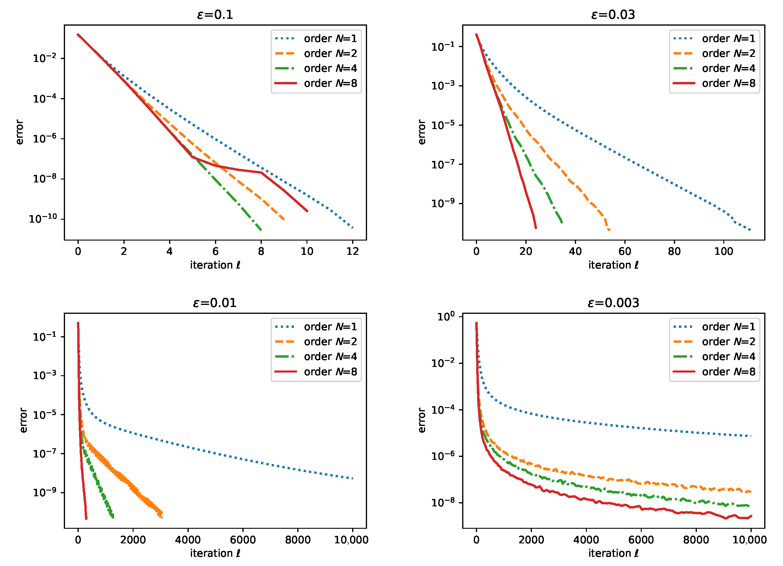
We first considered the relaxation parameter , in order to recover the original SK algorithm for . In Figure 1, we show the convergence results obtained with RNA orders on four regularized transport problems corresponding to entropic parameters . Figure 1 first illustrates that the convergence is improved with higher RNA orders N.
The acceleration is also greater for low values of the regularization parameter . This is an important behavior, as many iterations are required to have an accurate estimation of these challenging regularized transport problems. In the settings , a speedup of more than in terms of the iteration number was observed between RNA orders and (SK) to reach the same convergence threshold. We did not observe a significant improvement by considering higher RNA orders such as .
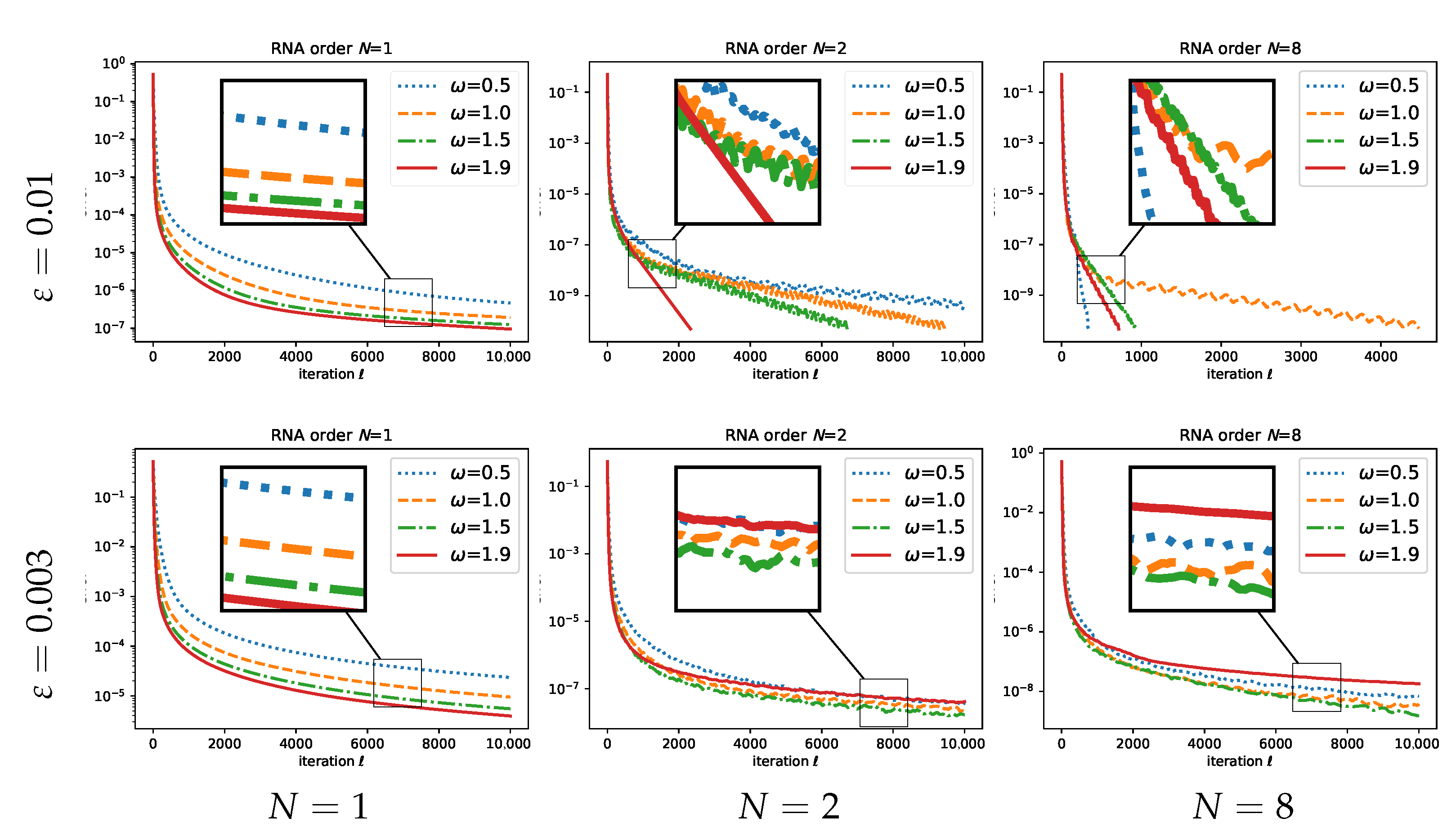
Next, we focus on the influence of the relaxation parameter onto the behavior of RNA schemes of orders . We restricted our analysis to the more challenging settings and . As illustrated in Figure 2, increasing systematically led to improvements in the case . For other RNA orders satisfying , we did not observe clear tendencies. Taking generally allowed accelerating the convergence.
To sum up, we recommend the use of the parametrization and when applying the RNA method to the SK algorithm.
We recall that the convergence of such approaches is not ensured. This last experiment nevertheless suggested that in the case , there is room to accelerate the original SK algorithm (), while keeping its global convergence guarantees, by looking at overrelaxed schemes with parameters .
3.3. Discussion
The nonlinear regularized acceleration algorithm involves relevant numerical accelerations without convergence guarantees. To build an algorithm that ensures the convergence of iterates, but also improves the numerical behavior of the SK algorithm, we now propose to follow a different approach using Lyapunov sequences, which is a classical tool to study optimization algorithms. The new scheme proposed here uses the specific form of the SK algorithm with the two variables and . It performs two successive overrelaxations (SOR) at each step, one for the update of and one for . The algorithm does not use any mixing scheme, but the simple structure allows defining a sequence, called a Lyapunov sequence, which decreases at each step. This Lyapunov approach allows ensuring the convergence of the algorithm for a suitable choice of the overrelaxation parameter.
The algorithm can be summarized as follows:
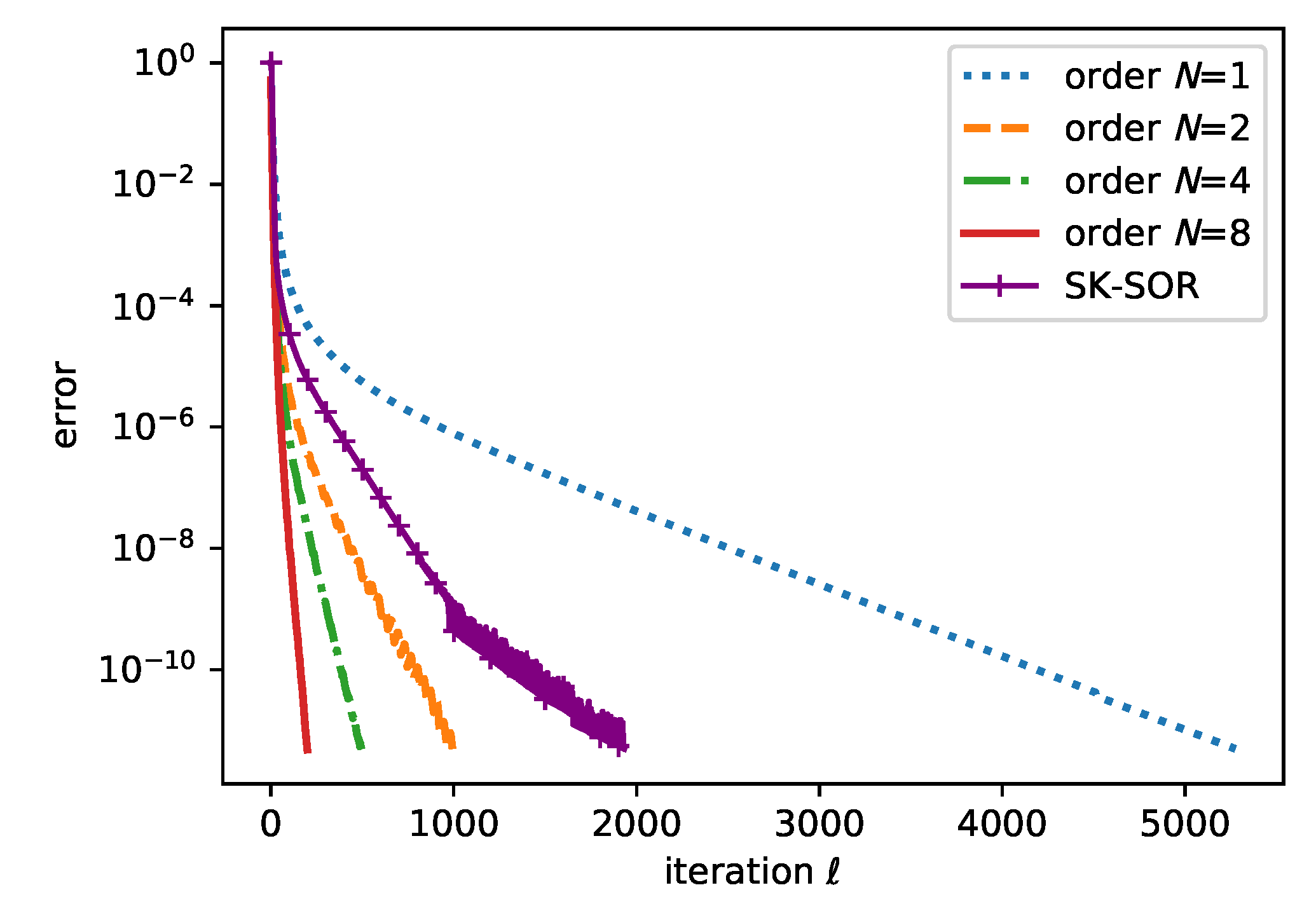
Our convergence analysis relied on an online adaptation of the overrelaxation parameter . As illustrated by Figure 3, in the case for , the proposed SK-SOR method was not as performant as high RNA orders with . It nevertheless gave an important improvement with respect to the original SK method, while being provably convergent.
4. Sinkhorn–Knopp with Successive Overrelaxation
In this section, we propose a globally convergent overrelaxed SK algorithm. Different from the RNA point of view of the previous section, our algorithm SK-SOR relies on successive overrelaxed (SOR) projections.
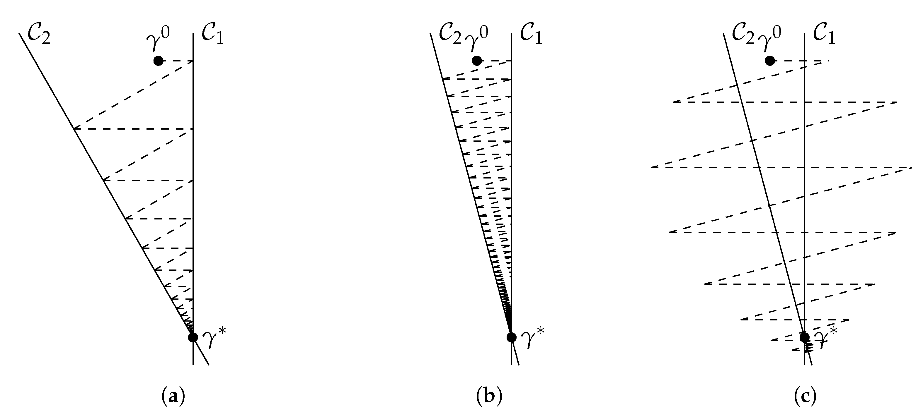
As illustrated in Figure 4a,b, the original SK algorithm (5) performs alternate Bregman projections (4) onto the affine sets and . In practice, the convergence may degrade when . The idea developed in this section is to perform overrelaxed projections in order to accelerate the process, as displayed in Figure 4c.
In what follows, we first define overrelaxed Bregman projections. We then propose a Lyapunov function that is used to show the global convergence of our proposed algorithm in Section 4.3. The local convergence rate is then discussed in Section 4.4.
4.1. Overrelaxed Projections
We recall that are operators realizing the Bregman projection of matrices onto the affine sets , , as defined in (4). For , we now define the -relaxed projection operator as:
where the logarithm is taken coordinate-wise. Note that is the identity, is the standard Bregman projection, and is an involution (in particular because is an affine subspace). In the following, we will consider overrelaxations corresponding to . A naive algorithm would then consist of iteratively applying for some choice of . While it often behaves well in practice, this algorithm may sometimes not converge even for reasonable values of . Our goal in this section is to make this algorithm robust and to guarantee its global convergence.
Remark 2.
Duality gives another point of view on the iterative overrelaxed Bregman projections: they indeed correspond to a successive overrelaxation (SOR) algorithm on the dual objective E given in (6). This is a procedure that, starting from , defines for ,
4.2. Lyapunov Function
Convergence of the successive overrelaxed projections is not guaranteed in general. In order to derive a robust algorithm with provable convergence, we introduced the Lyapunov function:
where denotes the solution of the regularized OT problem. We used this function to enforce the strict descent criterion as long as the process has not converged.
The choice of (23) as a Lyapunov function is of course related to the fact that Bregman projections are used throughout the algorithm. Further, we show (Lemma 1) that its decrease is simple to compute, and this descent criterion still allows enough freedom in the choice of the overrelaxation parameter.
Crucial properties of this Lyapunov function are gathered in the next lemma.
Lemma 1.
For any , the sublevel set is compact. Moreover, for any γ in , the decrease of the Lyapunov function after an overrelaxed projection can be computed as:
where
is a real function, applied coordinate-wise.
Proof.
The fact that the Kullback–Leibler divergence is jointly lower semicontinuous implies in particular that K is closed. Moreover, is bounded because F is the sum of nonnegative, coercive functions of each component of its argument .
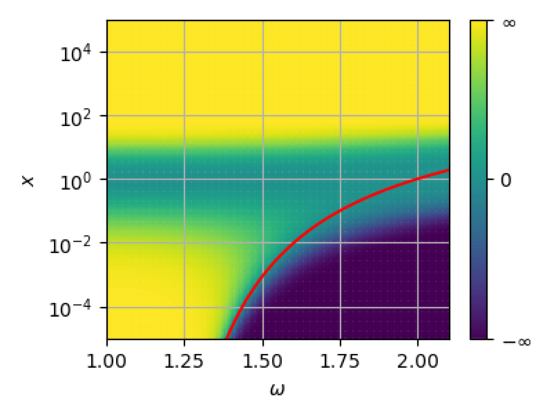
It follows from Lemma 1 that the decrease of F for an overrelaxed projection is very inexpensive to estimate, since its computational cost is linear with respect to the dimension of data . In Figure 5, we display the function . Notice that for the Sinkhorn–Knopp algorithm, which corresponds to , the function is always nonnegative. For other values , it is nonnegative for x close to one.
4.3. Proposed Algorithm
We first give a general convergence result that later serves as a basis to design an explicit algorithm.
Theorem 1.
Let and be two continuous functions of γ such that:
where the inequality is strict whenever . Consider the sequence defined by and:
Then, the sequence converges to .
Lemma 2.
Let us take in , and denote:
the set of matrices that are diagonally similar to . Then, the set contains exactly one element .
Proof.
We refer to [2] for a proof of this lemma. □
Proof of the Theorem.
First of all, notice that the operators apply a scaling to lines or columns of matrices. All are thus diagonally similar to :
By construction of the functions , the sequence of values of the Lyapunov function is non-increasing. Hence, is precompact. If is a cluster point of , let us define:
Then, by the continuity of the applications, . From the hypothesis made on and , it can be deduced that is in and is thus a fixed point of , while is in . Therefore, is in the intersection . By Lemma 2, , and the whole sequence converges to the solution. □
We can construct explicitly functions as needed in Theorem 1 using the following lemma.
Lemma 3.
Let . Then, for any , one has:
Moreover, equality occurs if and only if .
Proof.
Thanks to Lemma 1, one knows that:
The function that maps to is non-increasing since = Moreover, for , it is strictly decreasing. Thus, Inequality (27) is valid, with equality iff . □
We now argue that a good choice for the functions may be constructed as follows. Pick a target parameter , which will act as an upper bound for the overrelaxation parameter , and a small security distance . Define the functions and as:
where denotes the smallest coordinate of the vector w.
Proposition 1.
Proof.
Looking at Figure 5 can help understand this proof. Since the partial derivative of is nonzero for any , the implicit function theorem proves the continuity of . The function is such that every term in Relation (24) is non-negative. Therefore, by Lemma 3, using this parameter minus ensures the strong decrease (26) of the Lyapunov function. Constraining the parameter to preserves this property. □
This construction, which is often an excellent choice in practice, has several advantages:
- it allows choosing arbitrarily the parameter that will be used eventually when the algorithm is close to convergence (we motivate what are good choices for in Section 4.4);
- it is also an easy approach to having an adaptive method, as the approximation of has a negligible cost (it only requires solving a one-dimensional problem that depends on the smallest value of , which can be done in a few iterations of Newton’s method).
The resulting algorithm, which is proven to be convergent by Theorem 1, is written in pseudocode in Algorithm 2. The implementation in the log domain is also given in Algorithm 3. Both processes use the function defined implicitly in (29). The evaluation of is approximated in practice with a few iterations of Newton’s method on the function , which is decreasing, as can be seen in Figure 5. With the choice , one recovers exactly the original SK algorithm.
| Algorithm 2 Overrelaxed SK Algorithm (SK-SOR). |
| Require: , , Set , , , and while do , end while return |
| Algorithm 3 Overrelaxed SK Algorithm (SK-SOR) in the Log Domain. |
| Require: , , Set , , , and while do , , end while return |
4.4. Acceleration of the Local Convergence Rate
In order to justify the acceleration of convergence that is observed in practice, we now study the local convergence rate of the overrelaxed algorithm, which follows from the classical convergence analysis of the linear SOR method. Our result involves the second largest eigenvalue of the matrix:
where is the solution to the regularized OT problem (the largest eigenvalue is one, associated with the eigenvector ). We denote the second largest eigenvalue by ; it satisfies [36].
Proposition 2.
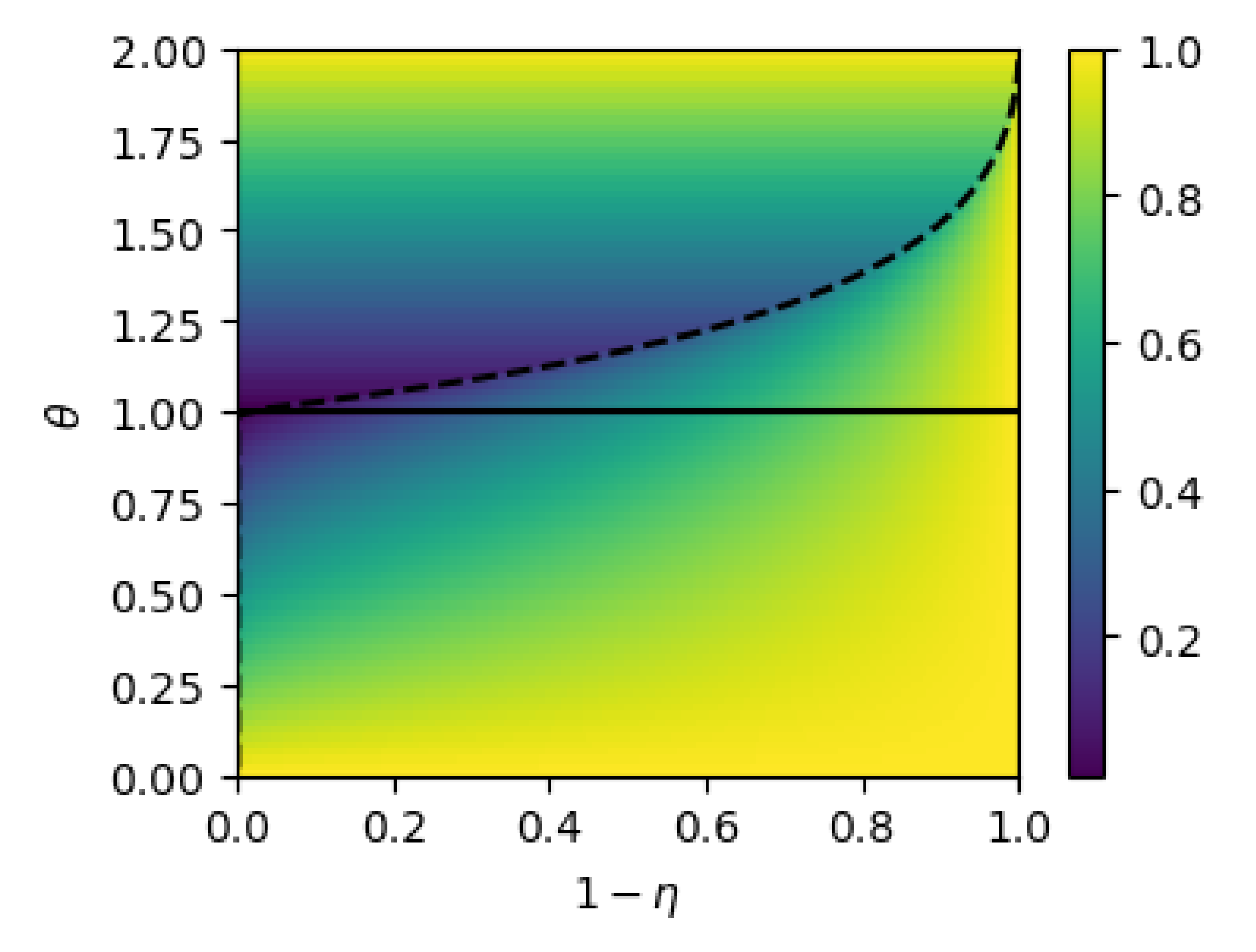
The SK algorithm converges locally at a linear rate . For the optimal choice of extrapolation parameter , algorithm SK-SOR converges locally linearly at a rate . The local convergence of SK-SOR is guaranteed for , and the linear rate is given in Figure 6 as a function of and θ.
Proof.
In this proof, we focus on the dual problem, and we recall the relationship between the iterates of the overrelaxed projection algorithm and the iterates of the SOR algorithm on the dual problem (21), initialized with . The dual problem (6) is invariant by translations of the form , , but is strictly convex up to this invariance. In order to deal with this invariance, consider the subspace S of pairs of dual variables that satisfy ; let be the orthogonal projection on S of kernel , and let be the unique dual maximizer in S.
Since one SK-SOR iteration is a smooth map, the local convergence properties of the SK-SOR algorithm are characterized by the local convergence of its linearization, which here corresponds to the SOR method applied to the maximization of the quadratic Taylor expansion of the dual objective E at . This defines an affine map whose spectral properties are well known [22,37] (see also [38] (Chapter 4) for the specific case of convex minimization and [39] for the non-strictly convex case). For the case , this is the matrix defined in Equation (31). The operator norm of is smaller than , so the operator converges at the linear rate towards zero (observe that by construction, and are co-diagonalizable and thus commute): for any , it holds . More generally, the convergence of is guaranteed for , with the linear rate:
This function is minimized with , which satisfies . The function f is plotted in Figure 6.
To switch from these dual convergence results to primal convergence results, we remark that implies , which in turn implies , so by invoking the partial strict concavity of E, we have . The converse implication is direct, so it holds . We conclude by noting the fact that converges at a linear rate, which implies the same rate on , thanks to the relationship between the iterates. □
Corollary 1.
The previous local convergence analysis applies to Algorithm 3 with Θ defined as in Equation (29), and the local convergence rate is given by the function of Equation (32) evaluated at the target extrapolation parameter .
Proof.
What we need to show is that eventually, one always has . This can be seen from the quadratic Taylor expansion , which shows that for any choice of , there is a neighborhood of one on which is nonnegative. □
5. Experimental Results
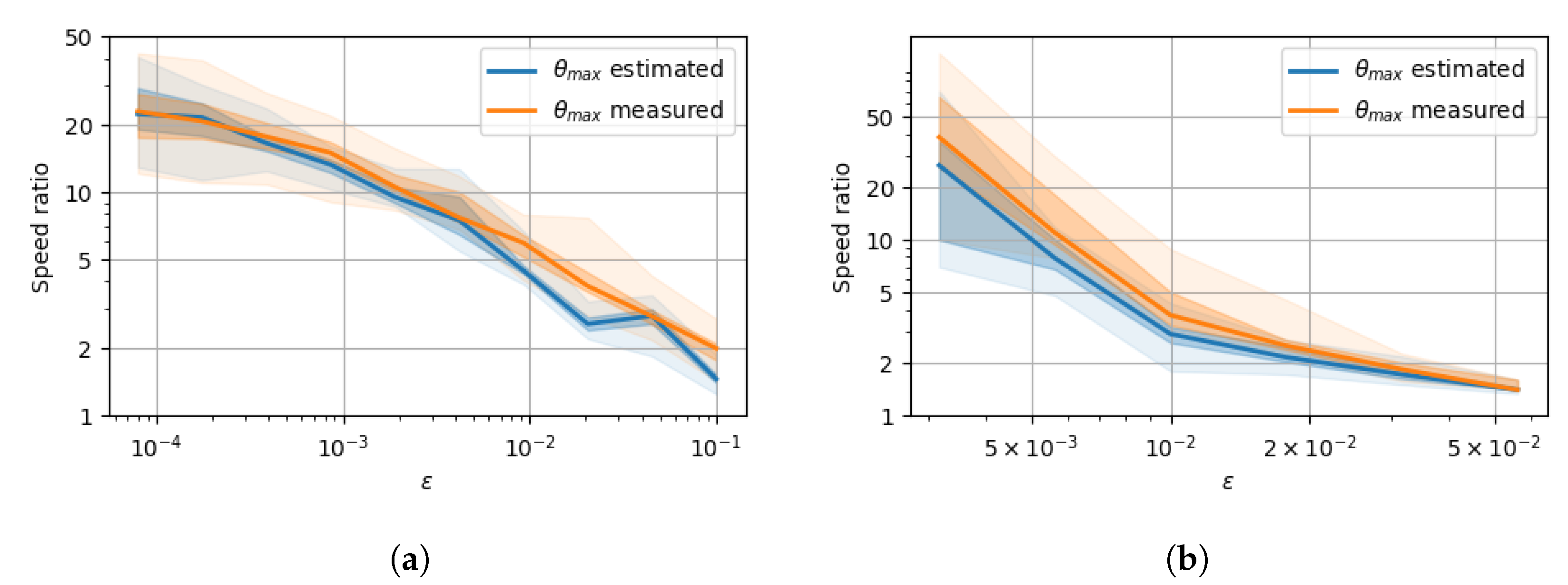
We compared Algorithm 2 to the SK algorithm on two very different optimal transport settings. In the setting of Figure 7a, we considered the domain discretized into 100 samples and the squared Euclidean transport cost on this domain. The marginals were densities made of the sum of a base plateau of height and another plateau of height and boundaries chosen uniformly in , subsequently normalized. In the setting of Figure 7b, the cost was a random matrix with entries uniform in , and the marginals were uniform.
Given an estimation of , the local convergence rate of the SK algorithm, we define as the optimal parameter as given in Proposition 2. For estimating , we followed two strategies. For strategy “estimated” (in blue on Figure 7), was measured by looking at the local convergence rate of the SK algorithm run on another random problem of the same setting and for the same value of . For strategy “measured” (in orange on Figure 7), the parameter was set using the local convergence rate of the SK algorithm run on the same problem. Of course, the latter was an unrealistic strategy, but it was interesting to see in our experiments that the “estimated” strategy performed almost as well as the “measured” one, as shown in Figure 7.
Figure 7 displays the ratio of the number of iterations required to reach a precision of on the dual variable for the SK algorithm and Algorithm 2. It is worth noting that the complexity per iteration of these algorithms is the same modulo negligible terms, so this ratio is also the runtime ratio (our algorithm can also be parallelized on GPUs just as the SK algorithm). In both experimental settings, for low values of the regularization parameter , the acceleration ratio was above 20 with Algorithm 2.
6. Conclusions and Perspectives
The SK algorithm is widely used to solve entropy-regularized OT. In this paper, we first showed that RNA methods are adapted to the numerical acceleration of the SK algorithm. Nevertheless, the global convergence of such approaches is not guaranteed.
Next, we demonstrated that the use of successive overrelaxed projections is a natural and simple idea to ensure and accelerate the convergence, while keeping many nice properties of the SK algorithm (first order, parallelizable, simple). We proposed an algorithm (SK-SOR) that adaptively chooses the overrelaxation parameter so as to guarantee global convergence. The acceleration of the convergence speed was numerically impressive, in particular in low regularization regimes. It was theoretically supported in the local regime by the standard analysis of SOR iterations. Nevertheless, the SK-SOR algorithm was not as performant as RNA, and no guarantee was given on the global computational complexity of either algorithm.
This idea of overrelaxation can be generalized to solve more general problems such as multi-marginal OT, barycenters, gradient flows, and unbalanced OT [38] (Chapter 4), but there is no systematic way to derive globally convergent algorithms. Our work is a step in the direction of building and understanding the properties of robust first-order algorithms for solving OT. More understanding is needed regarding SOR itself (global convergence speed, choice of ), as well as its relation to other acceleration methods [13,20].
Author Contributions
Methodology, A.T., L.C., C.D. and N.P.; Project administration, N.P.; Writing–original draft, A.T., L.C., C.D. and N.P. All authors have read and agreed to the published version of the manuscript.
Funding
This study was carried out with financial support from the French State, managed by the French National Research Agency (ANR) in the frame of the GOTMI project (ANR-16-CE33-0010-01).
Institutional Review Board Statement
Not applicable.
Informed Consent Statement
Not applicable.
Conflicts of Interest
The authors declare no conflict of interest.
References
- Rubner, Y.; Tomasi, C.; Guibas, L.J. The Earth Mover’s Distance As a Metric for Image Retrieval. Int. J. Comput. Vis. 2000, 40, 99–121. [Google Scholar] [CrossRef]
- Cuturi, M. Sinkhorn distances: Lightspeed computation of optimal transport. In Proceedings of the Advances in Neural Information Processing Systems 27, Lake Tahoe, NV, USA, 5–8 December 2013; pp. 2292–2300. [Google Scholar]
- Sinkhorn, R. A relationship between arbitrary positive matrices and doubly stochastic matrices. Ann. Math. Stat. 1964, 35, 876–879. [Google Scholar] [CrossRef]
- Seguy, V.; Cuturi, M. Principal geodesic analysis for probability measures under the optimal transport metric. In Proceedings of the Advances in Neural Information Processing Systems 29, Montreal, QC, Canada, 7–12 December 2015; pp. 3312–3320. [Google Scholar]
- Courty, N.; Flamary, R.; Tuia, D.; Rakotomamonjy, A. Optimal Transport for Domain Adaptation. arXiv 2015, arXiv:1507.00504. [Google Scholar] [CrossRef] [PubMed]
- Frogner, C.; Zhang, C.; Mobahi, H.; Araya-Polo, M.; Poggio, T. Learning with a Wasserstein Loss. arXiv 2015, arXiv:1506.05439. [Google Scholar]
- Montavon, G.; Müller, K.R.; Cuturi, M. Wasserstein Training of Restricted Boltzmann Machines. In Proceedings of the Advances in Neural Information Processing Systems 30, Barcelona, Spain, 29 November–10 December 2016; pp. 3718–3726.
- Rolet, A.; Cuturi, M.; Peyré, G. Fast Dictionary Learning with a Smoothed Wasserstein Loss. In Proceedings of the International Conference on Artificial Intelligence and Statistics (AISTATS), Cadiz, Spain, 9–11 May 2016; Volume 51, pp. 630–638. [Google Scholar]
- Schmitz, M.A.; Heitz, M.; Bonneel, N.; Ngole, F.; Coeurjolly, D.; Cuturi, M.; Peyré, G.; Starck, J.L. Wasserstein dictionary learning: Optimal transport-based unsupervised nonlinear dictionary learning. SIAM J. Imaging Sci. 2018, 11, 643–678. [Google Scholar] [CrossRef] [Green Version]
- Dessein, A.; Papadakis, N.; Rouas, J.L. Regularized optimal transport and the rot mover’s distance. J. Mach. Learn. Res. 2018, 19, 590–642. [Google Scholar]
- Rabin, J.; Papadakis, N. Non-convex Relaxation of Optimal Transport for Color Transfer Between Images. In Proceedings of the NIPS Workshop on Optimal Transport for Machine Learning (OTML’14), Quebec, QC, Canada, 13 December 2014. [Google Scholar]
- Chizat, L.; Peyré, G.; Schmitzer, B.; Vialard, F.X. Scaling Algorithms for Unbalanced Transport Problems. arXiv 2016, arXiv:1607.05816. [Google Scholar] [CrossRef]
- Altschuler, J.; Weed, J.; Rigollet, P. Near-linear time approximation algorithms for optimal transport via Sinkhorn iteration. In Proceedings of the Advances in Neural Information Processing Systems 31, Long Beach, CA, USA, 4–9 December 2017; pp. 1961–1971. [Google Scholar]
- Alaya, M.Z.; Berar, M.; Gasso, G.; Rakotomamonjy, A. Screening sinkhorn algorithm for regularized optimal transport. arXiv 2019, arXiv:1906.08540. [Google Scholar]
- Polyak, B. Some methods of speeding up the convergence of iteration methods. USSR Comput. Math. Math. Phys. 1964, 4, 1–17. [Google Scholar] [CrossRef]
- Ghadimi, E.; Feyzmahdavian, H.R.; Johansson, M. Global convergence of the Heavy-ball method for convex optimization. arXiv 2014, arXiv:1412.7457. [Google Scholar]
- Zavriev, S.K.; Kostyuk, F.V. Heavy-ball method in nonconvex optimization problems. Comput. Math. Model. 1993, 4, 336–341. [Google Scholar] [CrossRef]
- Ochs, P. Local Convergence of the Heavy-ball Method and iPiano for Non-convex Optimization. arXiv 2016, arXiv:1606.09070. [Google Scholar] [CrossRef] [Green Version]
- Anderson, D.G. Iterative procedures for nonlinear integral equations. J. ACM 1965, 12, 547–560. [Google Scholar] [CrossRef]
- Scieur, D.; d’Aspremont, A.; Bach, F. Regularized Nonlinear Acceleration. In Proceedings of the Advances in Neural Information Processing Systems 30, Barcelona, Spain, 5–10 December 2016; pp. 712–720. [Google Scholar]
- Scieur, D.; Oyallon, E.; d’Aspremont, A.; Bach, F. Online regularized nonlinear acceleration. arXiv 2018, arXiv:1805.09639. [Google Scholar]
- Young, D.M. Iterative Solution of Large Linear Systems; Elsevier: Amsterdam, The Netherlands, 2014. [Google Scholar]
- Peyré, G.; Chizat, L.; Vialard, F.X.; Solomon, J. Quantum Optimal Transport for Tensor Field Processing. arXiv 2016, arXiv:1612.08731. [Google Scholar]
- Dvurechensky, P.; Gasnikov, A.; Kroshnin, A. Computational optimal transport: Complexity by accelerated gradient descent is better than by Sinkhorn’s algorithm. In Proceedings of the International Conference on Machine Learning, Stockholm, Sweden, 10–15 July 2018; pp. 1367–1376. [Google Scholar]
- Lin, T.; Ho, N.; Jordan, M. On the efficiency of the Sinkhorn and Greenkhorn algorithms and their acceleration for optimal transport. arXiv 2019, arXiv:1906.01437. [Google Scholar]
- Lin, T.; Ho, N.; Jordan, M. On efficient optimal transport: An analysis of greedy and accelerated mirror descent algorithms. In Proceedings of the International Conference on Machine Learning, Long Beach, CA, USA, 10–15 June 2019; pp. 3982–3991. [Google Scholar]
- Thibault, A.; Chizat, L.; Dossal, C.; Papadakis, N. Overrelaxed sinkhorn-knopp algorithm for regularized optimal transport. arXiv 2017, arXiv:1711.01851. [Google Scholar]
- Lehmann, T.; von Renesse, M.K.; Sambale, A.; Uschmajew, A. A note on overrelaxation in the Sinkhorn algorithm. arXiv 2020, arXiv:2012.12562. [Google Scholar]
- Benamou, J.D.; Carlier, G.; Cuturi, M.; Nenna, L.; Peyré, G. Iterative Bregman projections for regularized transportation problems. SIAM J. Sci. Comput. 2015, 37, A1111–A1138. [Google Scholar] [CrossRef] [Green Version]
- Bregman, L.M. The relaxation method of finding the common point of convex sets and its application to the solution of problems in convex programming. USSR Comput. Math. Math. Phys. 1967, 7, 200–217. [Google Scholar] [CrossRef]
- Peyré, G.; Cuturi, M. Computational optimal transport. Found. Trends Mach. Learn. 2019, 11, 355–607. [Google Scholar] [CrossRef]
- Solomon, J.; de Goes, F.; Peyré, G.; Cuturi, M.; Butscher, A.; Nguyen, A.; Du, T.; Guibas, L. Convolutional Wasserstein Distances: Efficient Optimal Transportation on Geometric Domains. ACM Trans. Graph. 2015, 34, 1–11. [Google Scholar] [CrossRef]
- Richardson, L.F. IX. The approximate arithmetical solution by finite differences of physical problems involving differential equations, with an application to the stresses in a masonry dam. Philos. Trans. R. Soc. Lond. Ser. A Contain. Pap. A Math. Phys. Character 1911, 210, 307–357. [Google Scholar]
- Iutzeler, F.; Hendrickx, J.M. A generic online acceleration scheme for optimization algorithms via relaxation and inertia. Optim. Methods Softw. 2019, 34, 383–405. [Google Scholar] [CrossRef] [Green Version]
- Schmitzer, B. Stabilized sparse scaling algorithms for entropy regularized transport problems. arXiv 2016, arXiv:1610.06519. [Google Scholar] [CrossRef] [Green Version]
- Knight, P.A. The Sinkhorn–Knopp algorithm: Convergence and applications. SIAM J. Matrix Anal. Appl. 2008, 30, 261–275. [Google Scholar] [CrossRef] [Green Version]
- Ciarlet, P. Introduction à l’Analyse Numérique Matricielle et à l’Optimisation; Masson: Manchester, UK, 1982. [Google Scholar]
- Chizat, L. Unbalanced Optimal Transport: Models, Numerical Methods, Applications. Ph.D. Thesis, Université Paris Dauphine, Paris, France, 2017. [Google Scholar]
- Hadjidimos, A. On the optimization of the classical iterative schemes for the solution of complex singular linear systems. SIAM J. Algebr. Discret. Methods 1985, 6, 555–566. [Google Scholar] [CrossRef]
Figure 1.
Convergence of RNA schemes for a relaxation parameter and different orders . All approaches lead to similar convergence as the original SK algorithm (order , with blue dots) for high values of the entropic parameter such as . When facing more challenging regularized optimal transport problems, high-order RNA schemes () realize important accelerations. This behavior is highlighted in the bottom row for and . In these settings, with respect to SK, RNA of order (plain red curves) reduces by a factor 100 the number of iterations required to reach the same accuracy.

Figure 2.
Comparison of RNA schemes on an optimal transport problem regularized with the entropic parameters (top line) and (bottom line). The convergence of RNA scheme is illustrated for different relaxation parameters . Higher values of lead to larger improvements in the case (first column). When (as in the middle column for and the right column for ), it is not possible to conclude and to suggest a choice for the parameter with the obtained numerical results.

Figure 3.
Comparison between RNA schemes with and SK-SOR for a transport regularized with . The SK-SOR performance is in between the ones of RNA of orders and .
Figure 3.
Comparison between RNA schemes with and SK-SOR for a transport regularized with . The SK-SOR performance is in between the ones of RNA of orders and .

Figure 4.
The trajectory of given by the SK algorithm is illustrated for decreasing values of in (a,b). Overrelaxed projections (c) typically accelerate the convergence rate.
Figure 4.
The trajectory of given by the SK algorithm is illustrated for decreasing values of in (a,b). Overrelaxed projections (c) typically accelerate the convergence rate.

Figure 5.
Value of . The function is positive above the red line, negative below. For any relaxation parameter smaller than two, there exists a neighborhood of one on which is positive.
Figure 5.
Value of . The function is positive above the red line, negative below. For any relaxation parameter smaller than two, there exists a neighborhood of one on which is positive.

Figure 6.
Local linear rate of convergence of the SK-SOR algorithm as a function of , the local convergence rate of the SK algorithm, and the overrelaxation parameter. (Plain curve) The original rate is recovered for . (Dashed curve) Optimal overrelaxation parameter .
Figure 6.
Local linear rate of convergence of the SK-SOR algorithm as a function of , the local convergence rate of the SK algorithm, and the overrelaxation parameter. (Plain curve) The original rate is recovered for . (Dashed curve) Optimal overrelaxation parameter .

Figure 7.
Speed ratio between the SK algorithm and its accelerated SK-SOR version Algorithm 2 w.r.t. parameter . (a) Quadratic cost, random marginals; (b) Random cost, uniform marginals.
Figure 7.
Speed ratio between the SK algorithm and its accelerated SK-SOR version Algorithm 2 w.r.t. parameter . (a) Quadratic cost, random marginals; (b) Random cost, uniform marginals.

Publisher’s Note: MDPI stays neutral with regard to jurisdictional claims in published maps and institutional affiliations. |
© 2021 by the authors. Licensee MDPI, Basel, Switzerland. This article is an open access article distributed under the terms and conditions of the Creative Commons Attribution (CC BY) license (https://creativecommons.org/licenses/by/4.0/).
Share and Cite
MDPI and ACS Style
Thibault, A.; Chizat, L.; Dossal, C.; Papadakis, N. Overrelaxed Sinkhorn–Knopp Algorithm for Regularized Optimal Transport. Algorithms 2021, 14, 143. https://0-doi-org.brum.beds.ac.uk/10.3390/a14050143
AMA Style
Thibault A, Chizat L, Dossal C, Papadakis N. Overrelaxed Sinkhorn–Knopp Algorithm for Regularized Optimal Transport. Algorithms. 2021; 14(5):143. https://0-doi-org.brum.beds.ac.uk/10.3390/a14050143
Chicago/Turabian StyleThibault, Alexis, Lénaïc Chizat, Charles Dossal, and Nicolas Papadakis. 2021. "Overrelaxed Sinkhorn–Knopp Algorithm for Regularized Optimal Transport" Algorithms 14, no. 5: 143. https://0-doi-org.brum.beds.ac.uk/10.3390/a14050143
Note that from the first issue of 2016, this journal uses article numbers instead of page numbers. See further details here.