
Analysis and Prediction of Carsharing Demand Based on Data Mining Methods

School of Traffic and Transportation, Beijing Jiaotong University, Beijing 100044, China
*
Author to whom correspondence should be addressed.
Algorithms 2021, 14(6), 179; https://0-doi-org.brum.beds.ac.uk/10.3390/a14060179
Submission received: 12 May 2021
/
Revised: 31 May 2021
/
Accepted: 2 June 2021
/
Published: 5 June 2021
(This article belongs to the Special Issue Applications of Data Analytics, Simulation-Optimization, and Machine Learning in Services: From Sustainable Transportation and Supply Chains to Smart Cities, Health Care and Finance)
Abstract
:With the development of the sharing economy, carsharing is a major achievement in the current mode of transportation in sharing economies. Carsharing can effectively alleviate traffic congestion and reduce the travel cost of residents. However, due to the randomness of users’ travel demand, carsharing operators are faced with problems, such as imbalance in vehicle demand at stations. Therefore, scientific prediction of users’ travel demand is important to ensure the efficient operation of carsharing. The main purpose of this study is to use gradient boosting decision tree to predict the travel demand of station-based carsharing users. The case study is conducted in Lanzhou City, Gansu Province, China. To improve the accuracy, gradient boosting decision tree is designed to predict the demands of users at different stations at various times based on the actual operating data of carsharing. The prediction results are compared with results of the autoregressive integrated moving average. The conclusion shows that gradient boosting decision tree has higher prediction accuracy. This study can provide a reference value for user demand prediction in practical application.
1. Introduction
The basic concept of carsharing has existed for many years. A fleet of vehicles can be shared by several users, who can drive the vehicle when they need it, but they do not have to buy one themselves [1]. Compared with private vehicles, carsharing can offer the benefits of private vehicles without the costs and responsibilities of ownership [2]. It meets the individual demand of residents, such as leisure travel, business trips, and visiting friends. Carsharing can improve the utilization rate of resources and reduce the willingness of users to buy vehicles, thereby effectively alleviating the problems of environmental pollution, traffic congestion and excessive energy consumption. However, the development of the carsharing industry is immature, which faces many problems. Carsharing can be divided into station-based type and free-floating type. Unlike station-based carsharing, free-floating carsharing is not restricted by stations, and vehicles can be picked up and returned at will [3]. However, station-based carsharing also has its advantages. For example, operators can better manage vehicles and save human resources. Station-based carsharing is divided into one-way and round-way. In one-way carsharing, a general imbalance in vehicle demand exists at each station due to different pick-up and return stations, which is coupled with the uncertainty of users’ travel demand. Issues include the inability of users to return a vehicle because of insufficient parking space and the inability of users to pick up a vehicle at an available station, which will lead to a series of problems. The user experience is so bad that it affects the profitability of operators. Therefore, the travel demand characteristics of users need to be analyzed, thus enabling the demand of users to be predicted, which can not only reduce the imbalance of vehicles at the stations but also meet the demands of users.
Fully understanding the travel characteristics of carsharing users is the key to predicting user demand. For the analysis of user travel characteristics, scholars have conducted various studies. With regard to factors that affect users’ travel behavior, Kang et al. used transaction data provided by a carsharing operator in Seoul, South Korea, and performed multiple linear regression modeling with the number of carsharing transactions as a dependent variable and with three groups of independent variables: environment, demographic, and transportation variables [4]. Sioui et al. [5], Luca et al. [6], and Efthymiou at al. [7] conducted statistical analysis on users’ travel behavior through questionnaires and found that users’ travel behavior was influenced by many factors such as age, gender, and income. To study the influence of personal preference on the evolution of route flow, Tian Lijun et al. established a dynamic model of individual choice of routes [8]. The user’s personal preference was introduced to constantly update the model rules. The result showed that subjective and objective psychological factors will affect travelers’ choice of travel route.
In terms of user travel characteristics, Schmoeller et al. used German carsharing order data to analyze the spatiotemporal characteristics of user demand [9]. The date (day) of order distribution in the same space was clustered to explore the long-term factors and short-term factors that affect demand. Guo Ruixue et al. analyzed the dynamic changes of platform vehicle supply on different periods of working days and non-working days and identified the demand contradiction period [10]. The spatial travel characteristics of users were analyzed, and results showed that the users’ demand for network vehicle travel was obviously different between the morning peak and the evening peak of working days. Choi and Yoon analyzed the correlation between the supply of public transportation and the carsharing demand using the travel data of transportation cards and the trajectory data of carsharing in Seoul, South Korea [11]. Zohra et al. studied the purchase intention and product adjustment strategy of users with high price sensitivity by paying attention to users’ participation in consumption [12]. Hu et al. used the track number of taxis in Shenzhen to compare the temporal and spatial distribution characteristics of working days and non-working days. According to the different land use attributes, eight representative research areas (commercial areas, industrial areas, etc.) were selected to compare the changes of the demand for getting on and off a bus in different land use areas [13]. Hui et al. studied the track data of a carsharing company in Hangzhou, which operated in a round-way mode [14]. All travel chain modes are divided into five types for analysis. To intuitively understand the demand characteristics of carsharing travel users, this study also compares the carsharing travel chain with the private vehicle travel chain. Wang Xinxin et al. have studied the influence of consumer behavior through three psychological factors: price sensitivity, status preference, and evaluation scruples. The research shows that the three psychological factors not only affect users’ behavior to varying degrees but also have a close correlation [15]. According to the service data of free-floating carsharing in 23 cities in Europe and North America over a 14-month period, Giordano, Vassio, and Cagliero introduced the following characteristics in detail: fleet size, operating area, characteristics of vehicle bookings, and rentals. Results show that time rent distribution affects the usage of free-floating vehicles [16].
The travel demand of users is predicted after the travel characteristics of users are understood. Two main methods are used to study carsharing travel demand prediction: traditional mathematical modeling and data-driven modeling.
In traditional mathematical modeling, Zhou Xuemei et al. simplified the traditional model of four stages of traffic demand prediction on the basis of real-time road network travel data and historical-related data of residents’ travel [17]. With the use of the maximum information principle, the simplified model combined land use and road network flow to predict traffic demand. On the basis of the historical order data of Berlin, Müller and Bogenberger predicted the order quantity in each period of the next week in hours [18]. The ARIMA model and the Holt–Winters filtering model were used to predict the demand. The prediction effects of the two under different data quantities were also compared. Li Dongyue et al. established a diversion model based on dynamic demand to predict traffic demand in real time [19]. It fully considers the backward deviation evaluation index, real-time traffic flow density, real-time diversion ratio, road network evaluation index, and the backward result of the starting and ending matrix. Müller et al. used a negative binomial statistical model to fit the relationship between carsharing demand and other static factors in Berlin [20]. This study focused on two cities with a similar population size in Germany and compares the results with the actual booking results.
In terms of data-driven models, Alonso-Mora et al. proposed a data-driven optimization mathematical model that is suitable for a large number of passengers and journeys [21]. This model can dynamically generate the best route according to online demand and vehicle location. Wang Chunan et al. presented a demand prediction model that combines a distributed data processing framework with artificial neural network in a distributed computing environment. The prediction time is shortened by parallelizing the data of the artificial neural network in the distributed computing process [22]. Lin Yongjie et al. summarized the influencing factors of users’ short-term travel [23]. The correlation between various factors is explored. According to the results of correlation analysis, an artificial neural network model was established to predict the short-term travel demand of users. Li et al. proposed a dynamic user equilibrium model [24]. The model took free floating as an alternative transportation mode for daily activities. The path switching method is also proposed to solve the dynamic user equilibrium model based on fault tolerance. Le Vine et al. proposed a state response method to predict the usage of one-way carsharing. In this study, active behavior was used as the number of studies. The research tool is based on demand theory, and the activity type used in this study is shopping. This study only analyzes and quantifies the influence of the quantity related to shopping patterns. However, when the mode of transportation changes, shopping activities will also be affected [25]. Ampudia-Renuncio et al. evaluated the space of free-floating vehicles and obtained the time distribution of mainstream volume in the whole free-floating service area. Another value of this work lies in the spatial analysis of free-floating carsharing in Spain by using the collected data for the first time [26]. Daraio et al. proposed nonlinear machine learning models, which solve the problem of predicting the short-term availability of the free-floating carsharing service [27]. Cocca et al. studied the free-floating carsharing service demand prediction model and solved the demand prediction (i) over time and (ii) over space. Rich sociodemographic data are used to predict usage patterns, and the aim is to comprehensively compare the accuracy and ease of training of several machine learning algorithms and to evaluate the effectiveness of the current state-of-the-art methods to solve the prediction problem [28].
Previous studies on user travel characteristics have relatively simple considerations and do not analyze the travel characteristics of users comprehensively. In contrast, this study fully analyzes the travel characteristics of users. Demand prediction is constructed in combination with user travel characteristics. Most of the existing predicting studies lack instantaneity in carsharing demand prediction. Comprehensive modeling analyses from multiple dimensions, such as weather characteristics, are also lacking. Multi-dimensional influencing factors are fully considered in this study. Gradient boosting decision tree is established based on a large amount of actual operation data to predict the user’s demand in a short time. Therefore, this study is meaningful.
This study is structured as follows. First, the data are briefly introduced. According to the user’s order data, this study analyzes the user’s travel characteristics and the demand characteristics of station vehicles. On the basis of these characteristics, the stations and time are divided to establish GBDT. Then, GBDT is established based on actual operating data. A comparison of the results of GBDT with those of ARIMA shows that GBDT has higher prediction accuracy. The r analysis is conducted because GBDT considers not only its own historical value, but also the weather and demand situation of adjacent stations, among others. A series of discrete processing is performed on these characteristics and parameters in time to extract various characteristics as model inputs, thereby improving the prediction accuracy and applicability of the prediction results. Lastly, the conclusions of this study and suggestions for future research are presented.
2. Data and Data Preparation
2.1. Data Introduction
This study is based on operational data provided by a carsharing operating company in Gansu Province, China. The data used in this study are the data of 309,663 orders collected from May 2017 to September 2018. The main information includes order number, user number, order time, pick-up time, return time, pick-up station, and return station. An example of order data is shown in Table 1.
2.2. Statistic Description
User travel characteristics of demand are the key content of operator operation research. Understanding the travel characteristics and demand characteristics of carsharing users is the key to demand prediction.
2.2.1. User Travel Characteristics
- (1)
- Travel Characteristics During Holidays
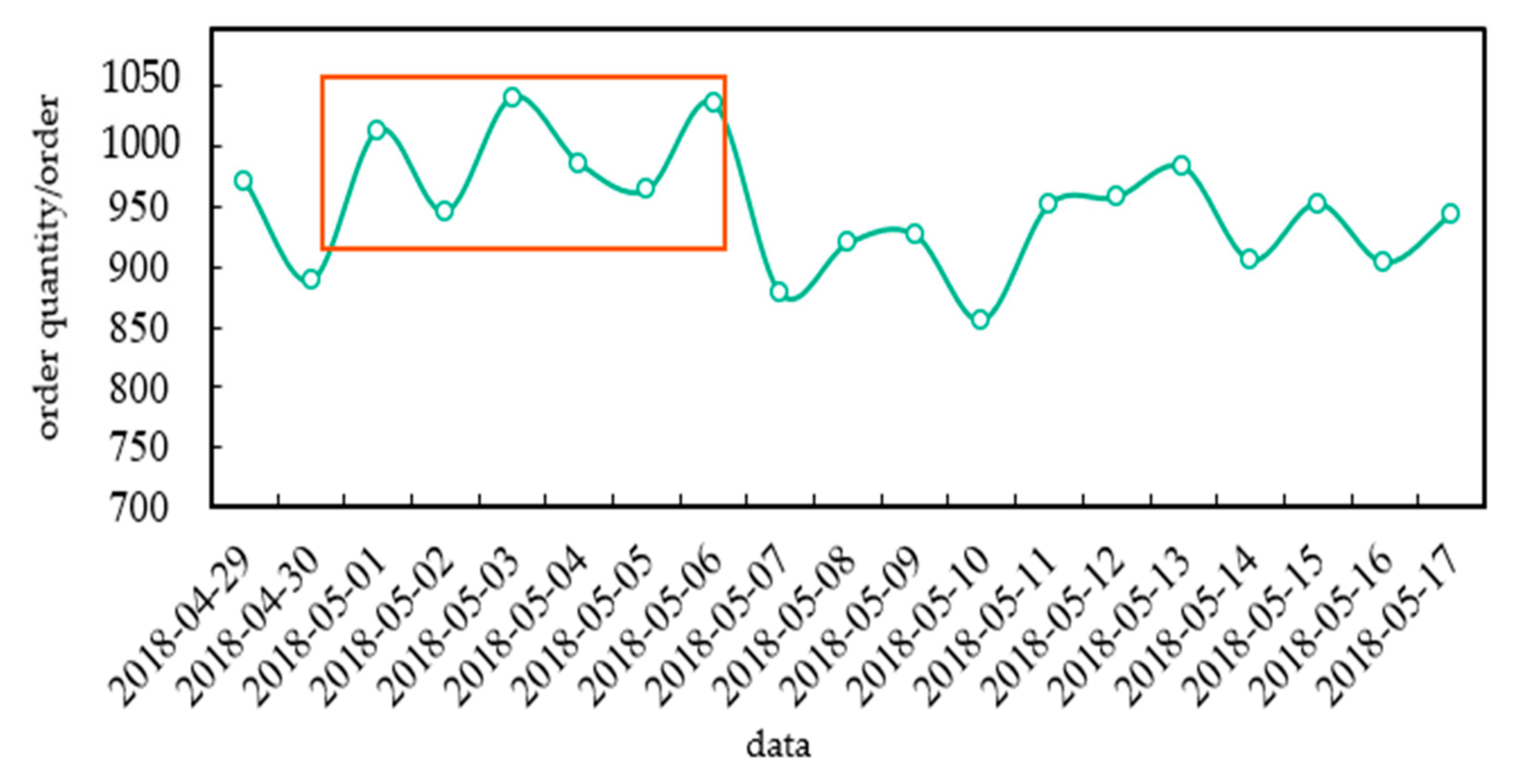
The order number of holidays is obviously higher than that of non-holidays. The daily order number from 29 April to 17 May 2018 is taken as the research object. Figure 1 shows that the demand during holidays from 1 May to 5 May is obviously higher than on other days, thus indicating that users have higher demand for carsharing during holidays.
- (2)
- Travel Characteristics on Weekdays and Weekends
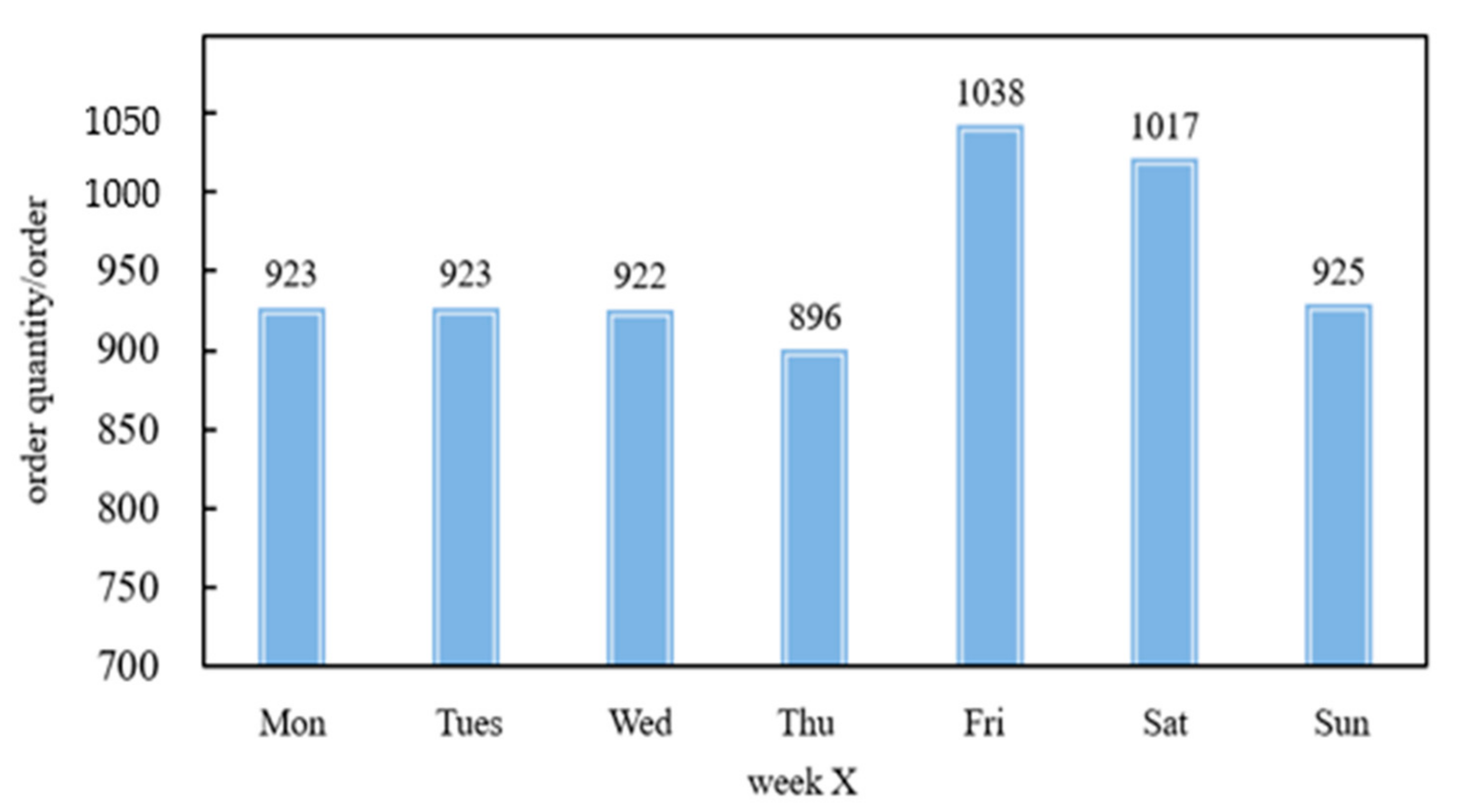
The study date is from 7 May to 17 June 2018. No holidays and large-scale event days took place during this time. Thus, the influence of special dates is excluded. The demand characteristics of users on weekdays and weekends are analyzed. As shown in Figure 2, the carsharing demand on Friday and Saturday is significantly higher than that on other days of the week, whereas the carsharing demand on Thursday is relatively lower.
2.2.2. Analysis of the Characteristics of Space–Time Demand
This study analyzes the demand characteristics of carsharing operators on the basis of user order data. It explores the evolution characteristics of the number of pick-up vehicles in different time and space scales. It also explores the distribution characteristic of imbalance demand in time and space.
- Characteristic of Time Demand
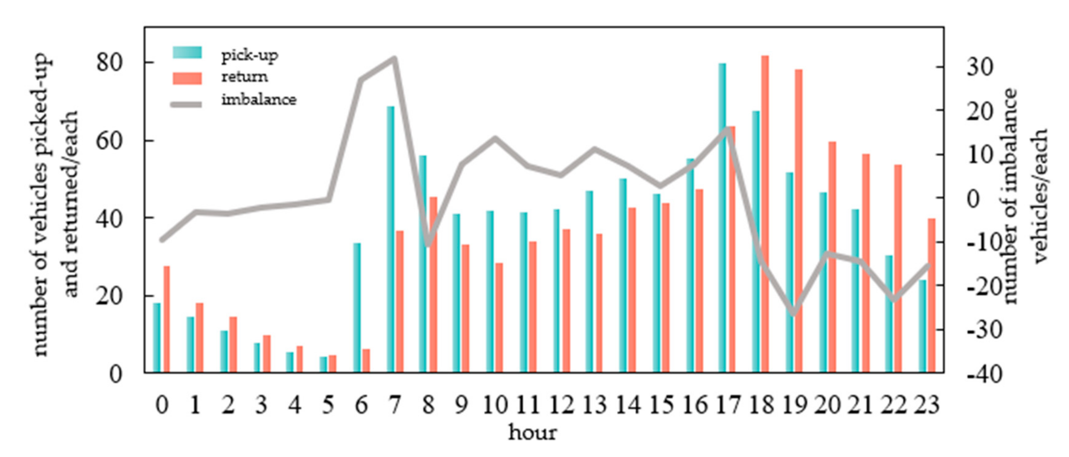
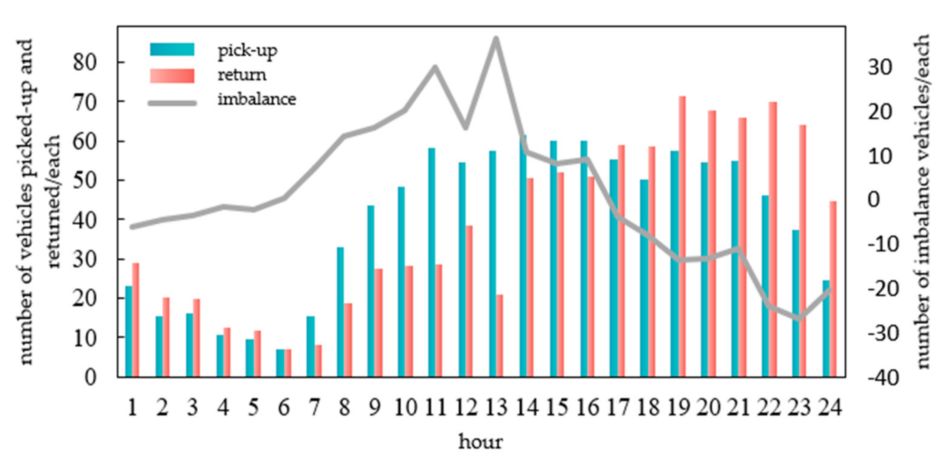
A carsharing operating system will have different demand at different times. In this study, one day is divided into 24 periods in hours. The number of picked-up and returned vehicles in each period of the weekday and weekend is counted. The number of imbalanced vehicles is also counted. As shown in Figure 3 and Figure 4, the number of picked-up vehicles is the number borrowed by users at each station, and the number of vehicles returned is the total number of vehicles returned by users at each station. The imbalance is the difference in the number of vehicles picked up and returned. On weekdays, the number of picked-up vehicles is higher in the morning and evening peak hours. The return time is concentrated after 17:00. The imbalance is serious in the morning peak of the working day. During weekends, no obvious peak of picked-up vehicles in the morning and evening occurs. The number of returned vehicles is concentrated in the afternoon and evening. During weekends, the imbalance of vehicles is serious between 11:00 and 14:00.
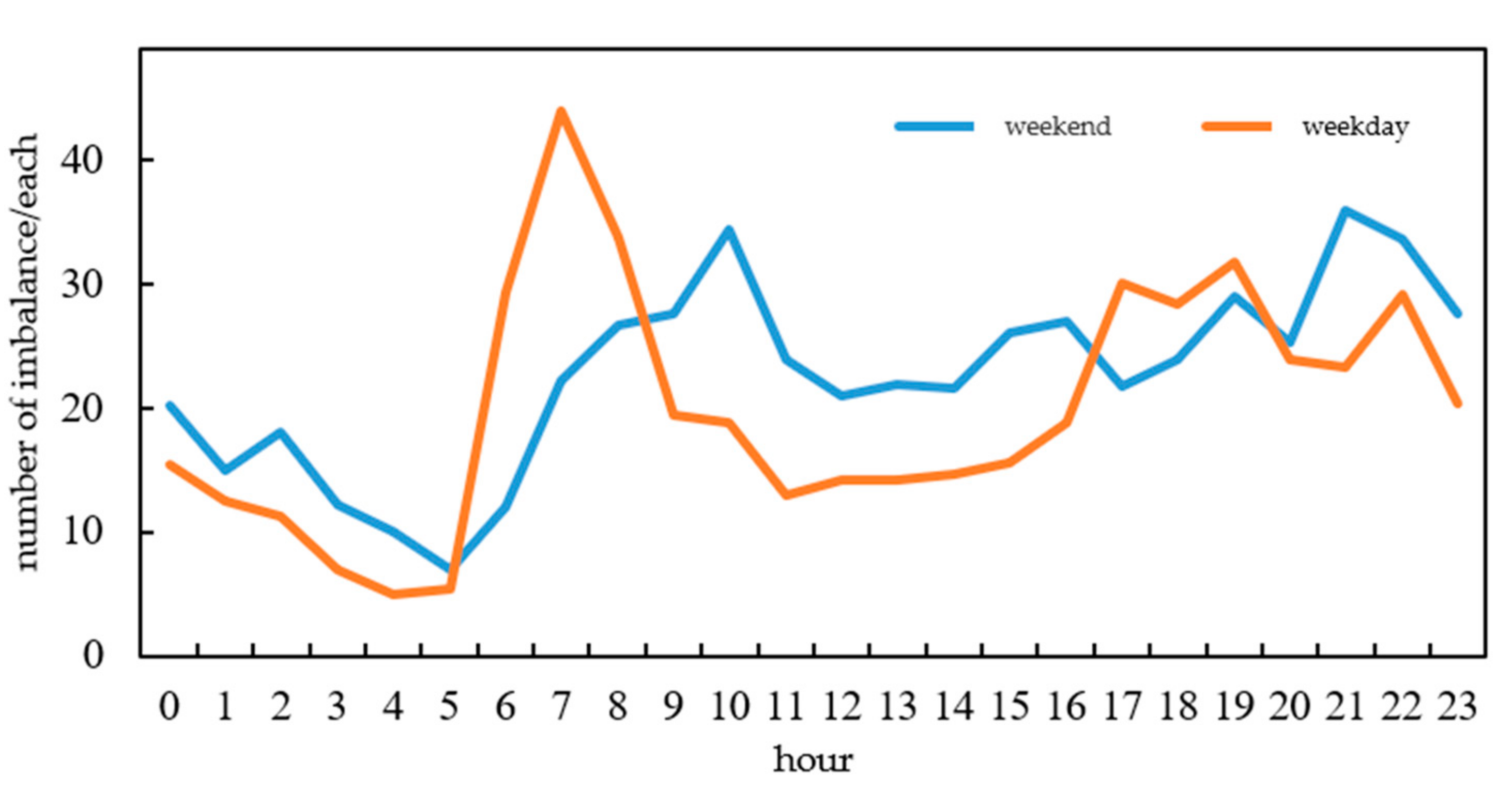
The imbalance in Figure 3 and Figure 4 is the overall imbalance after the system is superimposed. As a result of the relationship demand, each station will overlap positively and negatively to reduce the imbalance. This condition can not fully reflect the overall imbalance of the system. As shown in Figure 5, the absolute value of imbalance demand of each station is superimposed, thereby showing the accumulated imbalance demand of stations in different periods of weekdays and weekends. Moreover, an obvious peak imbalance is observed in the morning and evening of working days. On a weekday, the imbalance is relatively stable between 7:00 and 24:00. The peak trend is not obvious compared with that on weekdays.
- 2.
- Characteristic of Space Demand
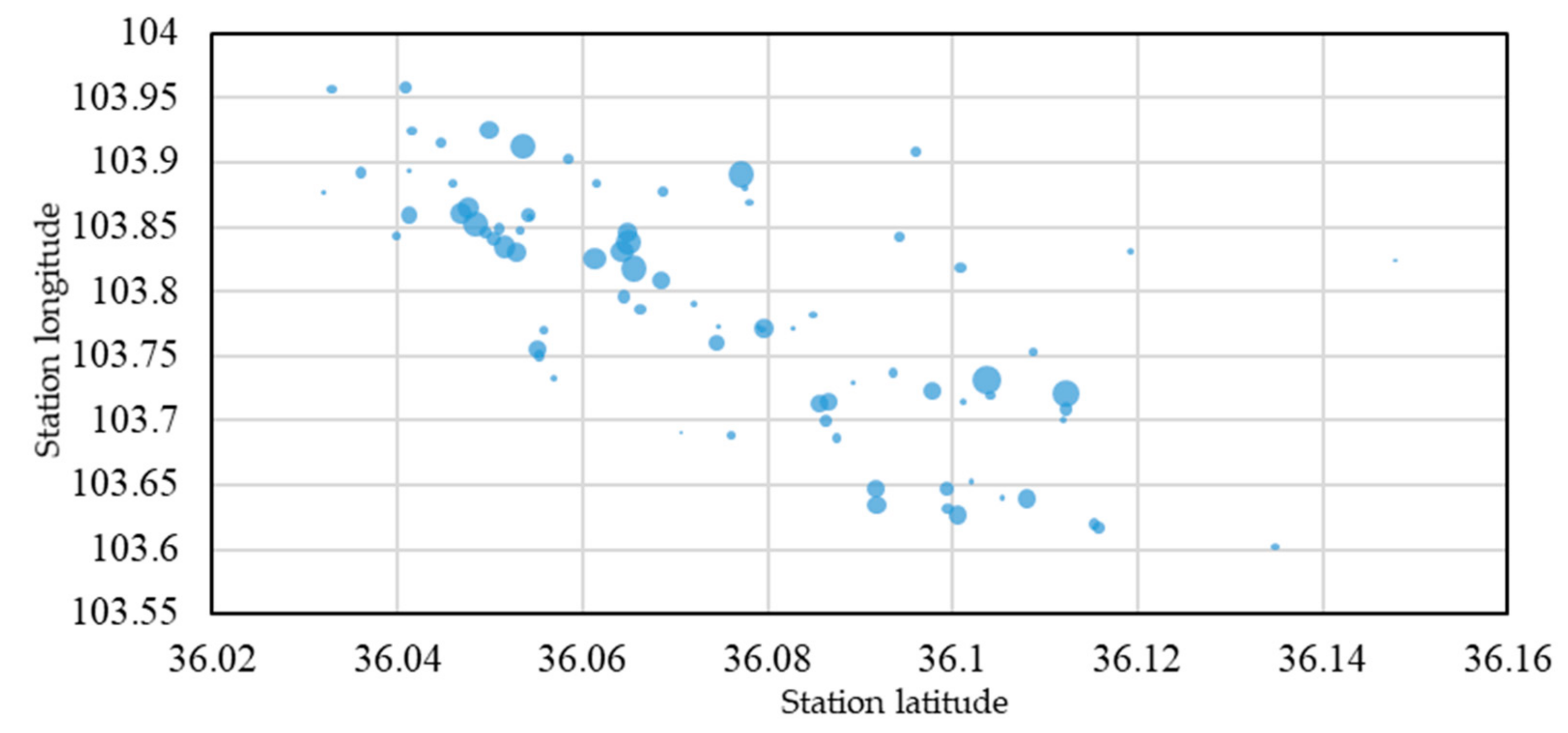
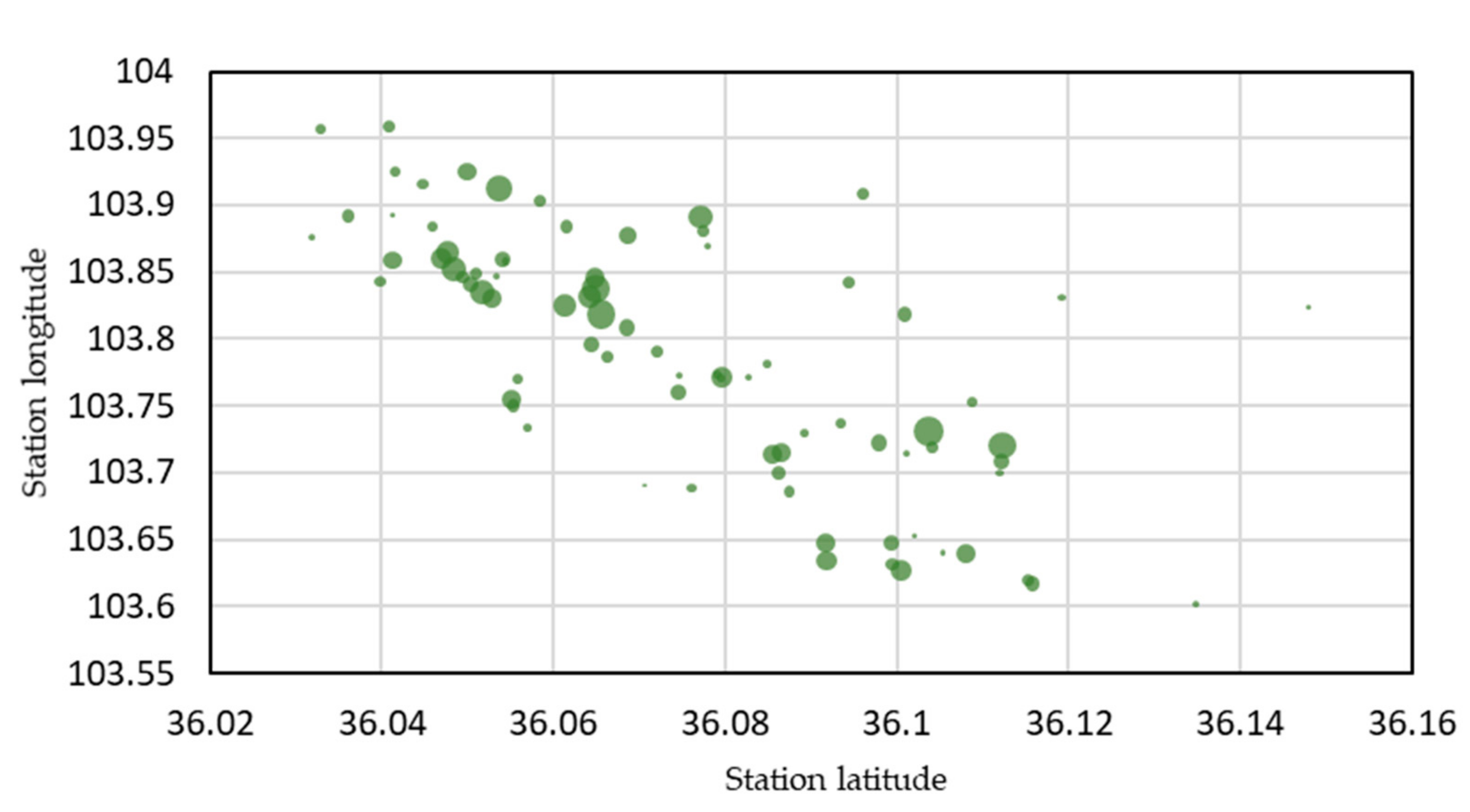
The number of vehicles picked up from the station is shown in Figure 6, while the number of vehicles returned to the station is shown in Figure 7. The bubble in the figure represents the station. Obvious differences are found in bubble distribution density. In places with dense stations, the bubbles are relatively large; that is, the number of vehicles picked up and returned is relatively large, which also reflects the rationality of the operator’s station layout from the side. However, where the stations are sparse, the bubbles are smaller; that is, fewer vehicles are picked up and returned.
2.3. Data Preparation
Referring to the results of user travel characteristics and station demand characteristics, this study divides the stations. In the following demand prediction, multiple stations in the same set are considered as one station for research. The reasons for the station division are as follows:
- (1)
- Users’ demand for picked-up vehicles is small due to the limited number of parking and vehicles in a single station. It is random and accidental; thus, accurately mining its change characteristic is impossible, and the demand cannot be predicted accurately.
- (2)
- The level of demand of adjacent stations is related to the degree of imbalance. Users located between several adjacent stations will adjust pick-up and return stations according to the real-time situation of the stations. Therefore, to make full use of the correlation between adjacent stations, adjacent stations can be classified into one class, considering the user’s selection behavior.
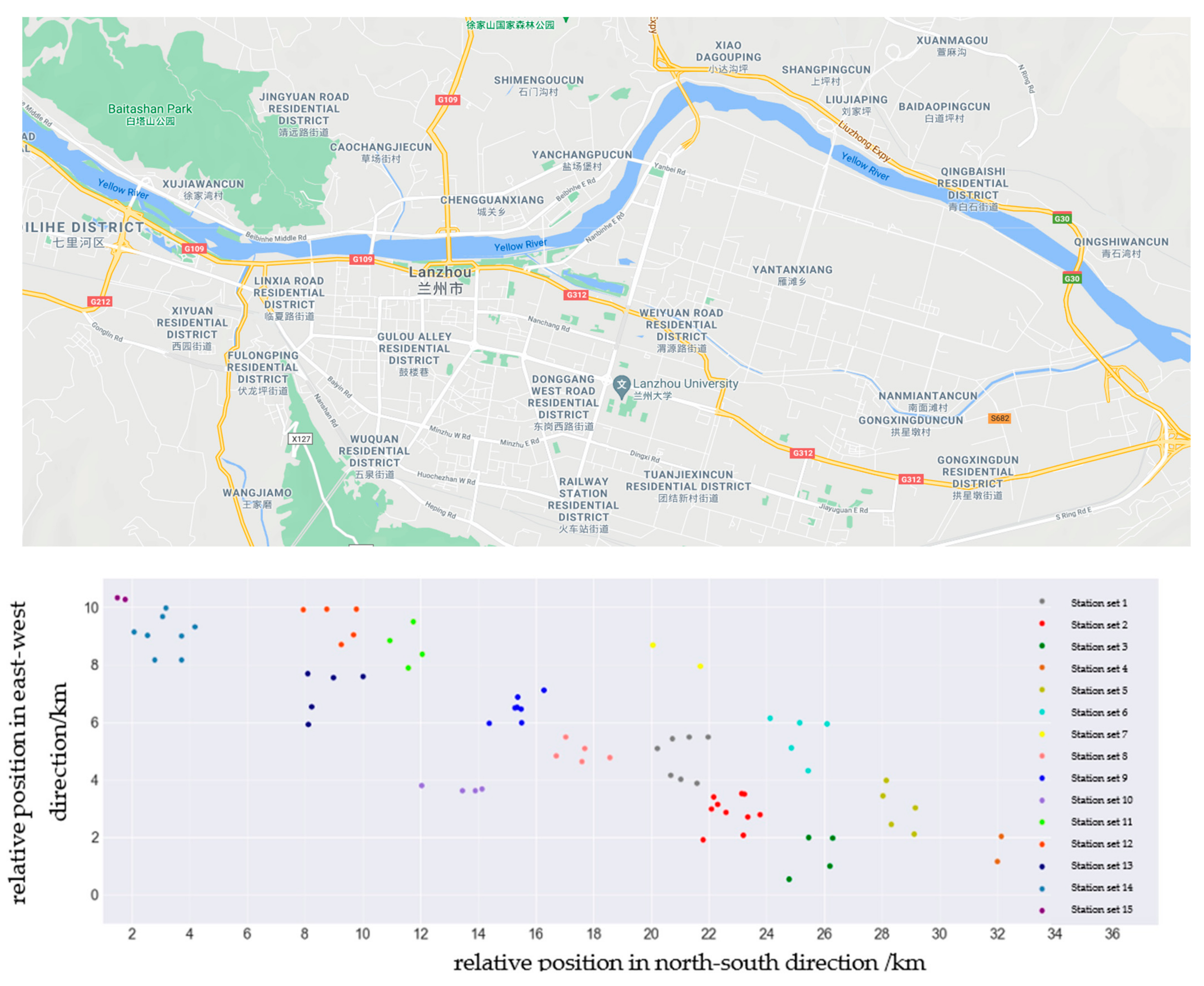
In this study, the location of each station on the map is determined according to latitude and longitude. The longitude and latitude of the station are transformed into Cartesian coordinates. The grid division method is adopted to divide the station into grids with a side length of 2 km. Proper manual adjustment is made to prevent the station from being too sparse. Stations where the average number of vehicles picked up in each period is less than 1 are discarded. Five obviously discrete stations are also discarded. The remaining 75 stations are divided into 15 station sets, as shown in Figure 8.
3. Prediction of Carsharing Demand Based on GBDT
This study is based on the operational data provided by a major carsharing operation company in Lanzhou, Gansu Province, China. GBDT is used for predicting demands. This study uses the results of station division in data preparation. It is based on the data of every three hours from 6:00 to 24:00 every day. The number of vehicles picked up by users in Area 1 is taken as the research object. The GBDT model is designed.
3.1. Test Set and Training Set
This experiment selects the four months of order data from 1 May to 31 August 2018 as the training set. The one-month data from 1 September to 29 September 2018 are used as the test set.
3.2. Characteristic Engineering
- (1)
- Characteristic Extraction of Weather Data
The model considers that a certain correlation exists between the users’ vehicle demand and the weather. Therefore, the characteristics of weather in each period are added. The characteristics of weather information are shown in Table 2.
- (2)
- Time Characteristics
Users’ demands will vary in different years, months, weeks, and periods. Therefore, time characteristics need to be added to improve the accuracy of the model, as shown in Table 3.
- (3)
- The historical number of vehicles picked up and returned at the target station, time information characteristics
User demand in a certain future period is closely related to the number of vehicles picked up and returned by users in a historical period. The following matrix is set to better construct characteristics:
Picked-up vehicles volume matrix:
Returned vehicles volume matrix:
where is the number of picked-up vehicles in the t-time period of day d; is the number of returned vehicles in the t-time period of day d.
According to the time characteristics of the number of picked-up and returned vehicles, the following characteristics can be constructed:
① On the basis of the short-term correlation of the sequence, the demand for a certain period of time in the future can be predicted based on the number of vehicles picked up and returned in the past six periods.
② On the basis of the daily similarity of the sequence, the demand for a certain period of time in the future can be predicted based on the number of picked up and returned vehicles in the same period in the past m days.
The vehicle demand in t period on d day is assumed to be predicted. The added characteristics are shown in Table 4.
- (4)
- Information Characteristics of Adjacent Station Collection
The regional center coordinates of station collections q are expressed as . The distance between each station set can be obtained by calling map data according to the coordinates of each station set. The coordinate calculation formula of station collection q is as follows:
is the station collection number;
is the i-th station of station ; and
is the cumulative number of picked-up vehicles at the i-th station of station .
The demand for the first t time period on the first d day is assumed to be predicted. The characteristics of the first three nearest stations are added, as shown in Table 5.
3.3. GBDT Algorithm Process
GBDT is a strong classifier formed by integrating many tree models and is a kind of boosting integration algorithm. The tree model in GBDT is the CART regression tree. The CART tree is divided into classification tree and regression tree, which includes three processes: characteristic selection, tree generation, and pruning. The CART regression tree is mainly used to learn and predict continuous values.
1. Building the CART regression tree
A binary tree is constructed recursively. Training data set D is continuously input into space and divided into two subregions. The optimal output value of each subregion is calculated.
Training data set D is input, and the CART regression tree is output.
If the generated regression tree is not pruned, then overfitting occurs easily. To ensure that the model is not overly complex, pruning operation should be carried out. The branches and leaves at the bottom of the CART regression tree are cut off, thus simplifying the regression decision tree, enhancing the generalization ability, and improving the accuracy of the model.
The CART generation algorithm uses the decision tree as input and optimal decision tree as output.
2. GBDT algorithm framework
- (1)
- Objective function and optimization
GBDT is a kind of supervised learning. The establishment of GBDT requires a large number of labeled datasets to support where is the size of the sample set, and ; is the label value. GBDT aims to give an estimation function for the real function . GBDT also aims to minimize the loss function to improve the prediction accuracy of the model. The estimation function is shown in Formula (5).
Formula (5) can be written in the form of a function that minimizes the expected loss as follows:
To make the goal of the problem more concrete, the search space is limited by parameter
. The formula is as follows:
Recursive numerical processes are usually used for optimization to solve the problem that the above functions may not have closed-form solutions. To improve the capability of the model, the value of the loss function in the negative gradient direction of the current model: is used to approximate the function residual and fit the regression tree.
GBDT is carried out to solve and predict by using the recursive method. At each stage of solving , starting from the weak classifier , a better model is obtained by adding estimator based on . As shown in Formula (8),
According to the principle of experience minimization,
On the problem of minimizing loss function, according to Formulas (9) and (10), the gradient descent method is used to update the model.
- (2)
- GBDT algorithm framework
Input: is the training set with labels; is the iterations; is the loss function; is the base learner; and GBDT is the output.
Step1: The model is initialized.
Step2: For k = 1 to M, the pseudo residual is calculated.
To obtain , the CART regression tree is used to fit the pseudo residuals. The weighting coefficient is calculated as follows:
Then, the model is updated.
Step 3: The final prediction model is obtained.
3.4. Importance of Parameters and Characteristics
- (1)
- Parameter Settings
The following parameters need to be set when the GBDT is constructed: L is the loss function; is the maximum depth of the tree; is the model iteration times; is the step size of each iteration.
When the parameters of the GBDT model are being adjusted, the iteration times and iteration steps should be determined first. Generally, the maximum depth of the tree should not exceed 20, so that the model is not too complicated or overfitted. Considering the accuracy of the model, the step size is set to 0.1. The root mean square error and mean absolute error are used as loss functions, and the parameters are optimized in the range of iteration times from 100 to 300 to select the iteration times with the highest accuracy of the model. Similarly, the step size and the depth of the tree are adjusted by grid search, and the parameter values that make the model work best are found.
- (2)
- Importance Calculation
To understand the contribution of each characteristic to the model prediction, the relative importance of each characteristic needs to be calculated. With the characteristic j taken as an example, the relative importance calculation formula is shown in (17).
where M is the iteration times;
is the importance of characteristic j in a single tree, as shown in Formula (18).
where
is the number of tree leaf nodes;
is the number of non-leaf nodes;
is the feature associated with node t;
is the average loss reduction value of node t after classification.
3.5. MAE and RMSE
RMSE and MAE are the evaluation indexes of machine learning. The formulas are shown in (19) and (20).
4. Results and Comparison
The following results are based on the actual operation data of a carsharing company in Lanzhou, Gansu Province, China. This experiment selects the four months of order data from 1 May to 31 August 2018 as the training set. The one-month data from 1 September to 29 September 2018 are used as the test set. It is based on the data of every three hours from 6:00 to 24:00 every day.
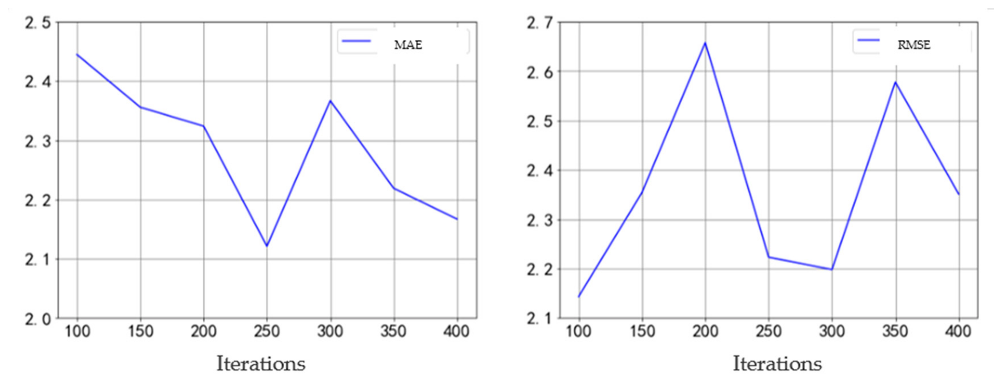
4.1. GDBT Prediction Result
The best iteration times are selected according to the parameter adjustment method. The variation trend of mean absolute error and root mean square error with iteration times is shown in Figure 9. With the change of iteration times, the average absolute error fluctuates from 2.1 to 2.5. When the number of iterations is 250, the average absolute error reaches the lowest. The root mean square error fluctuates from 2.1 to 2.7. When the number of iterations is 100, 250, and 300, the error is relatively small. Considering the average absolute error and root mean square error, the best number of iterations is 250.
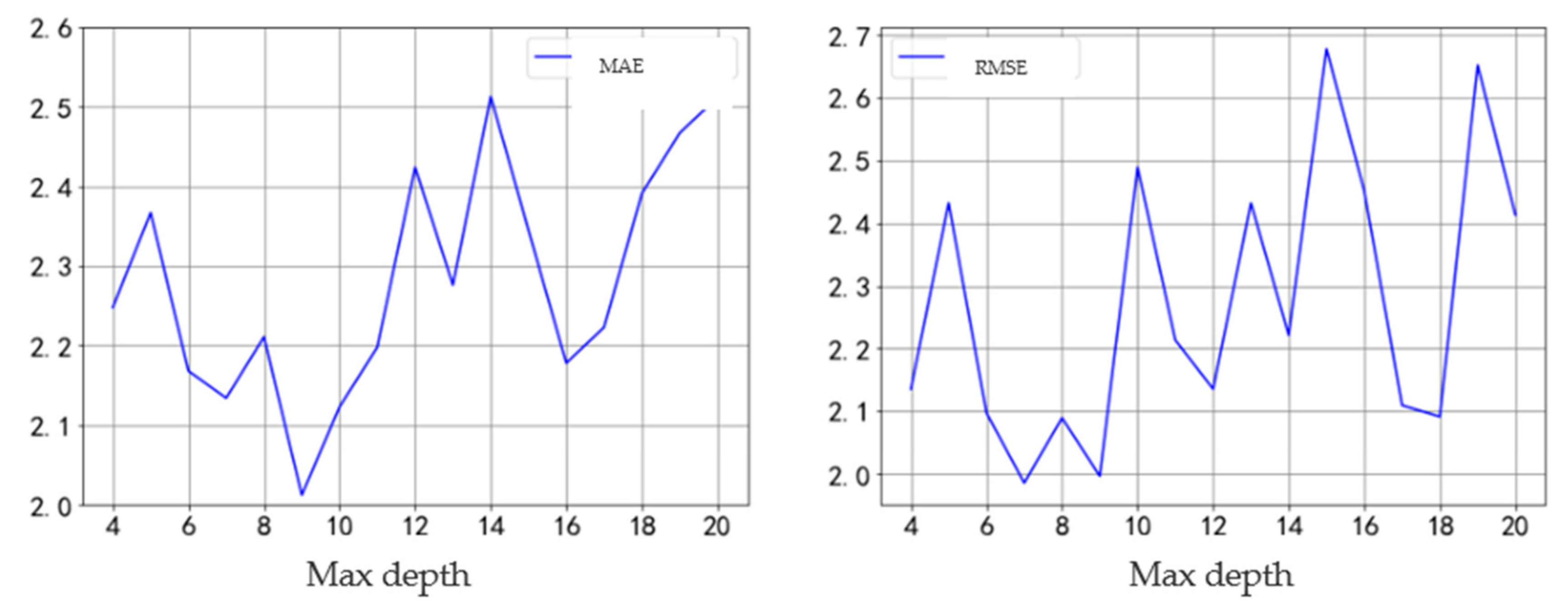
Next, the optimal max depth needs to be determined. The error statistical result is shown in Figure 10. The mean absolute error and root mean square error fluctuate with the increase in the maximum depth of the tree. When the depth is 9, both are small; that is, the optimal max depth is 9.
Similarly, parameters such as step size and loss function are searched in grid format. The optimal parameters of GBDT are obtained, as shown in Table 6.
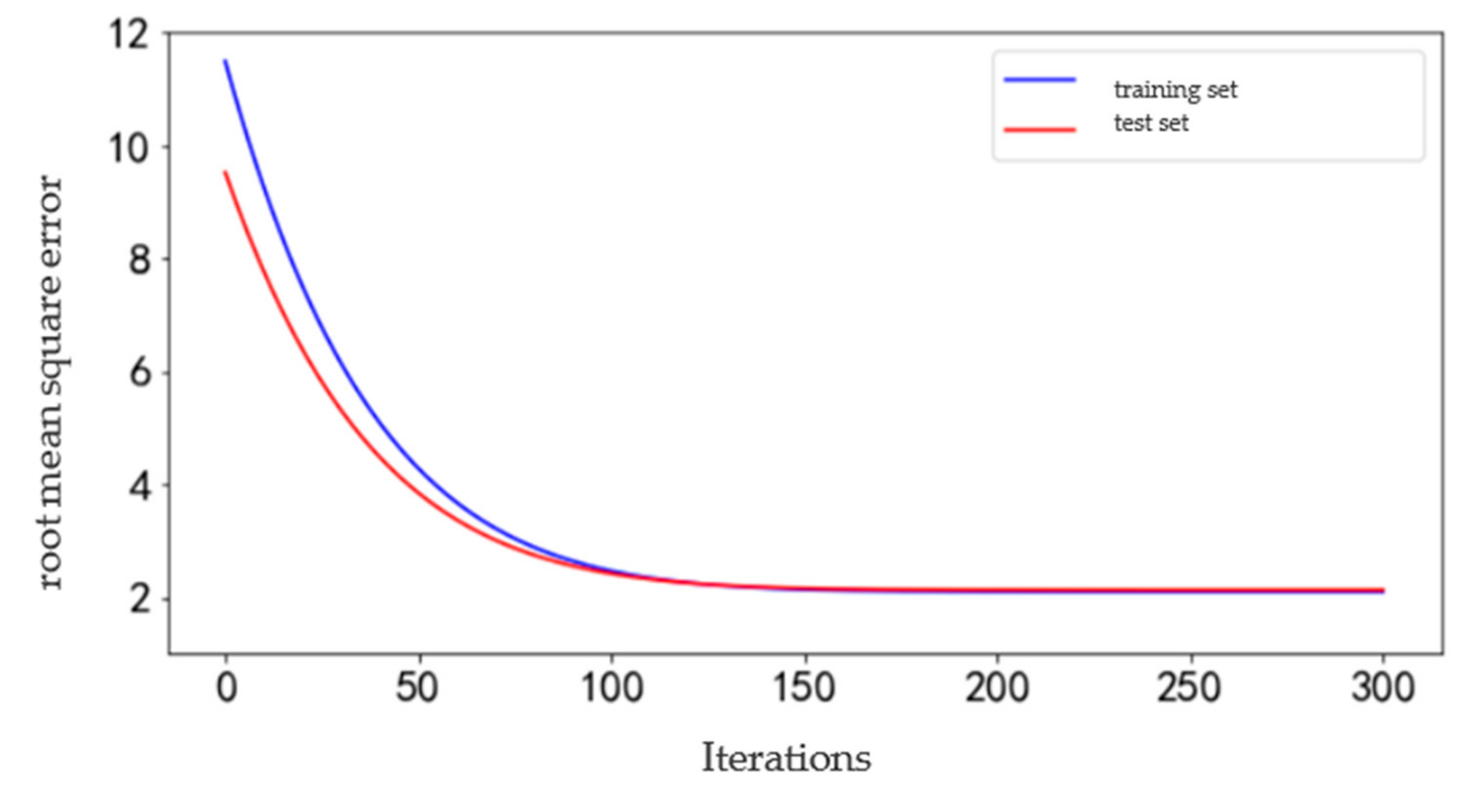
The GBDT is run according to the model’s optimal parameters in Table 6. The iterative results of the training set error and test set error are shown in Figure 11.
In accordance with Formula (6), the relative importance of some characteristics is derived. The GBDT, which plays a key role in predicting users’ demand, includes the time information, the number of vehicles picked up and returned in the previous period, the number of picked-up vehicles at the same time of the previous day, and so on.
4.2. Comparison
4.2.1. Analysis
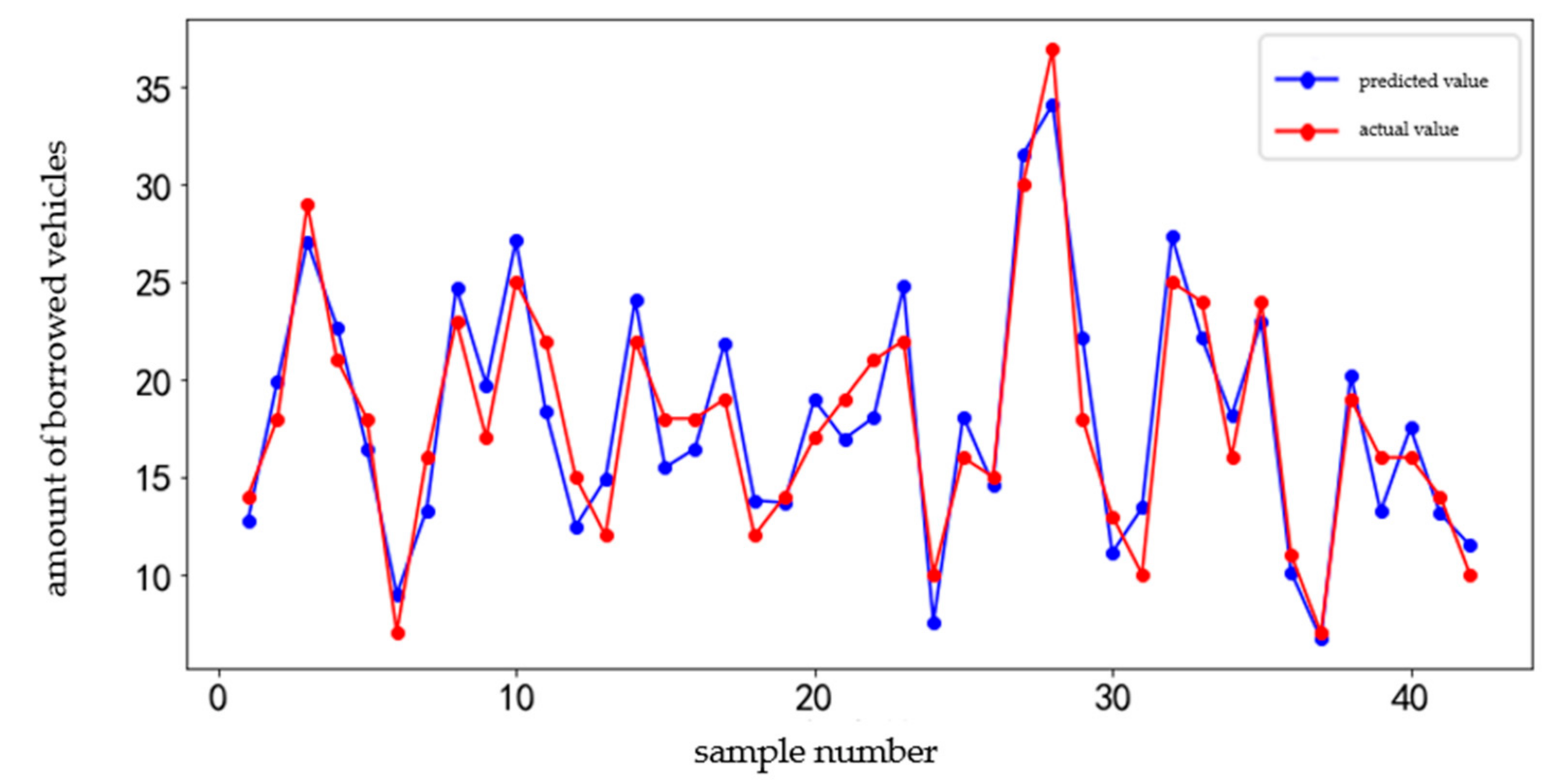
1. Analysis of GBDT
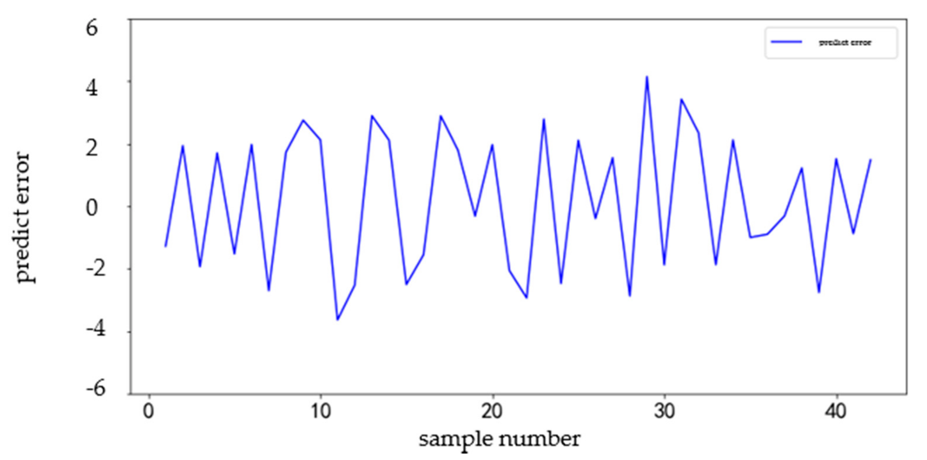
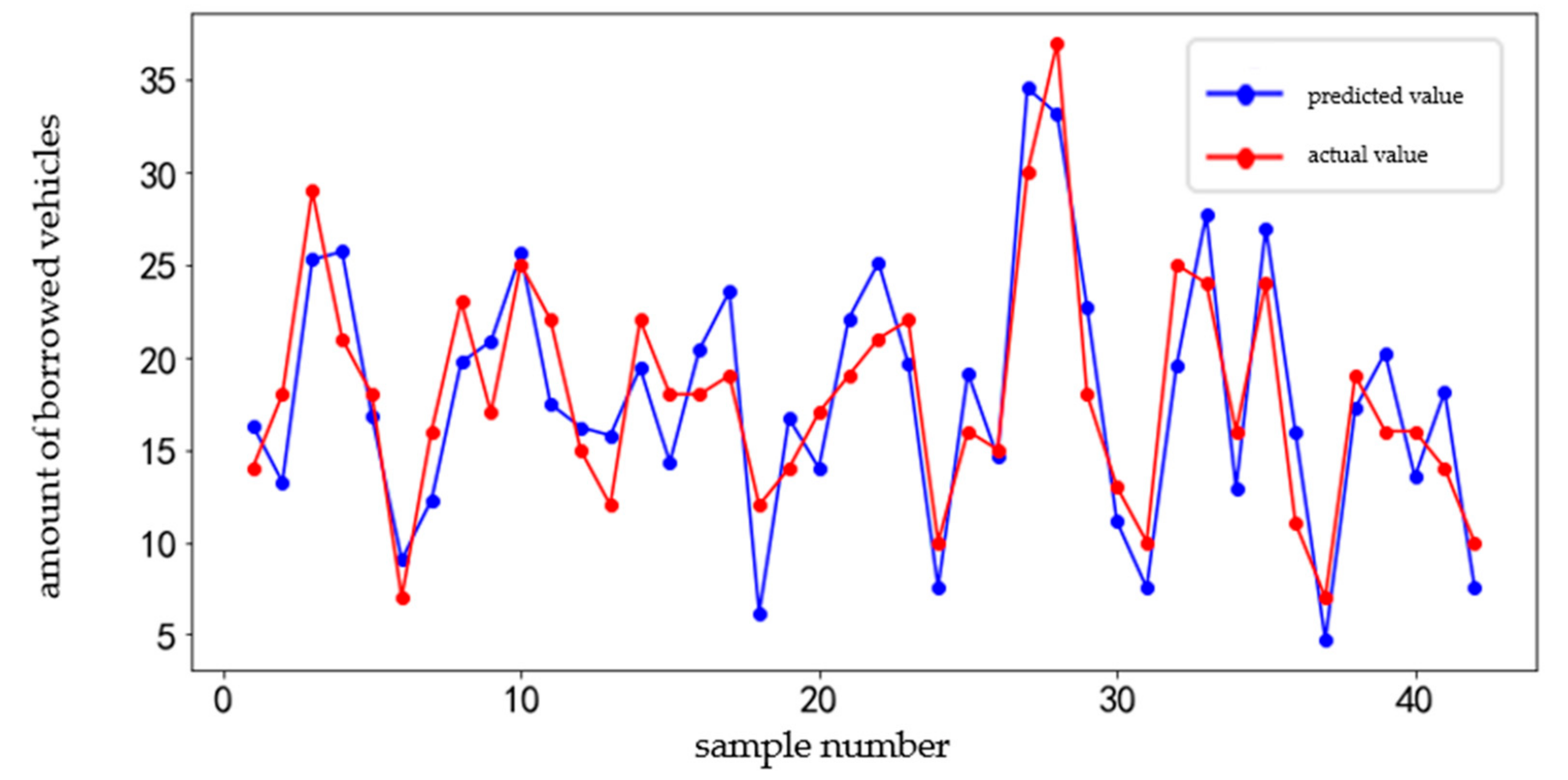
The seven-day data from 4 to 10 September 2018 of station set 1 are used as the test set to test the prediction accuracy of the model. The comparison between the predicted value and the actual value is shown in Figure 12. The prediction error is shown in Figure 13.
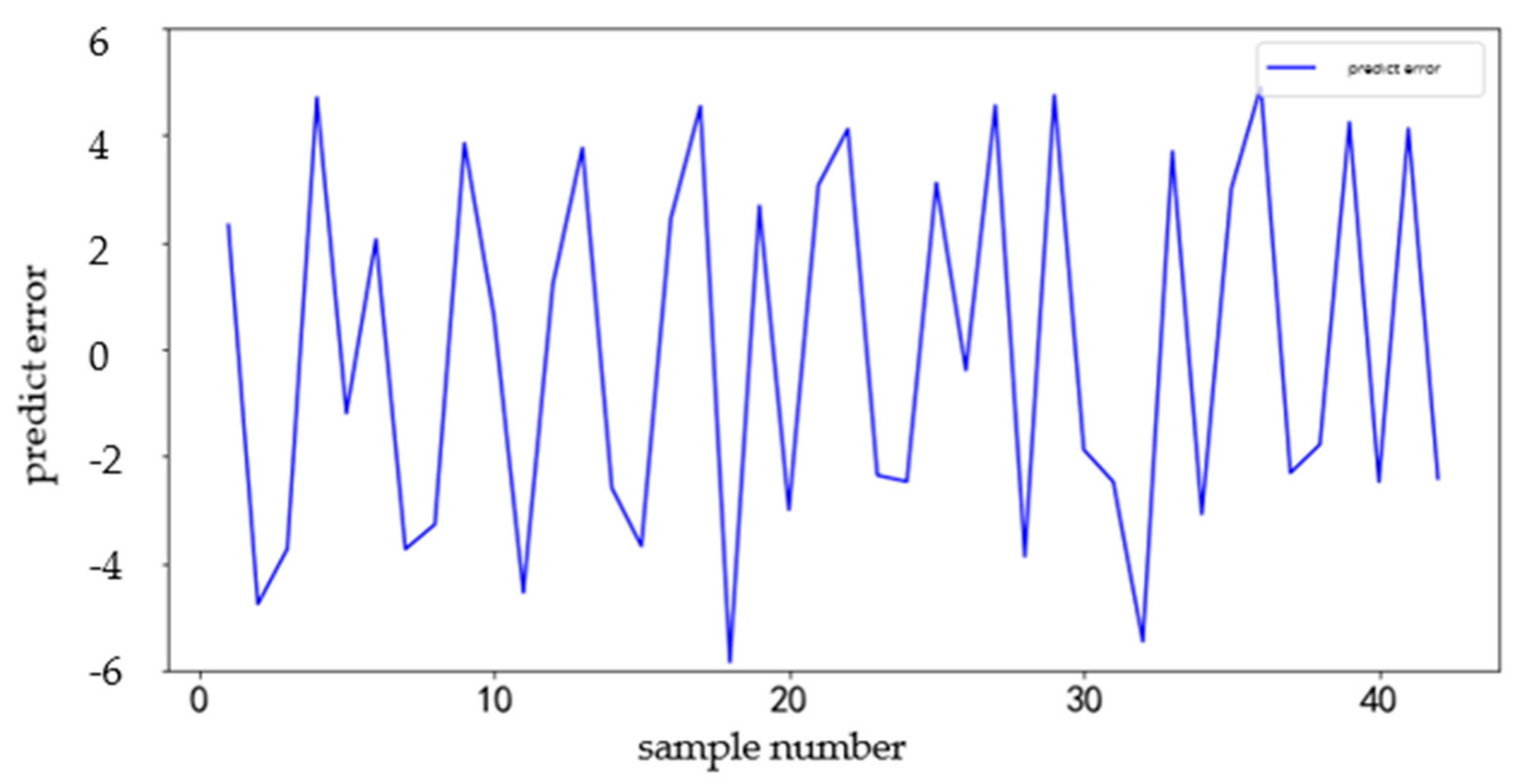
2. ARIMA analysis
4.2.2. Comparison
Other station sets are predicted in the same way as above. The demand level of each station set is different, which is why the predicted error value will also be different. The final prediction error analysis of GBDT and ARIMA is shown in Table 7.
Establishing ARIMA to predict users’ demands is feasible. However, the model still has the following problems:
- (1)
- The prediction error of user demand is still large, which will lead to unreliability in actual operation.
- (2)
- The ARIMA prediction model established in this study only highlights the role of time factor in prediction and does not consider the influence of external factors. When great changes take place in the outside world, great deviations will always occur.
RMSE and MAE are the evaluation indexes of machine learning. The formulas are shown in (19) and (20). According to the calculation formula, a small value corresponds to improved results. Then, when the value of MAE exceeds 2.5, the value is high, indicating that the prediction error is large. Therefore, the result is not of great value to operators.
The historical data of all stations from 4 to 10 September 2018 are used for verification to compare the advantages and disadvantages of the established ARIMA and GBDT. The comparison results of the prediction accuracy of the two models are shown in Table 8.
The comparison results in Table 8 indicate that the absolute value of each error item (maximum error, minimum error, average absolute error, and root mean square error) of GDBT is smaller than that of ARIMA. This result occurred because ARIMA only uses the influence of historical time series on the future. It does not consider the influence of other related factors. However, the GBDT not only considers its own historical value but also considers weather and the demand situation of adjacent stations, among other factors, thus improving the prediction effect of the model better. Thus, the GDBT model has higher prediction accuracy. So, it has a better reference value for user demand prediction in practical application.
5. Conclusions
On the basis of actual operation data, this study analyzes the travel characteristics and demand characteristics of users in depth. GBDT is proposed to predict the travel demand of users. Compared with ARIMA, GDBT has higher prediction accuracy. Unlike [27], both ARIMA and GBDT use a nonlinear algorithm. Ref. [27] proposed an overall framework for analyzing historical free-floating carsharing service usage data and predicting short-term vehicle availability. In addition, the proposed framework allows us to analyze spatial and temporal context conditions. However, its considerations are not very comprehensive. Compared with [28], [28] comprehensively compares various machine learning methods. Moreover, random regression forest is a more useful method. Various influencing factors are considered in this study, such as historical demand status of adjacent stations, weather conditions, and so on. The parameters of these factors are discretized in time. Dozens of dimensional characteristics are extracted as model inputs, and the prediction accuracy is improved. However, this study still has some shortcoming. The data of this study are taken from carsharing operators in Lanzhou, Gansu Province, China. However, different cities and operators have different characteristics. Few factors are considered in this study. Price, travel reasons, and other factors will also affect users’ willingness to use carsharing. Whether a user has coupons or not will also affect their choice. In the future, we hope to obtain more data and improve the prediction accuracy.
Author Contributions
Conceptualization and methodology, C.W. and J.B.; formal analysis, J.B.; validation, J.B.; writing—original draft, C.W.; wring—review and editing, Q.S. and J.B.; supervision, Z.Y. All authors have read and agreed to the published version of the manuscript.
Funding
This work is partially supported by the National Natural Science Foundation of China under Grant [No. 71961137008] and National Natural Science Foundation of China [No. 71621001].
Informed Consent Statement
Informed consent was obtained from all subjects involved in the study.
Data Availability Statement
The data is not available due to business data privacy.
Conflicts of Interest
The authors declare no conflict of interest.
References
- Ciari, F.; Bock, B.; Balmer, M. Modeling station-based and free-floating carsharing demand: Test case study for Berlin. Transp. Res. Rec. 2014, 2416, 37–47. [Google Scholar] [CrossRef]
- Shaheen, S.A.; Cohen, A.P. Growth in worldwide carsharing: An international comparison. Transp. Res. Rec. 2007, 1992, 81–89. [Google Scholar] [CrossRef] [Green Version]
- Ampudia-Renuncio, M.; Guirao, B.; Molina-Sanchez, R.; Bragança, L. Electric Free-Floating Carsharing for Sustainable Cities: Characterization of Frequent Trip Profiles Using Acquired Rental Data. Sustainability 2020, 12, 1248. [Google Scholar] [CrossRef] [Green Version]
- Kang, J.; Hwang, K.; Park, S. Finding factors that influence carsharing usage: Case study in seoul. Sustainability 2016, 8, 709. [Google Scholar] [CrossRef] [Green Version]
- Sioui, L.; Morency, C.; Trépanier, M. How carsharing affects the travel behavior of households: A case study of Montréal, Canada. Int. J. Sustain. Transp. 2013, 7, 52–69. [Google Scholar] [CrossRef]
- De Luca, S.; Di Pace, R. Modelling users’ behaviour in inter-urban carsharing program: A stated preference approach. Transp. Res. Part A Policy Pract. 2015, 71, 59–76. [Google Scholar] [CrossRef]
- Efthymiou, D.; Antoniou, C. Modeling the propensity to join carsharing using hybrid choice models and mixed survey data. Transp. Policy 2016, 51, 143–149. [Google Scholar] [CrossRef]
- Tian, L.; Jiang, X.; Liu, T.; Zhao, Y. Study on Daily Travel Behavior Considering Path Preference Based on Dogit Model. Transp. Syst. Eng. Inf. 2016, 16, 228–235. [Google Scholar]
- Schmoeller, S.; Weikl, S.; Mueller, J.; Bogenberger, K. Empirical analysis of free-floating carsharing usage: The Munich and Berlin case. Transp. Res. 2015, 56, 34–51. [Google Scholar] [CrossRef]
- Guo, R. Short-Term Predict of Online Car-Hailing Travel Demand Based on BP Neural Network; Beijing Jiaotong University: Beijing, China, 2017. [Google Scholar]
- Choi, J.; Yoon, J. Utilizing Spatial Big Data platform in evaluating correlations between rental housing car sharing and public transportation. Spat. Inf. Res. 2017, 25, 555–564. [Google Scholar] [CrossRef]
- Zohra, G.Z.; Maher, T. The antecedents of the consumer purchase intention: Sensitivity to price and involvement in organic product: Moderating role of product regional identity. Trends Food Sci. Technol. 2019, 90, 175–179. [Google Scholar]
- Hu, X.W.; An, S.; Wang, J. Taxi Driver’s Operation Behavior and Passengers’ Demand Analysis Based on GPS Data. J. Adv. Transp. 2018. [Google Scholar] [CrossRef] [Green Version]
- Hui, Y.; Ding, M.; Zheng, K.; Lou, D. Observing Trip Chain Characteristics of Round-Trip Carsharing Users in China: A Case Study Based on GPS Data in Hangzhou City. Sustainability 2017, 9, 949. [Google Scholar] [CrossRef] [Green Version]
- Wang, X. Evaluation scruples, price sensitivity and status preference-analysis of psychological factors affecting consumption behavior. J. Tianzhong 2018, 33, 86–89. [Google Scholar]
- Giordano, D.; Vassio, L.; Cagliero, L. A multi-faceted characterization of free-floating car sharing service usage. Transp. Res. Part C Emerg. Technol. 2021, 125, 102966. [Google Scholar] [CrossRef]
- Zhou, X.; Qu, D.; Jia, H. Urban traffic demand predicting under the conditions of informatization. J. Chang’an Univ. 2003, 3, 88–90. [Google Scholar]
- Müller, J.; Bogenberger, K. Time Series Analysis of Booking Data of a Free-Floating Carsharing System in Berlin. Transp. Res. Procedia 2015, 10, 345–354. [Google Scholar] [CrossRef] [Green Version]
- Li, D. Traffic Diversion Model Based on Dynamic Traffic Demand Estimation and Prediction; Beijing University of Civil Engineering and Architecture: Beijing, China, 2017. [Google Scholar]
- Müller, J.; Correia, G.; Bogenberger, K. An Explanatory Model Approach for the Spatial Distribution of Free-Floating Carsharing Bookings: A Case-Study of German Cities. Sustainability 2017, 9, 1290. [Google Scholar] [CrossRef] [Green Version]
- Alonso, M.J.; Samaranayake, S.; Wallar, A.; Frazzoliet, E.; Rus, D. On-demand high-capacity ride-sharing via dynamic trip-vehicle assignment. Proc. Natl. Acad. Sci. USA 2017, 114, 462–467. [Google Scholar] [CrossRef] [Green Version]
- Wang, C. Research on Traffic Flow Prediction Method Based on Neural Network in Hadoop Environment; Beijing Jiaotong University: Beijing, China, 2017. [Google Scholar]
- Lin, Y.; Zou, N. Short-term prediction model of taxi travel demand based on operating system. J. Northeast. Univ. 2016, 37, 1235–1240. [Google Scholar]
- Li, Q.; Liao, F.X.; Harry, J.P.T.; Huang, H.J.; Zhou, J. Incorporating free-floating car-sharing into an activity-based dynamic user equilibrium model: A demand-side model. Transp. Res. Part B Methodol. 2018, 107, 102–123. [Google Scholar] [CrossRef]
- Le Vine, S.; Adamou, O.; Polak, J. Predicting new forms of activity/mobility patterns enabled by shared-mobility services through a needs-based stated-response method: Case study of grocery shopping. Transp. Policy 2014, 32, 60–68. [Google Scholar] [CrossRef]
- Ampudia-Renuncio, M.; Guirao, B.; Molina-Sánchez, R.; Engel de Álvarez, C. Understanding the spatial distribution of free-floating carsharing in cities: Analysis of the new Madrid experience through a web-based platform. Cities 2020, 98, 102593, SSN 0264–2751. [Google Scholar] [CrossRef]
- Daraio, E. Predicting Car Availability in Free Floating Car Sharing Systems: Leveraging Machine Learning in Challenging Contexts. Electronics 2020, 9, 1322. [Google Scholar] [CrossRef]
- Cocca, M.; Teixeira, D.; Vassio, L.; Mellia, M.; Almeida, J.M.; da Silva, A.P.C. On car-sharing usage prediction with open socio-demographic data. Electronics 2020, 9, 72. [Google Scholar] [CrossRef] [Green Version]
Figure 1.
Users’ holiday travel characteristics.

Figure 2.
User’s week travel characteristics.

Figure 3.
Number of vehicles picked -up and returned in different periods on weekdays.

Figure 4.
Number of vehicles picked up and returned in different periods on weekends.

Figure 5.
Cumulative imbalance of stations in each period.

Figure 6.
Number of vehicles picked up from the station.

Figure 7.
Number of vehicles returned to the station.

Figure 8.
Results of station partitioning.

Figure 9.
Model iteration error.

Figure 10.
Max depth error.

Figure 11.
Error training results.

Figure 12.
Prediction comparison chart of station collection 1.

Figure 13.
Error graph on station collection 1.

Figure 14.
Prediction comparison chart of station collection 1.

Figure 15.
Error graph on station collection 1.


Table 1.
Order data.
| Order Number | User Number | Pick-Up Station | Return Station | Order Time | Pick-Up Time | Return Time |
|---|---|---|---|---|---|---|
| 18093011130044347495 | 10343586900119 | Changhong Jiayuan Station | Baoshihua Road Station | 7:58:08 5 August 2018 | 8:03:00 5 August 2018 | 11:09:06 5 August 2018 |
Table 2.
Weather characteristics.
| Feature Name | Description |
|---|---|
| Max-T | Maximum temperature |
| Min-T | Lowest temperature |
| Precipitation | Cumulative precipitation |
| Visibility | Visibility level |
Table 3.
Time characteristics.
| Feature Name | Description |
|---|---|
| Week | Week |
| Period | Time periods |
| Month | Months |
Table 4.
Number of historical pick-ups and returns, and its time characteristics.
| Characteristics | Description |
|---|---|
| Number of vehicles picked up in the first six periods of the prediction period | |
| Number of vehicles returned in the first six periods of the prediction period | |
| Number of vehicles picked up in the same period 28 days before the prediction period | |
| Number of vehicles returned in the same period 28 days before the prediction period | |
| Statistics of the number of picked-up vehicles in the same period of 28 days before the prediction period, including the maximum, minimum and variance |
Table 5.
Information characteristics of adjacent station set.
| Characteristics | Description |
|---|---|
| Number of picked-up vehicles in the first six periods of neighboring station set n | |
| Number of returned vehicles in the first six periods of neighboring station set n | |
| Number of picked-up vehicles in the same period in the first 7 days of neighboring station set n | |
| Number of returned vehicles in the same period in the first 7 days of neighboring station set n | |
| Statistics of the number of picked-up vehicles in the same period in the first 7 days of neighboring station set n, including maximum value, minimum value, and variance |
Table 6.
Optimal parameter list.
| Max Depth | N | L | |
|---|---|---|---|
| 0.05 | 9 | 250 | Square loss function |
Table 7.
Prediction error analysis.
| Model | Station Collection | Mean Absolute Error/Per | Root Mean Square Error/Per |
|---|---|---|---|
| GBDT | Station collection 1 | 2.01 | 1.99 |
| Station collection 2 | 1.89 | 1.92 | |
| Station collection 3 | 0.53 | 0.62 | |
| Station collection 4 | 0.48 | 0.54 | |
| Station collection 5 | 1.32 | 1.45 | |
| Station collection 6 | 0.38 | 0.46 | |
| Station collection 7 | 0.44 | 0.32 | |
| Station collection 8 | 1.03 | 0.92 | |
| Station collection 9 | 0.87 | 1.02 | |
| Station collection 10 | 0.52 | 0.65 | |
| Station collection 11 | 1.01 | 0.91 | |
| Station collection 12 | 0.74 | 0.68 | |
| Station collection 13 | 0.23 | 0.31 | |
| Station collection 14 | 1.34 | 1.28 | |
| Station collection 15 | 0.31 | 0.34 | |
| ARIMA | Station collection 1 | 3.22 | 3.47 |
| Station collection 2 | 3.15 | 3.32 | |
| Station collection 3 | 0.94 | 0.88 | |
| Station collection 4 | 0.85 | 0.91 | |
| Station collection 5 | 2.11 | 1.98 | |
| Station collection 6 | 1.13 | 1.34 | |
| Station collection 7 | 0.78 | 0.64 | |
| Station collection 8 | 1.87 | 2.08 | |
| Station collection 9 | 1.51 | 1.72 | |
| Station collection 10 | 1.02 | 0.99 | |
| Station collection 11 | 1.42 | 1.28 | |
| Station collection 12 | 1.33 | 1.41 | |
| Station collection 13 | 0.58 | 0.57 | |
| Station collection 14 | 2.12 | 2.01 | |
| Station collection 15 | 0.62 | 0.73 |
Table 8.
Comparison of prediction results.
| Model | Error Term | Error Value/Per |
|---|---|---|
| ARIMA | Maximum error | 7.23 |
| Minimum error | −0.04 | |
| Mean absolute error | 1.51 | |
| Root mean square error | 1.56 | |
| GBDT | Maximum error | 5.84 |
| Minimum error | 0.02 | |
| Mean absolute error | 0.87 | |
| Root mean square error | 0.89 |
Publisher’s Note: MDPI stays neutral with regard to jurisdictional claims in published maps and institutional affiliations. |
© 2021 by the authors. Licensee MDPI, Basel, Switzerland. This article is an open access article distributed under the terms and conditions of the Creative Commons Attribution (CC BY) license (https://creativecommons.org/licenses/by/4.0/).
Share and Cite
MDPI and ACS Style
Wang, C.; Bi, J.; Sai, Q.; Yuan, Z. Analysis and Prediction of Carsharing Demand Based on Data Mining Methods. Algorithms 2021, 14, 179. https://0-doi-org.brum.beds.ac.uk/10.3390/a14060179
AMA Style
Wang C, Bi J, Sai Q, Yuan Z. Analysis and Prediction of Carsharing Demand Based on Data Mining Methods. Algorithms. 2021; 14(6):179. https://0-doi-org.brum.beds.ac.uk/10.3390/a14060179
Chicago/Turabian StyleWang, Chunxia, Jun Bi, Qiuyue Sai, and Zun Yuan. 2021. "Analysis and Prediction of Carsharing Demand Based on Data Mining Methods" Algorithms 14, no. 6: 179. https://0-doi-org.brum.beds.ac.uk/10.3390/a14060179
Note that from the first issue of 2016, this journal uses article numbers instead of page numbers. See further details here.