
Design of an FPGA Hardware Optimizing the Performance and Power Consumption of a Plenoptic Camera Depth Estimation Algorithm †


Institute of Smart Systems and Services (IoS3), Pforzheim University, Tiefenbronner Strasse 65, 75175 Pforzheim, Germany
*
Author to whom correspondence should be addressed.
†
This paper is an extended version of our paper published in ICASSP 2021–2021 IEEE International Conference on Acoustics, Speech and Signal Processing (ICASSP), Toronto, ON, Canada, 6–11 June 2021, doi:10.1109/ICASSP39728.2021.9414690.
Algorithms 2021, 14(7), 215; https://0-doi-org.brum.beds.ac.uk/10.3390/a14070215
Submission received: 17 June 2021
/
Revised: 13 July 2021
/
Accepted: 14 July 2021
/
Published: 15 July 2021
(This article belongs to the Special Issue Algorithms in Reconfigurable Computing)
Abstract
:Plenoptic camera based system captures the light-field that can be exploited to estimate the 3D depth of the scene. This process generally consists of a significant number of recurrent operations, and thus requires high computation power. General purpose processor based system, due to its sequential architecture, consequently results in the problem of large execution time. A desktop graphics processing unit (GPU) can be employed to resolve this problem. However, it is an expensive solution with respect to power consumption and therefore cannot be used in mobile applications with low energy requirements. In this paper, we propose a modified plenoptic depth estimation algorithm that works on a single frame recorded by the camera and respective FPGA based hardware design. For this purpose, the algorithm is modified for parallelization and pipelining. In combination with efficient memory access, the results show good performance and lower power consumption compared to other systems.
1. Introduction
Image processing is being used extensively in a wide range of applications, such as automation, quality control, security, robotics, research and healthcare. Recent advances in 3D image processing techniques have resulted in new challenges such as mobile applications with short execution time. Stereo camera setup is widely used as an optical method to estimate the depth of an object. This system, however, has some intrinsic limitations, such as camera position calibration. Plenoptic camera can be used to overcome such a problem [1]. The basic principle is similar to stereo camera system, as it works on the micro-images recorded by multiple points-of-view. These images can be modeled as inputs from several cameras with distinctive perspective. Hence, using this technique data can be used to analyze and extract parameters from a scene by recording just a single image. There are various algorithms available to manipulate the plenoptic raw image data, which vary on the basis of processing requirements and accuracy. These algorithms can be classified with respect to 2D and 3D parameters computation, such as refocusing [2,3,4,5] and depth estimation algorithms [6,7]. The former, as the name suggests, is used to focus different areas in the scene after the image is being captured. This is achieved by exploiting the information of micro-images. This paper presents a modified depth estimation algorithm based on [6], that works directly on the raw image and estimates depth from single frame. In [8], the corresponding advantages of this algorithm are discussed. General purpose processor based solution is flexible in nature, but due to its sequential nature it results in a large execution time. Generally, a desktop graphics processing unit (GPU) can be employed. It provides the higher computation power at the cost of excessive energy consumption [9], which makes it an unfeasible choice in mobile systems with limited resources. We propose a modified version and an FPGA hardware architecture that is characterized by low power consumption and operates in real time. Hence, it is suitable for mobile applications.
The target mobile application is an assisted wheeled walker for the elderly. It is equipped with a plenoptic camera system to estimate the depth of the objects in real-time [10]. The objective is to warn or alert the respective user for an imminent hazardous situation or objects. It is a computation intensive application as it has real-time processing requirements, i.e., throughput should be better than 30 fps. A possible solution is to use a low-power mobile GPU which is a compromise between computation power and energy consumption, such as [11,12]. Hardware solutions are generally employed to cope with the performance problem. ASIC (application-specific integrated circuit) based solution is not viable, as it is not reconfigurable and it requires long design time that consequently results in higher cost [13,14], whereas FPGA is reprogrammable, it implements multi-level logic using both programmable logic blocks and programmable interconnects, and therefore can be used for prototyping. Moreover, it employs simpler design cycle and its respective time-to-market has a smaller overhead. In this way, FPGA combines the speed of hardware with the flexibility of software [15,16,17]. Thus, FPGAs are being used as performance accelerators in several image processing applications, such as [18,19].
This study presents an optimized FPGA based hardware design for the realization of targeted 3D depth estimation algorithm to boost the performance with respect to execution time. The presented design exploits the highly parallel architecture of FPGA and therefore enhances the performance by employing existing optimization techniques. For instance, by increasing the resources to process the algorithm to attain the performance gain. It decreases the execution time of an algorithm significantly. However, it also results in a trade-off between resource usage and performance. Ideally, all the tasks in the algorithm should be able to run in parallel. However, it is not always possible because of the inter-dependency of tasks. Further challenge is to select and define the segments that correspond to the largest tasks in an algorithm from execution time perspective. A performance boost can be achieved by optimizing such regions in the algorithm. Moreover, the hardware design is evaluated and compared with a low-power mobile GPU realization regarding performance and power consumption. The latter is implemented using similar optimizations as the FPGA design.
The rest of the paper is arranged as follows: Section 2 discusses the related work in the field of 3D image processing and hardware architectures. Section 3 explains plenoptic image processing concept and application. Section 4 and Section 5 cover depth estimation algorithm and hardware system design. Section 6 and Section 7 contain hardware implementation, evaluation and conclusion.
2. Related Work
In literature, various researchers have employed FPGA for image processing applications [20,21,22,23,24]. The authors of [25] presented an FPGA hardware architecture for real-time disparity map computation. In [26], authors developed a real-time stereo-view image-based rendering on FPGA. Few researchers proposed FPGA accelerators for plenoptic camera based systems, but they only deal with the 2D refocusing algorithms. Hahne et al. [27] used FPGA for the real-time refocusing of standard plenoptic camera. Their results show that FPGA performs better than GPU and general purpose computer with respect to execution time. Similarly, authors of [28] suggested the hardware implementation of super-resolution algorithm for plenoptic camera. They used the FPGA hardware in their design and the results have shown that the respective execution time was better than general purpose processor based system implementation. Pérez Nava et al. [29] have proposed the idea to use GPU to implement super-resolved depth estimation algorithm based on plenoptic camera system to improve the execution time performance. Similarly, the authors of [30] used GPU for the real-time depth estimation using focused plenoptic camera. Lumsdaine et al. [31] also used GPU to achieve the real-time performance of the algorithm, which consists of refocusing and stereo rendering. These studies suggest that the GPU can be used as a solution to improve the execution time of such algorithms. However, it is an expensive solution from perspective of power consumption. It is therefore not feasible for the target mobile application with limited available resources. One possible solution is to use a low-power mobile GPU, which has not been used for depth estimation algorithm based on plenoptic camera as per the best of authors’ knowledge.
A small number of researchers used FPGA for the depth estimation [32], and disparity [33] calculation algorithms based on plenoptic camera. However, these algorithms do not work directly on the raw data captured by the plenoptic camera. Latter’s approach uses multiple focused images separated by some distance, which can either be obtained by multiple cameras or by generating several images from one camera with different perspectives. It consequently adds an intermediate processing overhead and ultimately increases the total time of processing. To overcome this overhead, this paper presents an FPGA design that focuses on the algorithm which works directly on raw data and hence does not require intermediate processing. The raw data in this case consists of micro-images captured directly from the plenoptic camera. There are only few researchers who published algorithms which work directly on the raw images captured from a focused plenoptic camera, such as [6,7,34,35]. However, there are no hardware accelerators designed for such algorithms.
3. Plenoptic Camera Based Image Processing
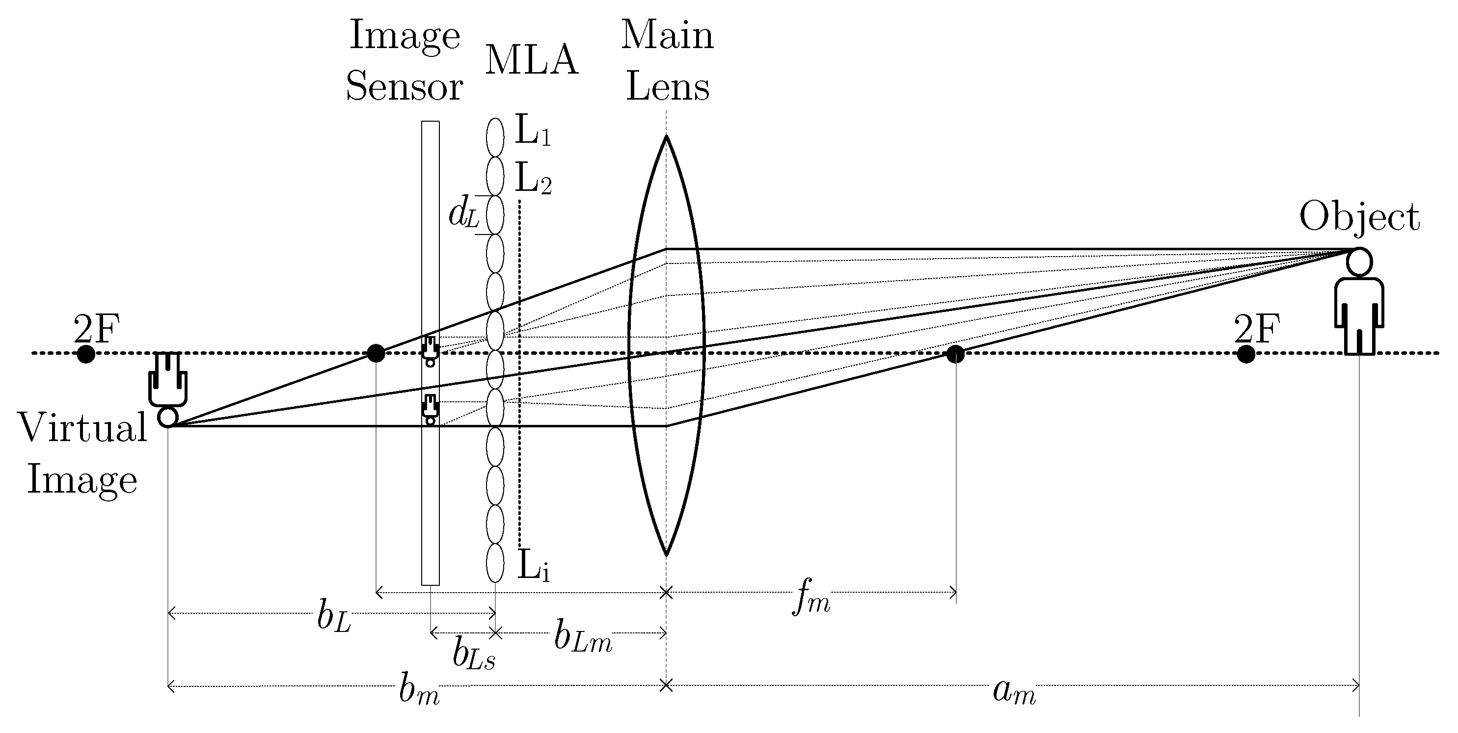
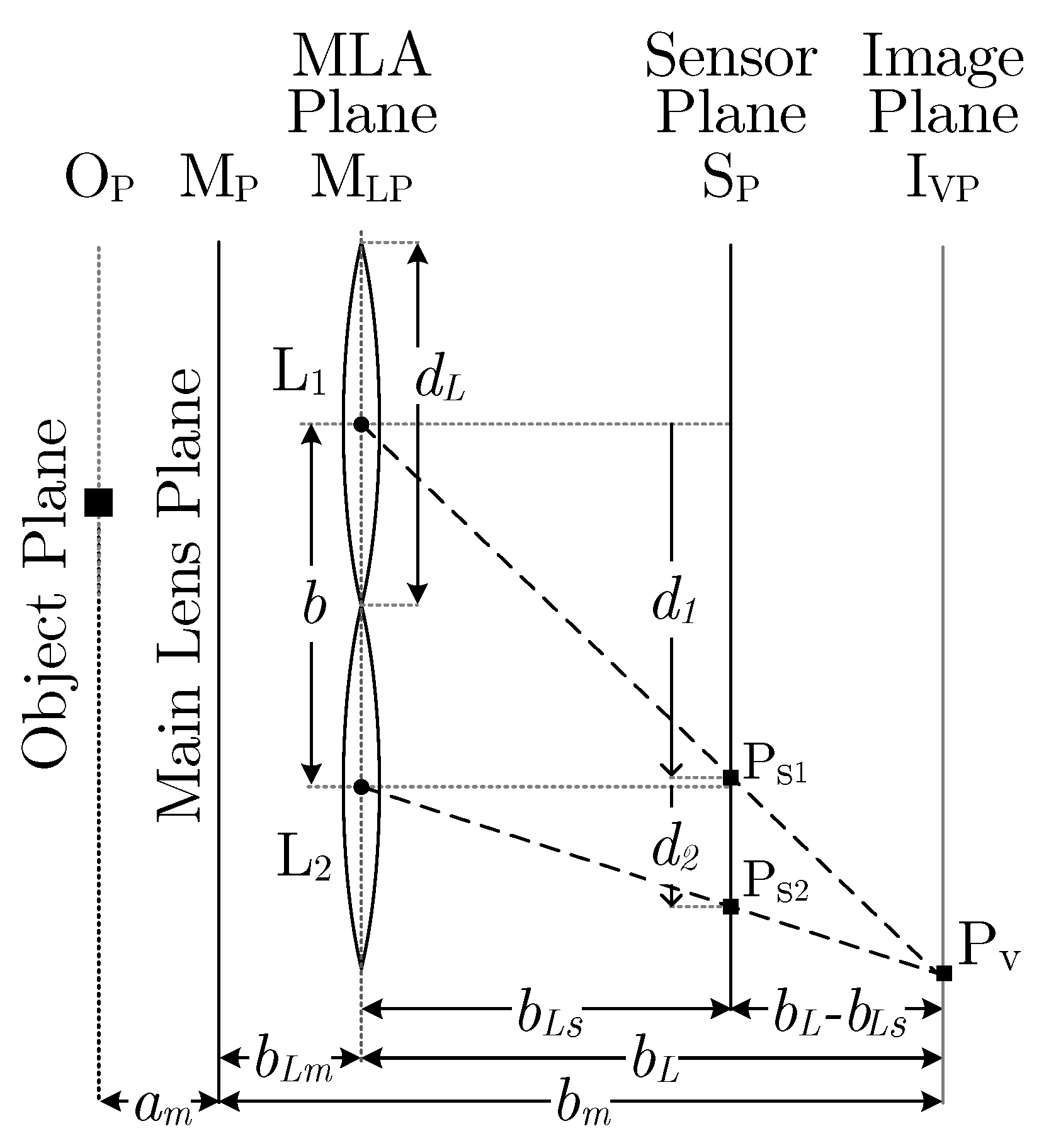
Plenoptic or light-field camera collects the light-field information of a scene by employing specialized design. Unlike the conventional camera, plenoptic camera captures light as well as associated direction information. It contains a micro-lens array (MLA) between the main lens and the image sensor [36], as depicted in Figure 1. Whereby represents a micro-lens in the grid with a unique identifier ; corresponds to the diameter of the micro-lens, is the focal length of the main lens, is the distance of the object from the main lens and is the distance between virtual image and the main lens. Moreover, is distance between MLA and the main lens, and is the distance of the corresponding virtual image from the MLA, is the distance between MLA and the image sensor. The image is formed behind the image sensor, hence it is virtual.
Within the plenoptic camera, a micro-lens in the MLA focuses a segment of main-lens image on the sensor with its own perspective. These micro-lenses either have similar focal lengths, or they consist of different focal lengths (multi-focus) [37]. Hence, each micro-lens captures a part of the scene corresponding to its position and perspective. As a result, an image that consists of a grid of micro-images with distinct perspectives is captured, as shown in Figure 2. As the scene is captured with several focal planes, the output image can be refocused even after it has been captured. In this way, a scene is recorded with several perspectives just by taking a single picture. Moreover, depth of the scene is computed by evaluating this data, that too can be estimated just by single recording of the scene. The depth-of-field (DOF) of the plenoptic camera is higher in comparison to same configuration conventional camera [7]. It also reduces occlusion regions [1] because of its large array of micro-lenses with small field view, which are closely interlaced together.
4. Depth Estimation Algorithm
The used single recording plenoptic camera based depth estimation algorithm is based on [6]. However, it is modified to completely exploit the advantages of the hardware realization. The modifications include the usage of a non-parametric transform and a respective cost function for finding the correspondence with minimum error.
In order to model the main camera thin lens camera model can be used:
In an MLA of the plenoptic camera, micro-lenses are arranged in a specific order, such as hexagonal. Due to such formation, a classic stereo camera paradigm can be considered for a pair of adjacent micro-lenses to calculate the depth of the scene, as shown in the Figure 3. Using the thin lens model, plenoptic camera is represented in 2D space as parallel planes: object plane , main lens plane , MLA plane , sensor plane and image plane . Two micro-lenses project points onto that is placed at the distance of from the . Rays from and intersect at virtual point onto the . Moreover, refers to the distance onto the from the principal axis of the respective , and b represents the baseline distance between the micro-lenses. The triangulation of this setup results in:
Whereby represents disparity that equals to: . The distance of , represented as virtual depth (v), is estimated with respect to intrinsic parameter of the camera that is calculated during the calibration process. Thus, v is computed by the relative distance of with respect to , which is only possible if the projected point is focused by minimum two micro-lenses.
The baseline distance between two adjacent micro-lenses equals to its diameter. So Equation (3) becomes:
By considering as a reference plane, 3D points can be represented as: center of a micro-lens , projection of a point onto , and the virtual point on . With the help of Thales’s theorem:
Similarly:
To calculate the actual distance of the object from the main lens, Equation (1) can be used by substituting , which results in:
Processing Steps
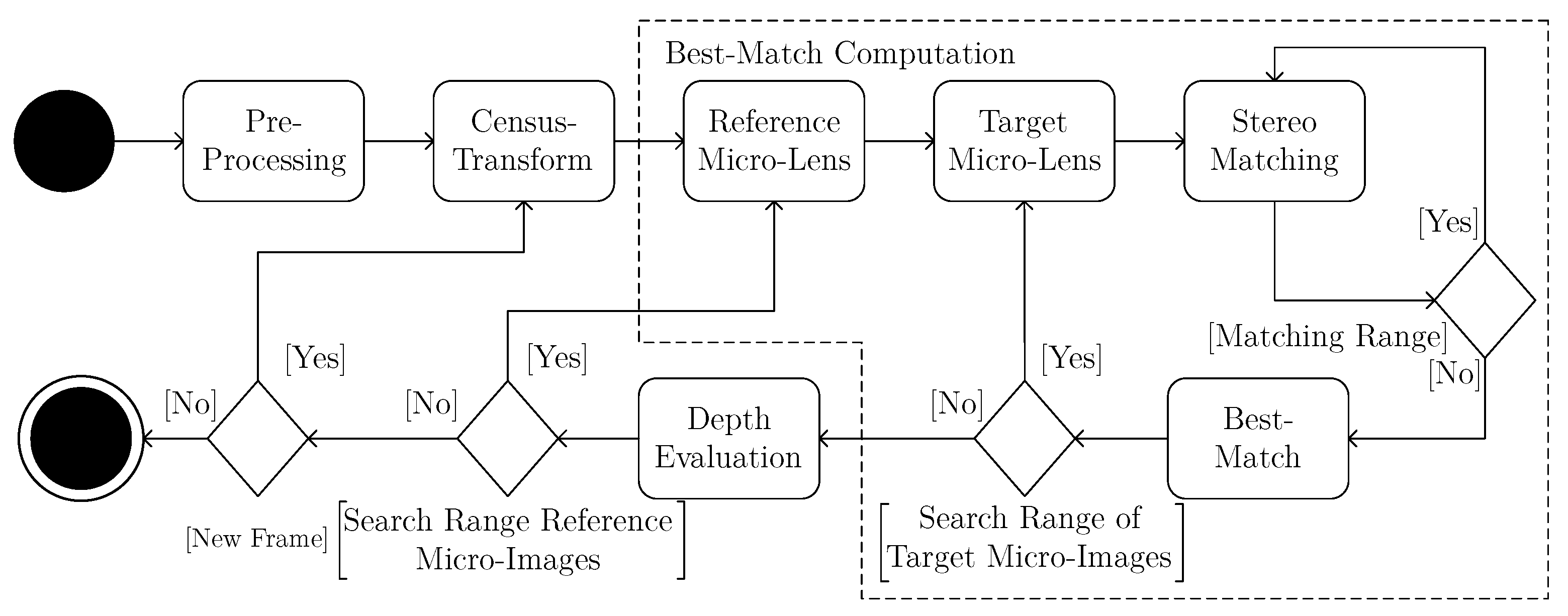
These equations show that the object distance is computed by estimating virtual depth which subsequently depends on the points projected by the micro-lenses. These calculations show how the final depth is estimated, which is achieved by a series of steps. Therefore, modified algorithm is divided into several processing steps: pre-processing, non-parametric transform, best-match computation and consequently depth-evaluation, as depicted by a UML activity diagram in Figure 4.
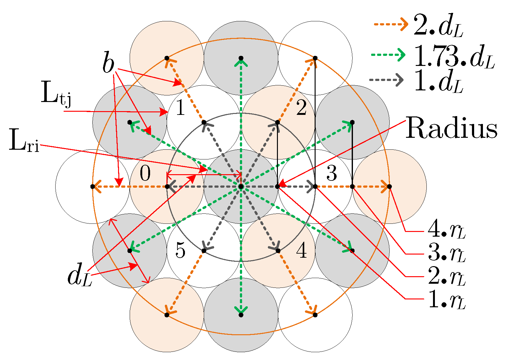
During pre-processing, geometric data of the micro-images, including lens-types and corresponding coordinates of its center, is calculated with the help of calibration information. Moreover, valid pixels in the input raw image are defined with respect to the MLA. Raytrix R5 camera [38] used in this study consists of an MLA with three different types of micro-lenses. Figure 5 depicts micro-lenses with distinct focal-lengths that are arranged in a hexagonal order. The center micro-lens and the surrounding micro-lenses are represented by and respectively. The numbers (0–5), which are inscribed on the micro-lenses correspond to the values of j in . Additionally, the radius of micro-lens , diameter and baseline distance b with respect to the are indicated. Since the micro-lenses are arranged in a hexagonal order and their respective diameters are equal, the b between two micro-lenses is computed by:
Whereby is a positive integer that implies how far is the target micro-lens from the in terms of number of micro-lenses, . However, it is only valid for the micro-lenses that are located at multiple of 60 with respect to the reference micro-lens. It is due to the hexagonal arrangement of the micro-lenses in the MLA grid. For instance, b of with the adjacent target micro-lens is calculated as:
The rest values of are calculated by using trigonometric relations.
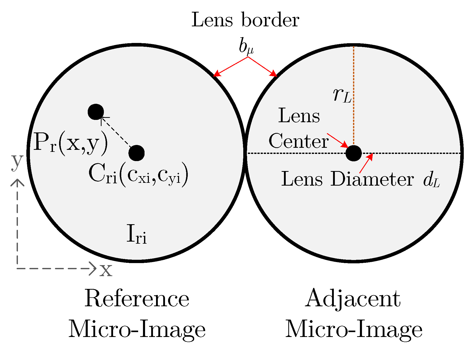
Figure 6 contains two adjacent micro-images. The border , and of the micro-images are defined in number of pixels. Raytrix R5 [38] camera has the of 1 pixel. The modified algorithm defines valid pixels in a micro-image which are those that lie within the border of the micro-lens. The reference pixel is placed inside the reference micro-image whose center is at . The point is considered valid only if this condition holds true:
The following step is to use a non-parametric transform on the input raw image. In the modified algorithm, census transform is employed. It depends on the relative order of the pixel intensities rather than the actual value of an intensity. This property makes it robust to illumination variations in an image. If a reference pixel is lying within neighborhood of , where , the census transform is formally defined as [39]:
Whereby, is the census transformed pixel, , is a comparison function and ⨂ denotes the bit wise concatenation.
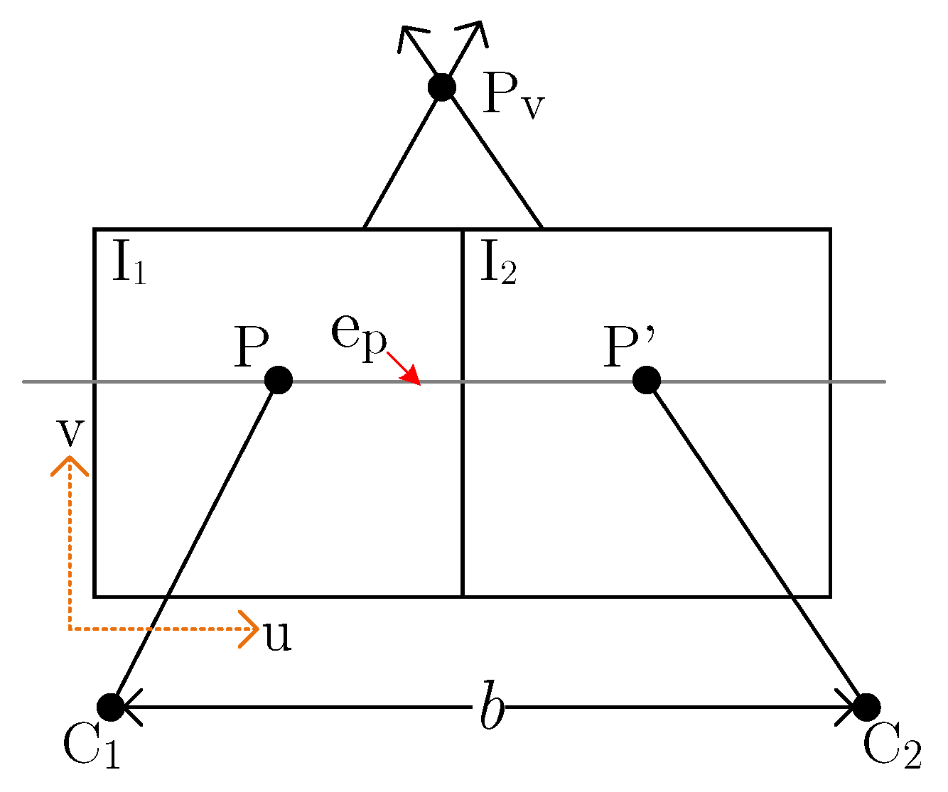
Best-match computation (BMC) involves finding the correspondence of valid census transformed reference pixel in target micro-images with a minimum error. This leads to the multi-view stereo problem, because every point of interest is projected by several micro-lenses. Correspondence is searched for a given of a reference micro-image in target micro-images . To save computation costs, search is restricted by matching only target pixels that lie on the epipolar lines within the neighborhood micro-images. Since the micro-lenses in the MLA are rectified and their respective planes are parallel, the epipolar line of a stereo pair is parallel to the b, as shown in Figure 7. A virtual point is projected on two adjacent micro-images planes and , at P and P’, with centers and respectively.
For each micro-image pair, stereo-matching is performed, the respective error is then subsequently compared. It results in a best-match for the given . The modified algorithm uses Hamming distance as the cost function to determine the error of similarity during the process of finding the correspondence. Along with the computation of best-match, respective disparity is computed. Finally, in depth-evaluation, virtual depth is estimated by using corresponding disparity and baseline distance of the best-match measurement.
5. Hardware System Design
FPGA’s inherently parallel architecture enables it to be used as a hardware accelerator to improve the performance from execution time perspective. Thus the objective is to exploit the available parallelization in the algorithm with respect to the hardware. It is achieved either by executing tasks concurrently with the help of multiple processing units or by pipelining the computational tasks. The former results in excessive use of available resources. Thus can only be used with a limited number of tasks and iterations. Pipelining increases the throughput of the given design. In ideal parallel program structure, pipelining initiation interval (ii) is 1, which means next input can be applied to the pipeline after one clock cycle. This way the pipeline stages are always busy and maximum possible throughput is achieved. Bigger values of ii correspond to the lower gain from the pipelining, for instance ii = n implies that pipeline stage stalls after each operation for (n − 1) clock cycle. There are various performance bottlenecks which restrict the associated gain from the parallelization.
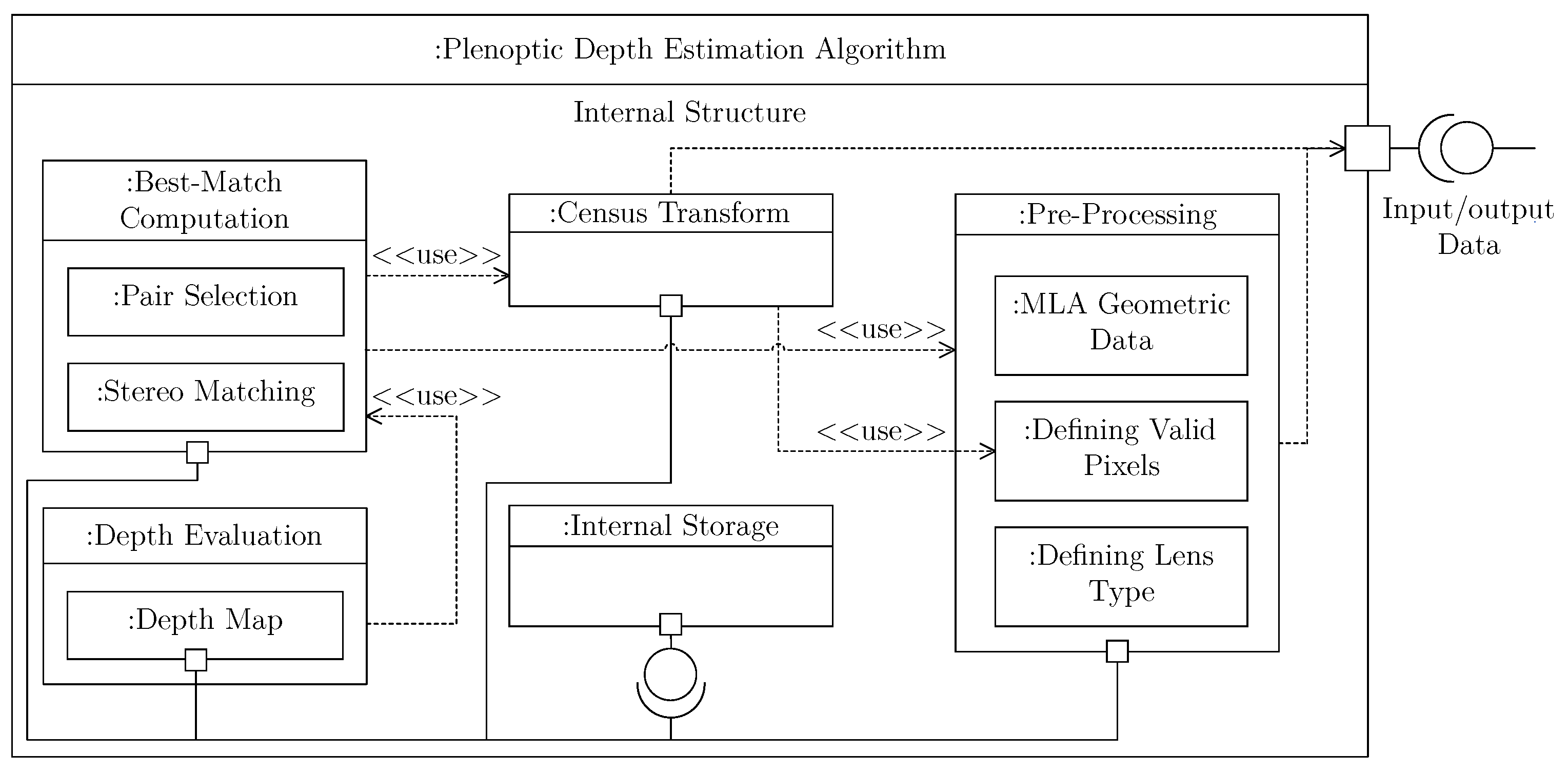
Sequential dependencies within the algorithm substantially limit the performance of the hardware. Therefore, it is essential in designing process to define all the sequential dependencies between internal sub-modules of the algorithm. Figure 8 illustrates the UML composite internal structure diagram that includes dependencies between different components of the algorithm. Each component (sub-modules) of the algorithm requires an interface with the external storage that retains the input and output data related to the algorithm. Similarly, these components also require an interface with internal storage to save their intermediate results. Depth-evaluation depends on best-match computation that can only start processing as soon as the pre-processing and non-parametric transform come to an end. For this reason, all three components cannot start executing independently. However, intra-component tasks can be executed in parallel, such as defining valid pixels and defining lens type are independent of each other and hence can run concurrently. The next sections explain how the algorithm is adapted and optimized with respect to the performance.
5.1. Bottleneck Segments
These are the segments of code that correspond to the largest tasks in the algorithm from the perspective of execution time. They, represented by , are the dominant performance bottlenecks in an algorithm. Whereby p corresponds to the sub-module of the algorithm and n is the number of the segment. They consist of either a portion or a complete sub-module. They contain a large number of complex operations or operations in a recursive order.
The respective bottleneck segments of the modified algorithm are arranged in Table 1. It shows that the most reside within the best-match computation sub-module of the algorithm. It is because of the recursive nature of the matching process. All of these are adapted and optimized with respect to the hardware.
5.2. Temporal Parallelization
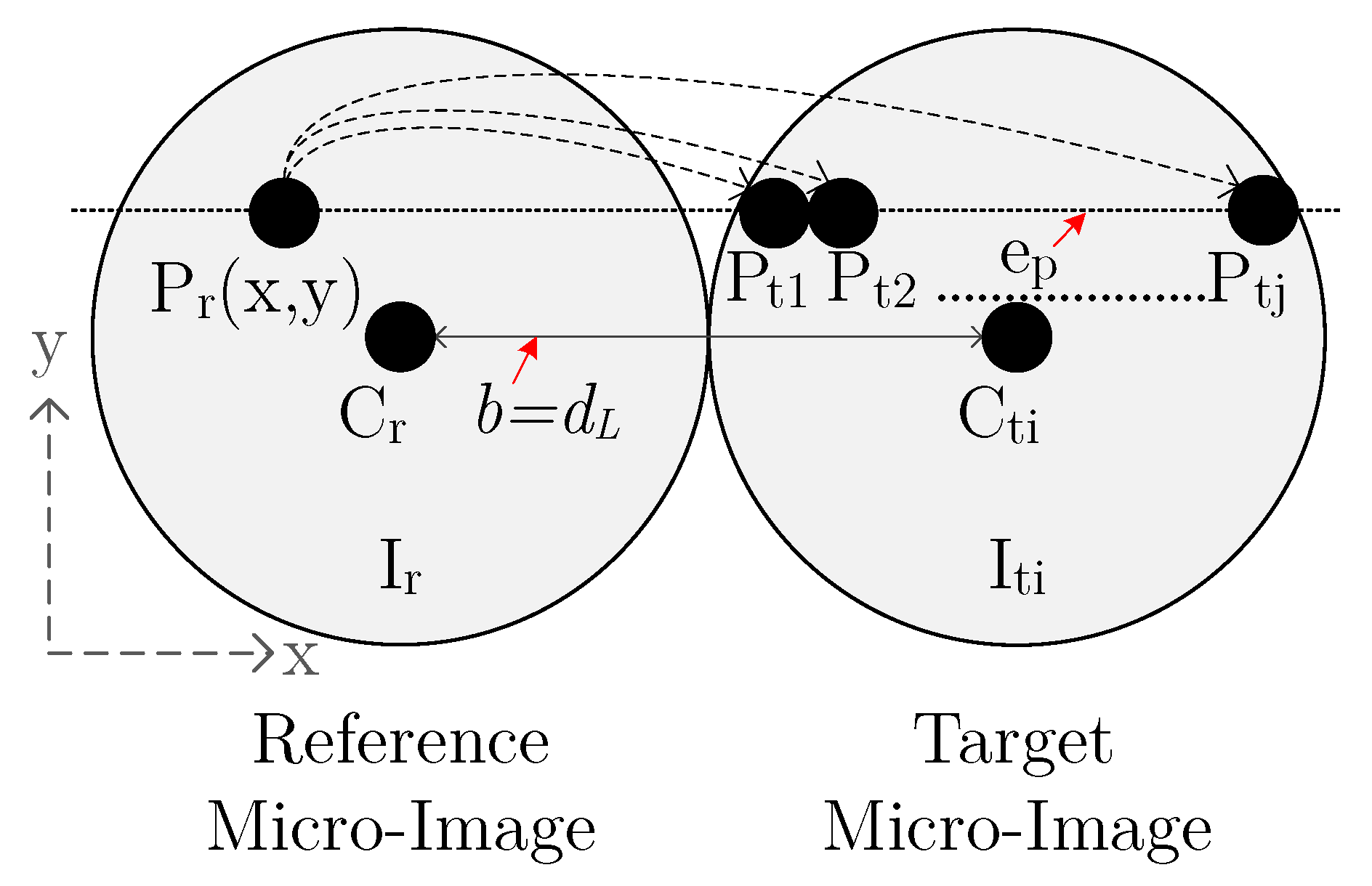
In proposed modified algorithm, selection of a pair for the stereo-matching depends on the baseline distance b. The different b with neighboring target micro-images from reference micro-image in an MLA is shown in Figure 9. During the stereo-matching process, to find the correspondence, needs to be correlated with several which are placed at b distance from the respective . Whereby b is calculated by Equation (10). The values inscribed in the micro-lenses refer to the of the respective baseline distance. The angles represent the arrangement of with respect to in the MLA.
Search process starts with target micro-images that are located at the shortest in all directions from . Subsequently, that is placed at higher b, is searched for a match. This way, baseline distance keeps increasing until a match is found. It is a computation intensive task due to its recursive nature. The modified algorithm reduces this effort by restricting the matching process. It is because the dimensions of the micro-images are quite small, e.g., of Raytrix R5 camera is almost 23 pixels. It only allows each micro-image to capture a little fraction of information. Therefore, it can be established that the probability of finding the match is higher in the micro-images which are located in close proximity to the . By taking it into account, it is determined from experiments that a good match is found with , which is located within range of from . Thus the maximum baseline distance is restricted to .
From Figure 9, it is apparent that the matching occurs in all directions with respect to the . However, it causes redundant matching computations to take place, because in subsequent stereo-matching the role of same pair gets swapped, i.e., reference with target micro-image. For this reason, the proposed design allows only those micro-images to be correlated during the stereo-matching, which are located between from the reference micro-image. It ensures matching to be carried out only once for each pair, and therefore it significantly reduces the redundant computations. In this formation, maximum number of target micro-images that can be correlated with is .
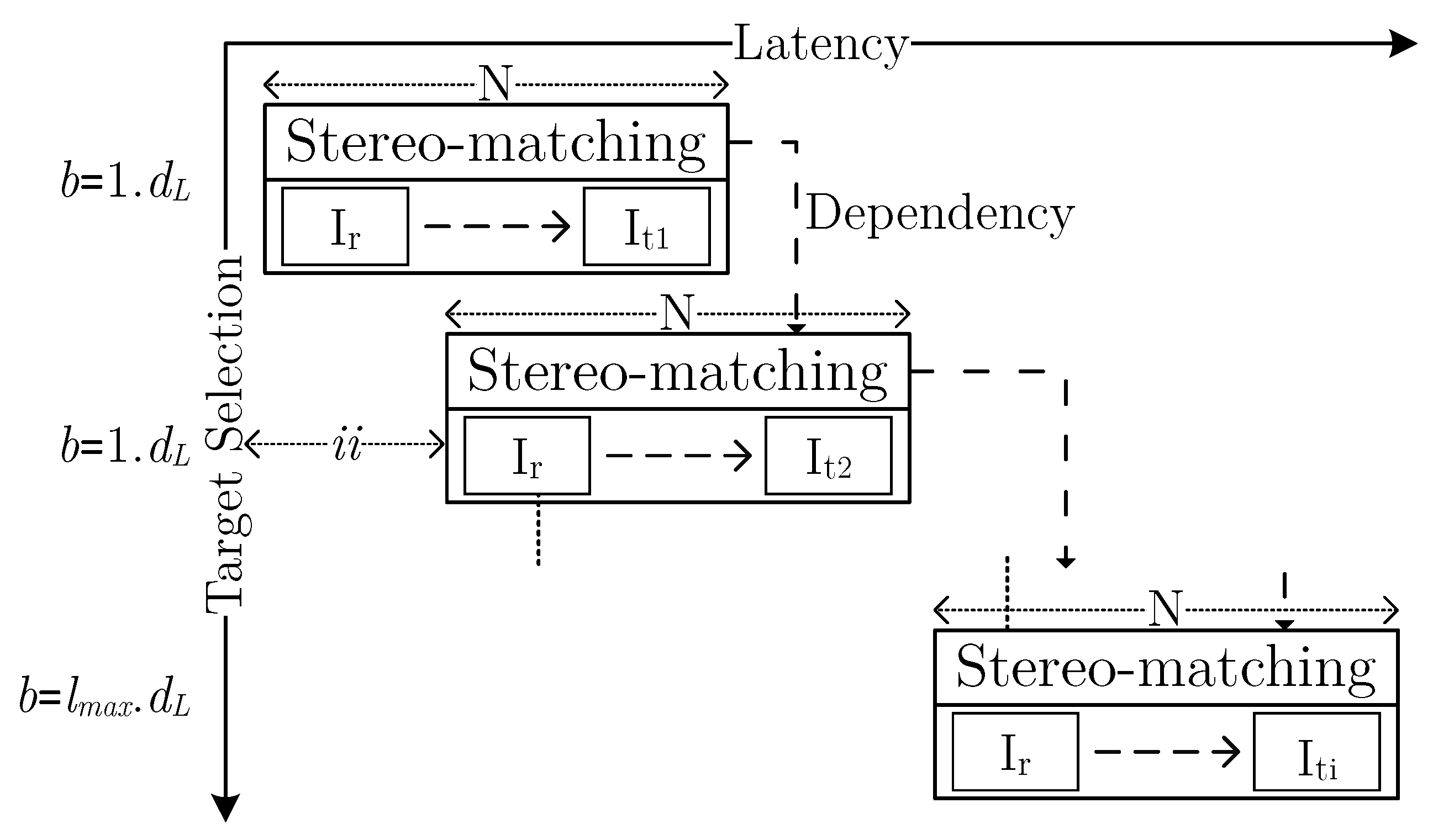
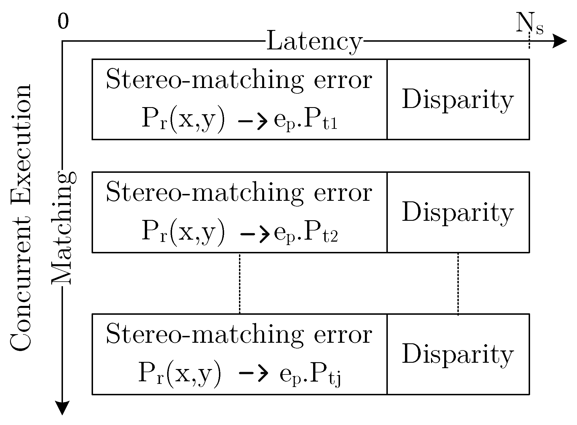
Selection of micro-image pairs to find the best match is pipelined, as depicted in Figure 10. Whereby N corresponds to the latency of one matching task. The temporal parallelization ensures the extensive search for the match to be carried out concurrently. Total latency of stereo-matching with number of target micro-images, without the pipelining is clock cycles, and with pipelining it equals to ii clock cycles. Thereby, gain obtained from temporal parallelization is restricted by the value of ii. In stereo-matching, to save computation, a condition is added which ensures that matching only occurs with that are placed at higher distance () if a match is found at the shorter distance. Thus, in a case, when no match is found at the shortest distance, search stops and the next reference pixel is selected. This however, results in inter-iteration (loop-carried) dependency that consequently increases .
5.3. Spatial Parallelization
Finding the best match is a nested stereo-matching process, as shown in Figure 11. After selecting a target micro-image with respect to , matching is performed within its physical boundaries. Epipolar geometry is employed in the design in order to reduce the computation efforts. The maximum number of pixels, represented by M, that can lie on an epipolar line is equal to the diameter of the micro-lens minus its border . For Raytrix R5 camera, M is calculated to 22 using following equation:
From Figure 11, it is clear that matching process is recursive in nature. It therefore enables the proposed design to use the spatial parallelization, as depicted in Figure 12. Each correlation with target micro-image pixel computes error of stereo-matching and corresponding disparity. If the latency of each comparison is clock cycles, the total latency to finish the matching process of hardware which ensures concurrency is ideally clock cycles.
5.4. Census Transform
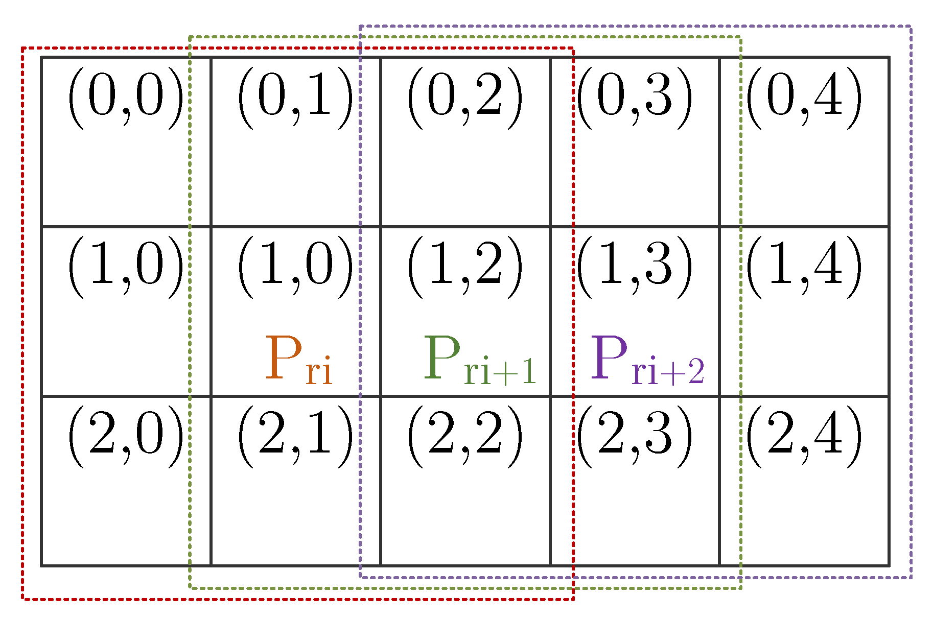
Census transform used in the design is adapted to exploit parallelization. Figure 13 shows a segment of an image where pixels are arranged in rows and columns (3 × 5). In this case, window size for the census transform is set to: M × M = 3 × 3. The process starts by selecting center pixel that is correlated with the surrounding pixels within the respective window. In the next iteration, window shifts to right and the next center pixel is selected and process goes on. These windows are represented by dotted lines and distinct colors. This process is completely pipelined in the proposed design, which allows iterations to run concurrently. Moreover, in hardware design, resource usage is optimized by using the arbitrary width data type. The corresponding number of bits is set to: . The inter-iteration dependencies are resolved by using a buffer of depth to store the bit comparison results during the correlation process.
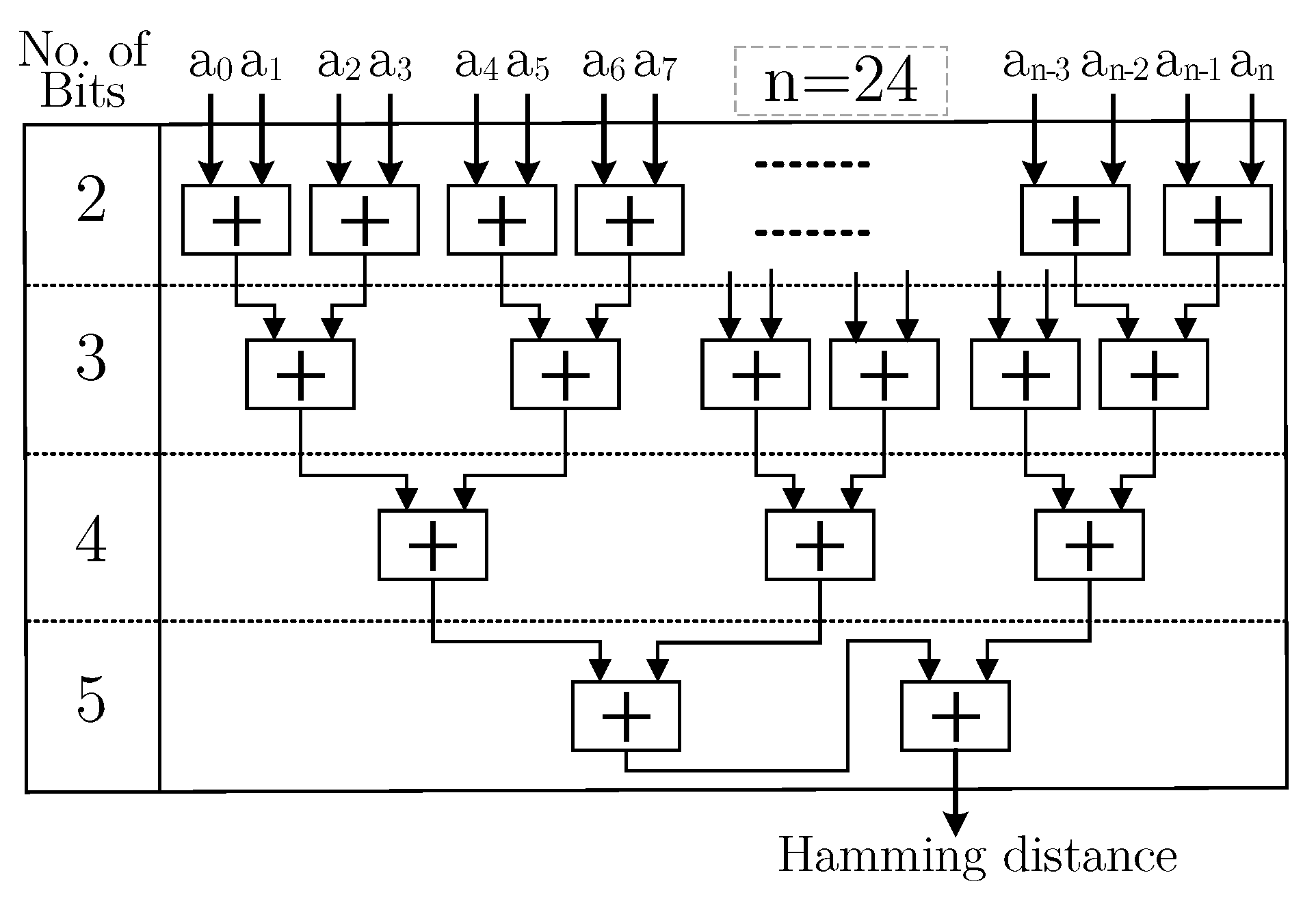
Hamming distance is well established as a cost function for census transform. It is calculated for a target range and it results in dissimilarity between a pair of pixels. The pixel with the minimum Hamming distance corresponds to the best match for a given pixel . For a window census transform, the number of bits n (bit length) of each transformed pixels is . Sequential realization of Hamming distance implements long carry chains of the adders. The optimized hardware solution is a balanced tree implementation that uses adders with arbitrary number of bits for intermediate results, as shown in Figure 14. It consequently reduces the resource consumption. Total number of required adders are: . This figure shows the realization of a 5 × 5 census transform window, so the bit length of pixels is 24, and the total number of adders required are 23. Maximum number of bits m for the adder is calculated by , which is equal to or greater than n, so in this case m is 5. This implementation only requires two clock cycles to produce the results, which includes operations: comparing bits (XOR), shifting right, sum of the set bits and in the end a comparison to check if it is the minimum distance and calculating the corresponding disparity.
5.5. Memory Optimizations
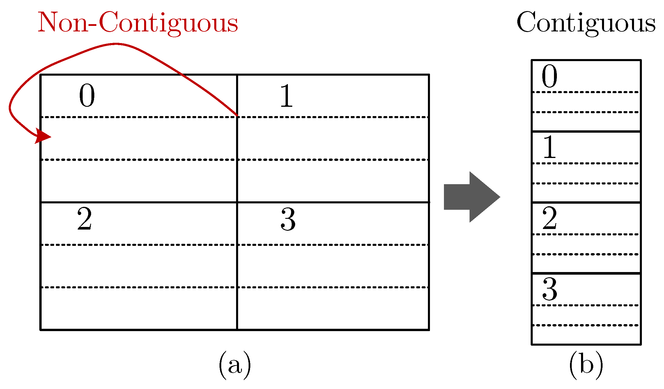
The optimization of the hardware design is an iterative process. The major challenge lies in management of the memory accesses. Since the modified algorithm consists of a substantial number of computation operations, a large number of low latency memory cells are required to store the corresponding results. However, only limited such memory is available in a given FPGA based SoC. External DDR memory can be used but accessing such memory is costly with respect to the execution time. Thus a large number of memory accesses eventually increase the latency of the algorithm exponentially. The proposed algorithm design resolves this by partitioning the input raw image into several segments and process them from the DDR memory in parallel. This ensures concurrent access. The input image data are stored in the memory in a row-major order. The process to find the best match for a given pixel occurs in both directions, i.e., horizontal and vertical. Therefore, the image data are partitioned into smaller blocks. However, it makes the order of the data non-contiguous that is stored in a respective block, as shown in the Figure 15a. It is resolved by rearranging the blocks to ensure that the stored data are contiguous (see Figure 15b).
Moreover, low latency memory cells are exploited during the matching process to comply with timing constraints. It is realized in conjunction with a lookup table, which stores the corresponding validity information of the pixels. A certain number of low latency memory cells are allocated to buffer the data from the external DDR memory. These data are repeatedly used in one iteration of the operations and therefore saves a large number of high cost external memory accesses.
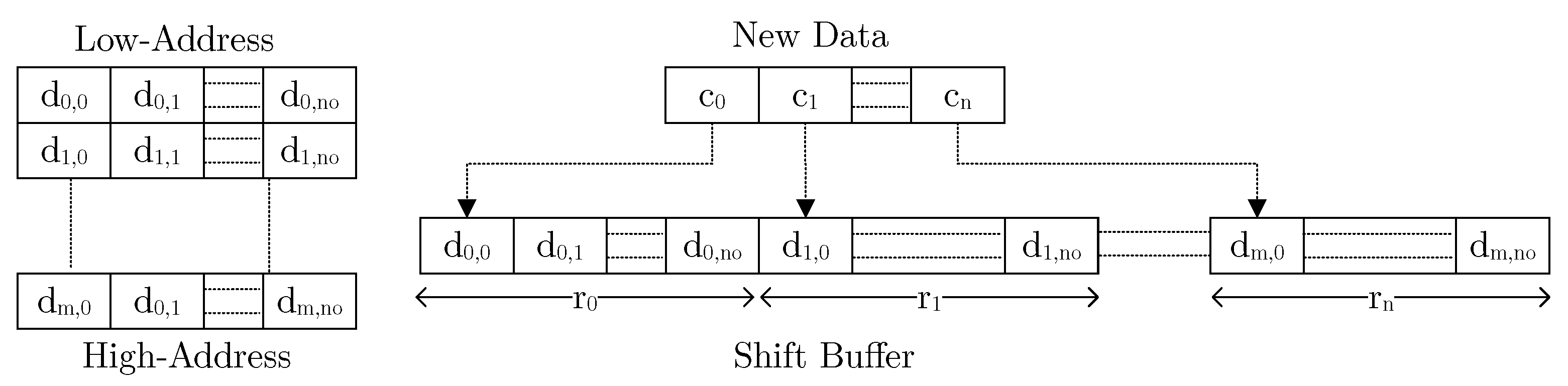
Furthermore, a circular shift-buffer based on low latency memory is designed for the algorithm. As explained earlier, in stereo-matching, the micro-images are selected which lie on the epipolar line, and the baseline distance to choose target micro-images is restricted to 4. Thus in matching process, the same data are accessed multiple times because each pixel needs to be compared with the target micro-image. It establishes the ground to utilize the available memory in an optimized order by removing the redundant memory accesses. The idea is to perform stereo-matching with respect to rows and add the new input data from the external memory only when all the pixels placed on the first column of the buffer finish their respective matching. The memory is arranged from low to high addresses, as shown in left side of the Figure 16. The input data size is R × C, so the buffer size is chosen R ×. Whereby equals to a scalar value that is specified with respect to the available memory. The value of is set 92 in the implementation, because 4 micro-images are considered for the matching whose respective diameter is 23 pixels (Raytrix R5 camera). The data are arranged with respect to rows. When the succeeding column from input image requires to be written in the buffer, the pointer shifts right and the first element of each row is replaced by the respective new data. Subsequently, the shift-counter is increased by one. In this case, index of the buffer to access the last element is equal to the zeroth element index minus the shift-counter.
6. Evaluation and Results
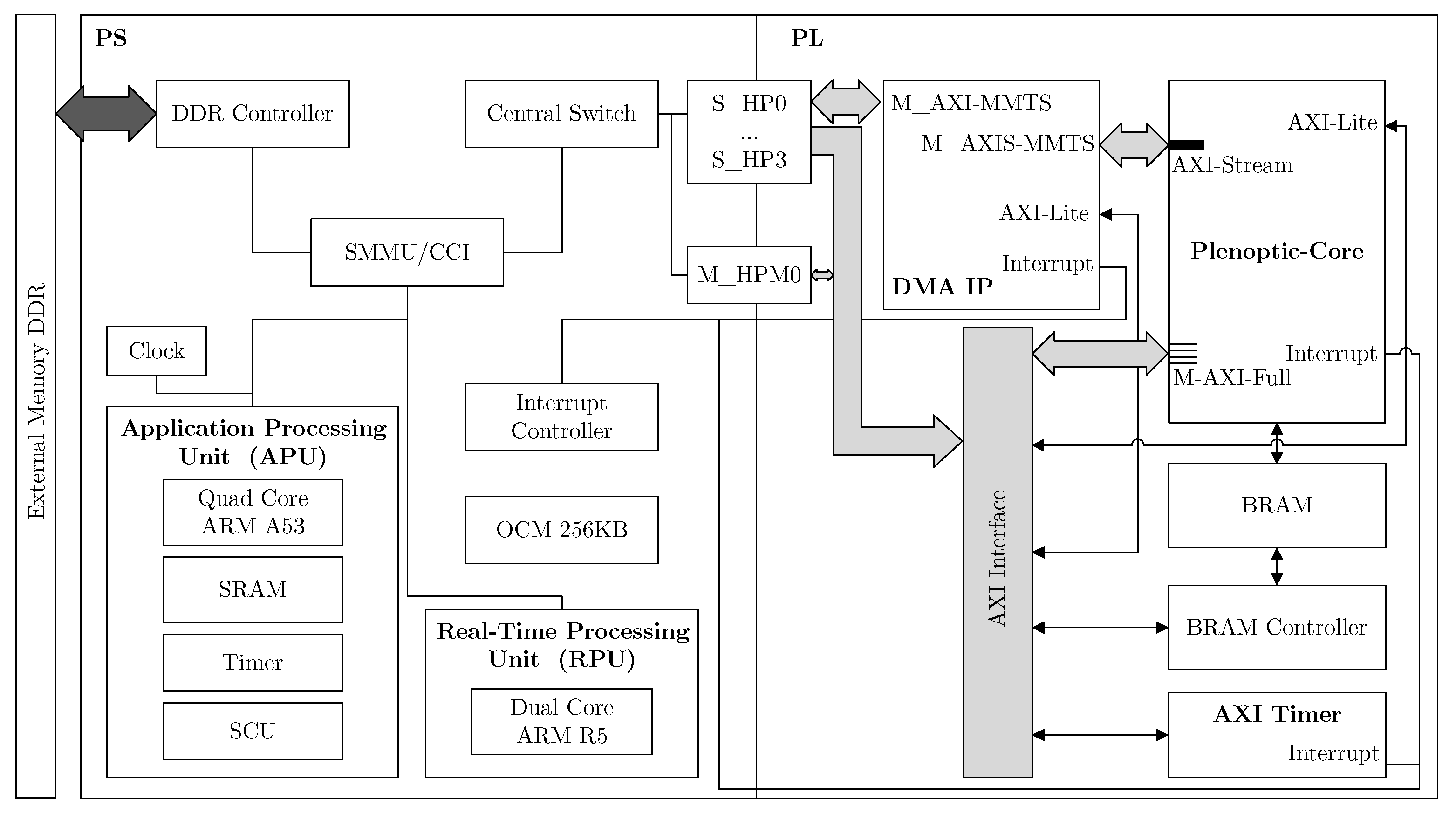
In the proposed design, FPGA is configured as a co-processor where it is not directly connected with an image acquisition logic. The hardware architecture for selected plenoptic camera based algorithm is presented in Figure 17. It is based on Xilinx Zynq UltraScale+ MPSoC that is divided mainly into processing system (PS) and programmable logic (PL). PS consists of a quad-core ARM processor, a dual core real-time ARM processor, a general interrupt controller, memory interfaces and on-chip-memory (OCM). PL contains FPGA configurable logic blocks, resources such as lookup tables (LUTs) and flip-flops (FFs). Furthermore, it contains DSP blocks and Block RAMs (BRAMs). Programmable logic and processing system communicates via high performance (HP) master/slave ports and accelerator coherency port (ACP). Plen-Module represents the depth estimation algorithm module in the system. It is connected with the application processor unit (APU) via AXI_Lite interface and master HP0 port. This interface is responsible for configuring and initializing the module. HP ports are connected directly to the external memory. Plen-Module utilizes available slave HP ports to communicate with memory for reading input data and storing output data. Intermediate results are stored in the BRAM. APU can read BRAM with the help of BRAM controller. Furthermore, Plen-Module is also connected with interrupt controller. Similarly, AXI_Timer is coupled with RPU via AXI_Lite interface. It is used for timing measurement.
The hardware design was realized with the help of Xilinx Vivado High-level synthesis (HLS) tool. It was implemented on Xilinx Zynq UltraScale+ ZCU102 programmable MPSoC with following parameters:census window size was 5 × 5, the range of Hamming distance matching was set to of micro-image that is 23 and the input image resolution was: 512 × 512. The RTL of the algorithm was generated via Xilinx HLS which was then incorporated in the system architecture using Xilinx Vivado design suite. For light-field images, few synthetic datasets are available, such as [40,41]. However, neither of them contain raw micro-images and therefore are not suitable for the presented algorithm. For this reason, a dataset was recorded focusing on indoor scenarios with the help of Raytrix R5 camera. The resulting sparse depth maps from the presented algorithm were correlated with the depth maps generated by the RxLive software (Raytrix GmbH [38]). The camera was considered to be calibrated and therefore same geometric parameters (i.e., lens type, validity) were used for all the test benches. The evaluation metric was execution time of the algorithm to calculate the depth map.
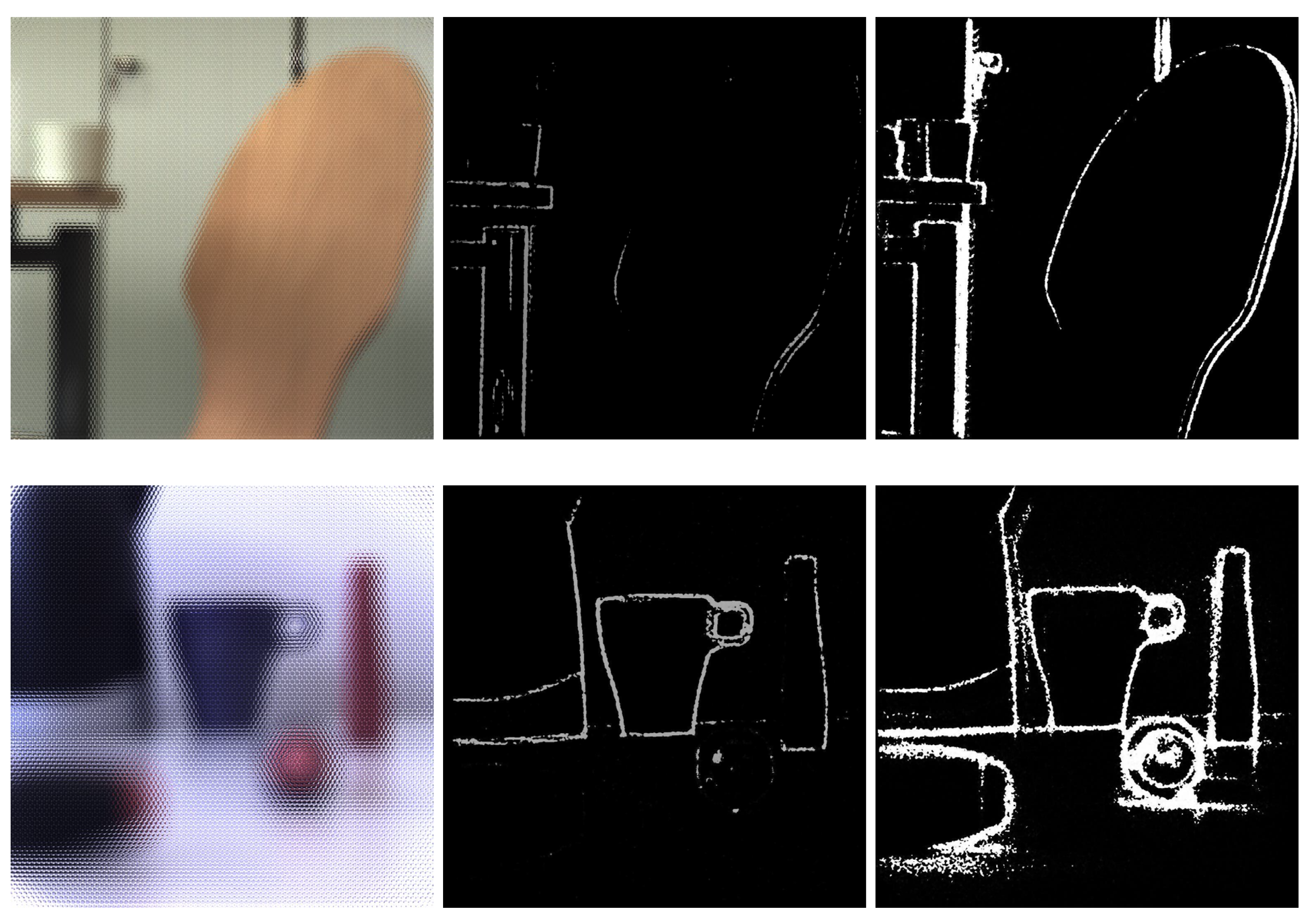
Figure 18 shows two different scenes captured by the camera. The top dataset () represents an indoor scenario consisting of a table and a chair from the perspective of the wheeled walker, whereas the bottom one () depicts objects closer to the camera. Images are arranged as follows: (from left to right) raw image consisting of micro-images, depth map calculated by RxLive and the depth map generated by the presented algorithm. From the figure, it is clear that the latter’s depth map was more dense than the RxLive. The quantitative results calculated by image statistics are listed in the Table 2. The density was computed by dividing the total number of valid depth pixels with the total number of pixels in the given area. It shows that the density of the depth maps estimated by presented algorithm for dataset was ≈52 times more, and for dataset was ≈7 times more than the respective RxLive depth maps. Similarly, presented algorithm’s depth map density for dataset was ≈31% more, and for dataset is ≈21% higher than the respective Zeller et al. [6] depth maps. Moreover, the standard deviation of the depth maps from RxLive was slightly better than the presented algorithm.
The initial implementations of the design were not able to meet the timing constraints, such as setup time. Moreover, the latency of first implementable design was more than 1 hour. However, after repeatedly improving the system, the latency dropped and timing constraints were met. The actual execution time of the algorithm measured in milliseconds with respect to different optimizations is arranged in Table 3. in the first column of the table refers to the bottleneck segments listed in Table 1, whereas optimization corresponds to the approaches described in Section 5. Hence, the group of both represents the optimization used at specific . Moreover, this table includes the maximum latency obtained from Xilinx HLS as well as the utilization results acquired from Xilinx Vivado design suite. The utilization was measured by the consumption of LUTs, FFs, BRAMs and DSPs. To measure the accuracy of the results, percentage of bad pixels (BPR) that corresponded to the error ≥1 and the absolute relative error were used. The maximum achieved clock frequency that met implementation timing constraints was 200 MHz.
, and were adapted to use the temporal parallelization, and the respective execution time of the algorithm consequently dropped to 1121.25 ms. Similarly, temporal parallelization on and resulted in gain of 394.24 and 122.89 ms respectively. The execution time was further reduced by using spatial parallelization on and . The combination of temporal and spatial parallelization on , and caused the execution time to dramatically decrease to 334.41 ms. Subsequently, Hamming distance optimization together with arbitrary length fixed point numbers shrank down the execution time by ≈8%, which was at the cost of ≈3% additional LUTs, almost twice the BRAMs and ≈20 times more DSPs, whereas the FFs consumption was slightly improved by ≈0.25%. The overall resource usage increased due to the length of the fixed point numbers. Finally, memory optimization brought the execution time down to 27.18 ms. The corresponding gain was 283.92 ms, whereas the number of BRAMs raised to 1797 that corresponded to ≈98.5% utilization.
The presented algorithm was additionally adapted, optimized, implemented and tested on a mobile GPU. It was achieved by refining bottleneck segments to exploit parallelization. The algorithm was realized using CUDA programming model. The respective specification of each execution platform employed in the evaluation process is listed in Table 4. The comparison of executing the modified single recording algorithm on the PC-system, on mobile GPU based system and on FPGA MPSoC is arranged in Table 5. The GPU was configured in 6-core 15 watt mode. The power consumption was calculated by measuring the current drawn and voltage with the help of digital multimeter (Protek 506). FPGA hardware was ≈20% faster than mobile GPU and ≈69% faster than the PC-system. Consequently, it provided highest fps and consumed the least power as compared to both mobile GPU and PC-system. From these results, it can be concluded that the presented FPGA design was a suitable solution for the targeted mobile application.
7. Conclusions
Depth estimation algorithms are used in various fields, such as in research and automation. This paper proposes a plenoptic based approach which works on a single recording of a raw image from the light-field camera. From the timing point of view, high computation tasks and large resulting execution time are the biggest challenges of such algorithms. The existing solution is to use a GPU based system with high computation power to comply with the computation requirements. However, this solution is expensive from power consumption perspective and therefore cannot be used in power limited applications, such as a mobile application. This paper proposes a modified single recording plenoptic camera based depth estimation algorithm. Moreover, it presents a FPGA based hardware design in order to optimize the performance of the algorithm by employing inherited parallelization. FPGA based hardware exploits both temporal and spatial parallelization in the targeted algorithm. The performance bottleneck is mainly caused by the presence of recursive operations and large memory access time. Optimization of memory accesses and managing the resources is a complex and an iterative process. The presented hardware design is realized and compared with the low-power mobile GPU solution. The results have shown a considerable improvement in the performance with respect to execution time. It leads to the conclusion that the presented FPGA hardware design is faster and consumes less power as compare to both PC-system and mobile GPU based solutions.
Author Contributions
Conceptualization, F.B. and T.G.; methodology, F.B. and T.G.; software, F.B.; validation, F.B.; formal analysis, F.B. and T.G.; investigation, F.B.; resources, F.B.; data curation, F.B.; writing—original draft preparation, F.B.; writing—review and editing, F.B. and T.G.; visualization, F.B. and T.G.; supervision, T.G.; project administration, T.G.; funding acquisition, T.G. All authors have read and agreed to the published version of the manuscript.
Funding
This work is financed by the Baden-Württemberg Stiftung gGmbH, Germany.
Institutional Review Board Statement
Not applicable.
Informed Consent Statement
Not applicable.
Data Availability Statement
Not applicable.
Conflicts of Interest
The authors declare no conflict of interest.
Abbreviations
The following abbreviations are used in this manuscript:
| ACP | Accelerator Coherency Port |
| APU | Application Processor Unit |
| ASIC | Application-specific Integrated Circuit |
| BPR | Percentage of Bad Pixels |
| BRAM | Block RAM |
| CPU | Central Processing Unit |
| CT | Census Transform |
| DOF | Depth of Field |
| FF | Flip-flop |
| GPU | Graphics Processing Unit |
| HLS | High-level Synthesis |
| ii | Initiation Interval |
| LUT | Lookup Table |
| MLA | Micro-lens Array |
| OCM | On-chip-memory |
| PL | Programmable Logic |
| PS | Processing System |
| RMSE | Root-mean-square Error |
References
- Adelson, E.H.; Wang, J. Single lens stereo with a plenoptic camera. IEEE Trans. Pattern Anal. Mach. Intell. 1992, 14, 99–106. [Google Scholar] [CrossRef] [Green Version]
- Fiss, J.; Curless, B.; Szeliski, R. Refocusing plenoptic images using depth-adaptive splatting. In Proceedings of the 2014 IEEE International Conference on Computational Photography (ICCP), Santa Clara, CA, USA, 2–4 May 2014; pp. 1–9. [Google Scholar] [CrossRef]
- Vaish, V.; Wilburn, B.; Joshi, N.; Levoy, M. Using plane + parallax for calibrating dense camera arrays. In Proceedings of the 2004 IEEE Computer Society Conference on Computer Vision and Pattern Recognition, Washington, DC, USA, 27 June–2 July 2004; pp. 2–9. [Google Scholar] [CrossRef]
- Yang, J.C.; Everett, M.; Buehler, C.; McMillan, L. A Real-time distributed light field camera. In Proceedings of the 13th Eurographics Workshop on Rendering; Eurographics Association: Aire-la-Ville, Switzerland, 2002; pp. 77–86. [Google Scholar]
- Bizai, G.; Peiretti, F.; Salvatelli, A.; Drozdowicz, B. Algorithms for codification, multiperspective and refocusing of light fields: Implementation and evaluation. In Proceedings of the 2017 XLIII Latin American Computer Conference (CLEI), Cordoba, Argentina, 4–8 September 2017; pp. 1–7. [Google Scholar] [CrossRef]
- Zeller, N.; Quint, F.; Stilla, U. Establishing a probabilistic depth map from focused plenoptic cameras. In Proceedings of the 2015 International Conference on 3D Vision, Lyon, France, 19–22 October 2015; pp. 91–99. [Google Scholar] [CrossRef]
- Perwass, C.; Wietzke, L. Single lens 3D-camera with extended depth-of-field. In Human Vision and Electronic Imaging XVII; Rogowitz, B.E., Pappas, T.N., de Ridder, H., Eds.; International Society for Optics and Photonics (SPIE): Bellingham, WA, USA, 2012; Volume 8291, pp. 45–59. [Google Scholar] [CrossRef] [Green Version]
- Zeller, N. Direct Plenoptic Odometry-Robust Tracking and Mapping with a Light Field Camera. Ph.D. Thesis, Technische Universität München, München, Germany, 2018. Available online: https://dgk.badw.de/fileadmin/user_upload/Files/DGK/docs/c-825.pdf (accessed on 17 June 2021).
- Collange, S.; Defour, D.; Tisserand, A. Power Consumption of GPUs from a Software Perspective. In Proceedings of the International Conference on Computational Science, Baton Rouge, LA, USA, 25–27 May 2009; Springer: Berlin/Heidelberg, Germany, 2009; pp. 914–923. [Google Scholar] [CrossRef] [Green Version]
- Engel, G.; Bhatti, F.; Greiner, T.; Heizmann, M.; Quint, F. Distributed and context aware application of deep neural networks in mobile 3D-multi-sensor systems based on cloud-, edge- and FPGA-computing. In Proceedings of the 2020 IEEE 7th International Conference on Industrial Engineering and Applications (ICIEA), Bangkok, Thailand, 16–21 April 2020; pp. 993–999. [Google Scholar] [CrossRef]
- Wang, G.; Xiong, Y.; Yun, J.; Cavallaro, J.R. Accelerating computer vision algorithms using OpenCL framework on the mobile GPU—A case study. In Proceedings of the IEEE International Conference on Acoustics, Speech and Signal Processing (ICASSP), Vancouver, BC, Canada, 26–31 May 2013; IEEE: Piscataway, NJ, USA, 2013; pp. 2629–2633. [Google Scholar] [CrossRef] [Green Version]
- Rister, B.; Wang, G.; Wu, M.; Cavallaro, J.R. (Eds.) A Fast and Efficient Sift Detector Using the Mobile GPU. In Proceedings of the 2013 IEEE International Conference on Acoustics, Speech and Signal Processing, Vancouver, BC, Canada, 26–31 May 2013. [Google Scholar]
- Amara, A.; Amiel, F.; Ea, T. FPGA vs. ASIC for low power applications. Microelectron. J. 2006, 37, 669–677. [Google Scholar] [CrossRef]
- Kuon, I.; Rose, J. Measuring the Gap Between FPGAs and ASICs. IEEE Trans. Comput. Aided Des. Integr. Circuits Syst. 2007, 26, 203–215. [Google Scholar] [CrossRef] [Green Version]
- Page, D.S. A Practical Introduction to Computer Architecture; Texts in Computer Science; Springer: Dordrecht, The Netherlands; London, UK, 2009. [Google Scholar]
- Johnston, C.T.; Gribbon, K.T.; Bailey, D.G. Implementing Image Processing Algorithms on FPGAs. Available online: https://crisp.massey.ac.nz/pdfs/2004_ENZCON_118.pdf (accessed on 17 June 2021).
- Downton, A.; Crookes, D. Parallel architectures for image processing. Electron. Commun. Eng. J. 1998, 10, 139–151. [Google Scholar] [CrossRef]
- Xu, Y.; Long, Q.; Mita, S.; Tehrani, H.; Ishimaru, K.; Shirai, N. Real-time stereo vision system at nighttime with noise reduction using simplified non-local matching cost. In Proceedings of the 2016 IEEE Intelligent Vehicles Symposium (IV), Gothenburg, Sweden, 19–22 June 2016; pp. 998–1003. [Google Scholar] [CrossRef]
- Wang, W.; Yan, J.; Xu, N.; Wang, Y.; Hsu, F.H. Real-Time High-Quality Stereo Vision System in FPGA. IEEE Trans. Circuits Syst. Video Technol. 2015, 25, 1696–1708. [Google Scholar] [CrossRef]
- Draper, B.A.; Beveridge, J.R.; Bohm, A.; Ross, C.; Chawathe, M. Implementing image applications on FPGAs. Object recognition supported by user interaction for service robots. IEEE Comput. Soc. 2002, 3, 265–268. [Google Scholar] [CrossRef] [Green Version]
- Sugimura, T.; Shim, J.; Kurino, H.; Koyanagi, M. Parallel image processing field programmable gate array for real time image processing system. In Proceedings of the 2003 IEEE International Conference on Field-Programmable Technology (FPT) (IEEE Cat. No.03EX798), Tokyo, Japan, 17 December 2003; pp. 372–374. [Google Scholar] [CrossRef]
- Jinghong, D.; Yaling, D.; Kun, L. Development of image processing system based on DSP and FPGA. In Proceedings of the 2007 8th International Conference on Electronic Measurement and Instruments, Xi’an, China, 16–18 August 2007; pp. 2-791–2-794. [Google Scholar] [CrossRef]
- Birla, M. FPGA based reconfigurable platform for complex image processing. In Proceedings of the 2006 IEEE International Conference on Electro/Information Technology, East Lansing, MI, USA, 7–10 May 2006; pp. 204–209. [Google Scholar] [CrossRef]
- Bhatti, F.; Greiner, T.; Heizmann, M.; Ziebarth, M. A new FPGA based architecture to improve performance of deflectometry image processing algorithm. In Proceedings of the 2017 40th International Conference on Telecommunications and Signal Processing (TSP), Barcelona, Spain, 5–7 July 2017; pp. 559–562. [Google Scholar] [CrossRef]
- Michailidis, G.T.; Pajarola, R.; Andreadis, I. High Performance Stereo System for Dense 3-D Reconstruction. IEEE Trans. Circuits Syst. Video Technol. 2014, 24, 929–941. [Google Scholar] [CrossRef]
- Li, Y.; Claesen, L.; Huang, K.; Zhao, M. A Real-Time High-Quality Complete System for Depth Image-Based Rendering on FPGA. IEEE Trans. Circuits Syst. Video Technol. 2019, 29, 1179–1193. [Google Scholar] [CrossRef]
- Hahne, C.; Lumsdaine, A.; Aggoun, A.; Velisavljevic, V. Real-Time Refocusing using an FPGA-based Standard Plenoptic Camera. IEEE Trans. Ind. Electron. 2018, 1. [Google Scholar] [CrossRef] [Green Version]
- Pérez, J.; Magdaleno, E.; Pérez, F.; Rodríguez, M.; Hernández, D.; Corrales, J. Super-resolution in plenoptic cameras using FPGAs. Sensors 2014, 14, 8669–8685. [Google Scholar] [CrossRef] [Green Version]
- Perez Nava, F.; Luke, J.P. Simultaneous estimation of super-resolved depth and all-in-focus images from a plenoptic camera. In Proceedings of the 2009 3DTV Conference: The True Vision— Capture, Transmission and Display of 3D Video, Potsdam, Germany, 4–6 May 2009; pp. 1–4. [Google Scholar] [CrossRef] [Green Version]
- Vasko, R.; Zeller, N.; Quint, F.; Stilla, U. A real-time depth estimation approach for a focused plenoptic camera. In Advances in Visual Computing; Bebis, G., Boyle, R., Parvin, B., Koracin, D., Pavlidis, I., Feris, R., McGraw, T., Elendt, M., Kopper, R., Ragan, E., et al., Eds.; Springer International Publishing: Cham, Switzerland, 2015; pp. 70–80. [Google Scholar]
- Lumsdaine, A.; Chunev, G.; Georgiev, T. Plenoptic rendering with interactive performance using GPUs. In Image Processing: Algorithms and Systems X; and Parallel Processing for Imaging Applications II; Egiazarian, K.O., Agaian, S.S., Gotchev, A.P., Recker, J., Wang, G., Eds.; International Society for Optics and Photonics (SPIE): Bellingham, WA, USA, 2012; Volume 8295, pp. 318–332. [Google Scholar] [CrossRef] [Green Version]
- Chang, C.W.; Chen, M.R.; Hsu, P.H.; Lu, Y.C. A pixel-based depth estimation algorithm and its hardware implementation for 4-D light field data. In Proceedings of the Circuits and Systems (ISCAS), 2014 IEEE International Symposium on, Melbourne, Australia, 1–5 June 2014; pp. 786–789. [Google Scholar] [CrossRef]
- Domínguez Conde, C.; Lüke, J.P.; Rosa González, F. Implementation of a Depth from Light Field Algorithm on FPGA. Sensors 2019, 19, 3562. [Google Scholar] [CrossRef] [PubMed] [Green Version]
- Fleischmann, O.; Koch, R. Lens-based depth estimation for multi-focus plenoptic cameras. In Pattern Recognition; Jiang, X., Hornegger, J., Koch, R., Eds.; Springer International Publishing: Cham, Switzerland, 2014; pp. 410–420. [Google Scholar]
- Hog, M.; Sabater, N.; Vandame, B.; Drazic, V. An Image Rendering Pipeline for Focused Plenoptic Cameras. IEEE Trans. Comput. Imaging 2017, 3, 811–821. [Google Scholar] [CrossRef] [Green Version]
- Georgiev, T.; Lumsdaine, A. Depth of Field in Plenoptic Cameras. Available online: https://diglib.eg.org/bitstream/handle/10.2312/egs.20091035.005-008/005-008.pdf?sequence=1&isAllowed=y (accessed on 17 June 2021).
- Georgiev, T.; Lumsdaine, A. The multifocus plenoptic camera. In Digital Photography VIII; Battiato, S., Rodricks, B.G., Sampat, N., Imai, F.H., Xiao, F., Eds.; International Society for Optics and Photonics (SPIE): Bellingham, WA, USA, 2012; Volume 8299, pp. 69–79. [Google Scholar] [CrossRef]
- Raytrix 3D Light-Field Vision. Raytrix|3D Light Field Camera Technology. 2020. Available online: https://raytrix.de/ (accessed on 17 June 2021).
- Zabih, R.; Woodfill, J. Non-parametric local transforms for computing visual correspondence. In Computer Vision—ECCV ’94; Eklundh, J.O., Ed.; Springer: Berlin/Heidelberg, Germany, 1994; pp. 151–158. [Google Scholar]
- Honauer, K.; Johannsen, O.; Kondermann, D.; Goldluecke, B. A dataset and evaluation methodology for depth estimation on 4D light fields. In Computer Vision—ACCV 2016; Lai, S.H., Lepetit, V., Nishino, K., Sato, Y., Eds.; Springer International Publishing: Cham, Switzerland, 2017; pp. 19–34. [Google Scholar]
- Synthetic Light Field Archive. 2020. Available online: https://web.media.mit.edu/~gordonw/SyntheticLightFields/ (accessed on 17 June 2021).
Figure 1.
A setup of focused light-field camera including a main lens, an image sensor and an MLA.

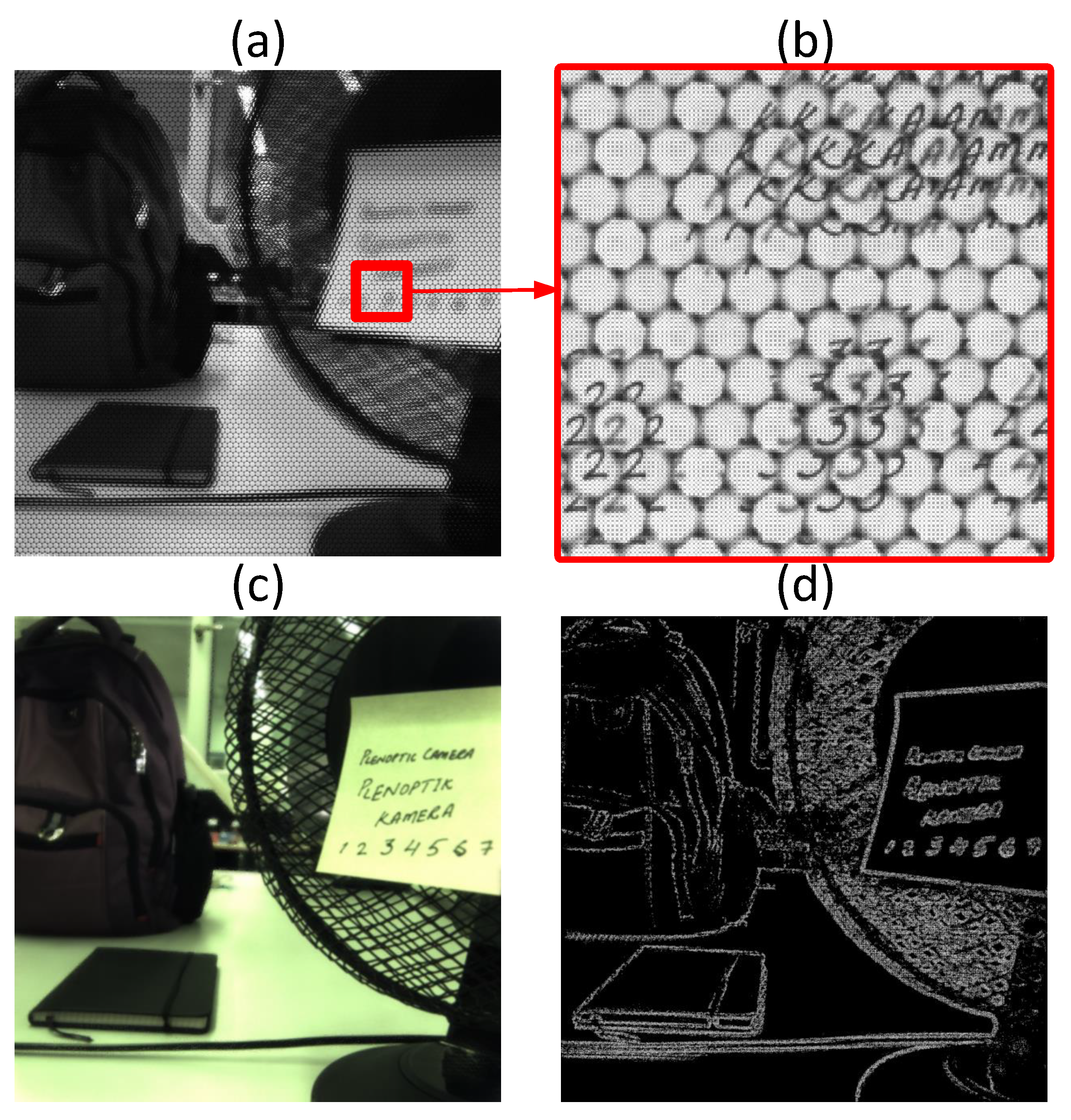
Figure 2.
(a) Raw image captured by plenoptic camera (b) part of the image displaying micro-images (c) resulting image after applying refocusing (d) estimated sparse depth map of the scene.
Figure 2.
(a) Raw image captured by plenoptic camera (b) part of the image displaying micro-images (c) resulting image after applying refocusing (d) estimated sparse depth map of the scene.

Figure 3.
Plenoptic camera model with two micro-lenses and corresponding planes.

Figure 4.
UML activity diagram of the modified depth estimation algorithm.

Figure 5.
Micro-lenses hexagonal arrangement in the MLA.

Figure 6.
Two adjacent micro-lenses in an MLA with center points and a reference point .

Figure 7.
Two parallel micro-images depicting the epipolar geometry of the stereo pair.

Figure 8.
UML structure diagram showing the dependencies between different components of the algorithm.
Figure 8.
UML structure diagram showing the dependencies between different components of the algorithm.

Figure 9.
Micro-images grid including reference and target micro-images placed at different baseline distances.
Figure 9.
Micro-images grid including reference and target micro-images placed at different baseline distances.

Figure 10.
Selection process of target micro-images entailing temporal parallelism.

Figure 11.
Stereo-matching between reference and target micro-images.

Figure 12.
Spatial parallelization during stereo-matching.

Figure 13.
Census transform with a reference pixel.

Figure 14.
Optimized hardware implementation with arbitrary width adders.

Figure 15.
Partitioned memory to ensure contiguous access. (a) Non-Contiguous (b) Contiguous.

Figure 16.
Circular shift-buffer for the algorithm.

Figure 17.
Xilinx Zynq UltraScale+ based hardware design for the plenoptic camera system.

Figure 18.
Raw image (left), filtered RxLive sparse depth map (middle) and filtered sparse depth map calculated by the presented algorithm (right).
Figure 18.
Raw image (left), filtered RxLive sparse depth map (middle) and filtered sparse depth map calculated by the presented algorithm (right).


Table 1.
Selected from sub-modules of the algorithm.
| Sub-Module | Description | |
|---|---|---|
| Pre-Processing | Consists of recursive operations to calculate the grid lines of micro-lens array, such as lens-type. | |
| Arranges and assigns the calculated micro-lens grid data to the corresponding micro-lenses. | ||
| Census Transform | Recursive operations to convert the input image to the transformed image with respect to the window size. | |
| Best-Match Computation | Selects reference micro-image and fetches the respective input data to find the correspondence. | |
| Recursive operations to select the target micro-images for matching. | ||
| Iterative search process to calculate error to find the correspondence across the target micro-image. | ||
| Depth-Evaluation | Transferring the calculated depth estimations to the memory. |
Table 2.
Sparse depth map images statistics.
| Std. Deviation | Density | Valid Pixels | ||
|---|---|---|---|---|
| chair | Presented Alg. | 0.161 | 0.842 | 882,533 |
| Zeller et al. [6] | 0.178 | 0.64 | 676,763 | |
| RxLive | 0.124 | 0.016 | 16,851 | |
| cup | Presented Alg. | 0.181 | 0.501 | 525,385 |
| Zeller et al. [6] | 0.173 | 0.413 | 433,148 | |
| RxLive | 0.160 | 0.072 | 75,108 |
Table 3.
Actual execution time, gain, utilization and error comparison.
| Optimization | Execution Time in ms | Gain in ms | Max. Latency in Clocks | BPR in % | Abs. Rel Error | Utilization Vivado | |||
|---|---|---|---|---|---|---|---|---|---|
| LUTs | FFs | BRAMs | DSPs | ||||||
| ,, | 1121.25 | 3.64 × 10⁹ | 18.36 | 0.146 | 15,628 | 19,623 | 10 | 16 | |
| , Temporal | 726.96 | 394.28 | 1.34 × 10⁹ | 18.36 | 0.146 | 16,986 | 20,520 | 10 | 16 |
| , Temporal | 604.06 | 122.89 | 1.85 × 10⁹ | 18.36 | 0.146 | 14,845 | 19,094 | 10 | 15 |
| , Spatial | 600.33 | 3.73 | 1.85 × 10⁹ | 18.36 | 0.146 | 18,291 | 21,619 | 10 | 40 |
| , Spatial | 562.62 | 37.71 | 2.08 × 10⁸ | 18.54 | 0.145 | 18,896 | 21,811 | 5 | 16 |
| Combination | 334.41 | 228.21 | 1.41 × 10⁷ | 18.36 | 0.146 | 20,900 | 25,150 | 5 | 13 |
| Hamm_Distance | 311.11 | 23.3 | 1.41 × 10⁷ | 18.37 | 0.146 | 21,446 | 25,085 | 10 | 267 |
| Memory_Opt. | 27.18 | 283.92 | 6.72 × 10⁶ | 18.45 | 0.147 | 29,412 | 28,769 | 1797 | 272 |
Table 4.
PC-system, mobile GPU and FPGA specifications.
| Platform | Specifications |
|---|---|
| PC-system | Corsair 200R desktop, Windows 10, Intel core i7-7700K CPU, 512 GB SSD and 16 GB RAM. |
| Mobile GPU | NVIDIA® Jetson Xavier NXTM, CUDA cores = 384, Max. Memory = 8 GB LPDDR4x @51.2 GBits/s. |
| FPGA MPSoC | Xilinx Zynq UltraScale + ZCU102 MPSoC contains LUTs = 274,080, FFs = 548,160 and BRAMs = 1824. |
Table 5.
PC-system, mobile GPU and FPGA comparison.
| Exec. Time per Frame | Throughput in fps | Power in W | Performance in fps/W | |
|---|---|---|---|---|
| PC-System | 88 ms | 11 | 85.1 | 0.13 |
| Mobile GPU | 34 ms | 29 | 13.4 | 2.19 |
| FPGA MPSoC | 27 ms | 37 | 7.1 | 5.21 |
Publisher’s Note: MDPI stays neutral with regard to jurisdictional claims in published maps and institutional affiliations. |
© 2021 by the authors. Licensee MDPI, Basel, Switzerland. This article is an open access article distributed under the terms and conditions of the Creative Commons Attribution (CC BY) license (https://creativecommons.org/licenses/by/4.0/).
Share and Cite
MDPI and ACS Style
Bhatti, F.; Greiner, T. Design of an FPGA Hardware Optimizing the Performance and Power Consumption of a Plenoptic Camera Depth Estimation Algorithm. Algorithms 2021, 14, 215. https://0-doi-org.brum.beds.ac.uk/10.3390/a14070215
AMA Style
Bhatti F, Greiner T. Design of an FPGA Hardware Optimizing the Performance and Power Consumption of a Plenoptic Camera Depth Estimation Algorithm. Algorithms. 2021; 14(7):215. https://0-doi-org.brum.beds.ac.uk/10.3390/a14070215
Chicago/Turabian StyleBhatti, Faraz, and Thomas Greiner. 2021. "Design of an FPGA Hardware Optimizing the Performance and Power Consumption of a Plenoptic Camera Depth Estimation Algorithm" Algorithms 14, no. 7: 215. https://0-doi-org.brum.beds.ac.uk/10.3390/a14070215
Note that from the first issue of 2016, this journal uses article numbers instead of page numbers. See further details here.