
A Hybrid Exact–Local Search Approach for One-Machine Scheduling with Time-Dependent Capacity
by
 ,
,
Christos Valouxis
1,
Christos Gogos
2,*,
Angelos Dimitsas
2,
Petros Potikas
3 and
Anastasios Vittas
2 1
Department of Electrical and Computer Engineering, University of Patras, 26500 Patras, Greece
2
Department of Informatics and Telecommunications, University of Ioannina, 47100 Arta, Greece
3
Department of Electrical and Computer Engineering, National Technical University of Athens, 15772 Athens, Greece
*
Author to whom correspondence should be addressed.
Algorithms 2022, 15(12), 450; https://0-doi-org.brum.beds.ac.uk/10.3390/a15120450
Submission received: 25 October 2022
/
Revised: 22 November 2022
/
Accepted: 25 November 2022
/
Published: 29 November 2022
(This article belongs to the Special Issue Scheduling: Algorithms and Applications)
Abstract
:Machine scheduling is a hard combinatorial problem having many manifestations in real life. Due to the schedule followed, the possibility of installations of machines operating sub-optimally is high. In this work, we examine the problem of a single machine with time-dependent capacity that performs jobs of deterministic durations, while for each job, its due time is known in advance. The objective is to minimize the aggregated tardiness in all tasks. The problem was motivated by the need to schedule charging times of electric vehicles effectively. We formulate an integer programming model that clearly describes the problem and a constraint programming model capable of effectively solving it. Due to the usage of interval variables, global constraints, a powerful constraint programming solver, and a heuristic we have identified, which we call the “due times rule”, the constraint programming model can reach excellent solutions. Furthermore, we employ a hybrid approach that exploits three local search improvement procedures in a schema where the constraint programming part of the solver plays a central role. These improvement procedures exhaustively enumerate portions of the search space by exchanging consecutive jobs with a single job of the same duration, moving cost-incurring jobs to earlier times in a consecutive sequence of jobs or even exploiting periods where capacity is not fully utilized to rearrange jobs. On the other hand, subproblems are given to the exact constraint programming solver, allowing freedom of movement only to certain parts of the schedule, either in vertical ribbons of the time axis or in groups of consecutive sequences of jobs. Experiments on publicly available data show that our approach is highly competitive and achieves the new best results in many problem instances.
1. Introduction
Scheduling problems are interesting due to their practical usefulness and hardness. Such problems emerge in various domains, including manufacturing, computing, project management, and many others. Since scheduling problems are typically NP-hard, several approaches compete to attain the often unreached optimal solutions. Metaheuristics, heuristics, constraint programming, and mathematical programming often yield excellent results. The latter two are especially sensitive to problem sizes since their exact nature implies that all solutions must be checked or intelligently pruned.
Scheduling is a thoroughly studied subject that is considered a discipline on its own [1]. Scheduling problems are classified using the commonly accepted notation [2], where refers to the machine environment, refers to the constraints, and refers to the objective function. A valuable asset for appreciating the variety of scheduling problems under the notation can be found at [3].
In this work, we study a variation in the one-machine scheduling with time-dependent capacity problem that Mencia et al. introduced in [4,5,6]. The problem emerged in the context of scheduling charge times for a fleet of electric vehicles and is an abstraction of the real problem. It is classified as , meaning that it involves a single machine with capacity that fluctuates through time, with no other constraints, and the objective is minimizing the accumulated tardiness from all jobs. The problem piqued our interest due to its precise definition, the publicly available datasets, and the excellent results that were already published and which we used for comparisons.
We propose a novel way to approach the problem based on a model with an embedded rule (the due times rule) that helps constraint programming solvers reach good solutions fast. We also propose three improvement procedures that are local search routines. We combine the exact and local search parts in our approach to the problem, and we manage to achieve results equal to or better than the best-known results for 91 and 48 cases, respectively, out of 190 public problem instances.
2. Problem Description
A detailed description of the problem exists in [6], so we give a brief description in this section. The problem involves n jobs and one machine with a certain capacity that varies over time. Each job i has a duration and a due date . All jobs are available from the start time () and consume one unit of the machine’s capacity for the period in which the job will eventually be scheduled. Once a job starts, it cannot be preempted and should continue execution until completion. It is imperative that the capacity of the machine is not exceeded at any time. Finally, the objective that should be minimized is the total tardiness of all jobs, which is computed based on the due dates of the jobs. If job i completes execution before its due date, it does not affect the cost. Otherwise, it imposes a cost equal to , where is the completion time that job i assumes in the schedule. The mathematical formulation of the problem is presented in Section 7.
The problem is NP-hard, since problems and (P denotes a known number of identical machines), which are known to be NP-hard [7], can be reduced to it.
Terminology
In line with the definitions of terms in [6], we use , , , and for the start time, duration, due time, and completion time, respectively, of a job i in a given schedule. Then, is the tardiness of job i which is .
A concrete example involving 12 jobs and a capacity line that reaches a maximum of four units is presented below. This example is the one used as Example 1 in [5]. Table 1 summarizes information related to it alongside the values associated with an optimal schedule for this problem instance, achieving an optimal cost of 20. The schedule corresponding to the table’s third line is presented graphically in Figure 1.
3. Dataset
A dataset consisting of a relatively large number of artificially generated problem instances is publicly available in [8]. The procedure for generating these instances is described in [6], and special care has been taken so that the problems’ structures resemble the structure manifested during the process of electric vehicle charging [9]. In total, 190 problem instances exist, as seen in Table 2. The naming of each problem instance is i<n>_<MC>_<k>, where n is the number of jobs, MC is the maximum capacity, and k is the sequence number of each problem instance for this n, MC pair.
Note that the capacity in all problem instances is a unimodal step function that grows until reaching a peak, then decreases, and finally stabilizes at a positive value.
4. Related Work
Hard combinatorial optimization problems, such as the one-machine scheduling with time-dependent capacity problem, are approached using numerous solving methods [10,11]. The two basic categories of such approaches are the exact ones and the heuristic–metaheuristic ones. In the first category, one can identify mathematical programming (i.e., linear programming, integer programming, and others) [12], constraint programming [13], approaches based on SAT (satisfiability) [14] or SMT (satisfiability modulo theory) solvers [15], and, in general, methods that intelligently examine the complete search space while pruning parts of it during their quest for proven optimal solutions [16]. In the second category, the approaches are numerous, including local search methods [17,18], genetic algorithms [19], genetic programming [20], memetic algorithms [21], differential evolution [22], ant colony optimization [23], particle swarm optimization [24], bees algorithms [25], hyper-heuristics [20], and others.
Heuristically Constructed Schedules
In [6], the authors present the schedule builder algorithm, where jobs are ordered in an arbitrary sequence, and each job is scheduled to start at the earliest possible time. After positioning each job, the capacity of the machine is updated in accordance with the partial schedule. When all jobs are scheduled, the algorithm finishes and returns a feasible schedule. This search space is guaranteed to contain an optimal solution to any problem instance [5]. So, each possible solution can be represented as a sequence of jobs to the schedule builder. Certain metaheuristic algorithms, such as genetic algorithms, may benefit from the idea of representing each possible schedule as a sequence of jobs and searching through the space of all possible permutations.
Here, we present in Algorithm 1 a modification to the schedule builder algorithm that introduces lanes, which are levels formed by the capacity of the problem. So, for example, a problem with a maximum capacity of four has four lanes; the first is always available during the time horizon, and the three others, based on the capacity, have periods of availability and unavailability. Lanes help plot schedules, disambiguate solutions with identical costs, and quickly identify jobs that form sequences of consecutive jobs. In Algorithm 1, we call the function find_lowest_available_lane that finds the lowest available lane that can accommodate a job starting at period t.
| Algorithm 1 Schedule builder using lanes |
|
5. C-Paths
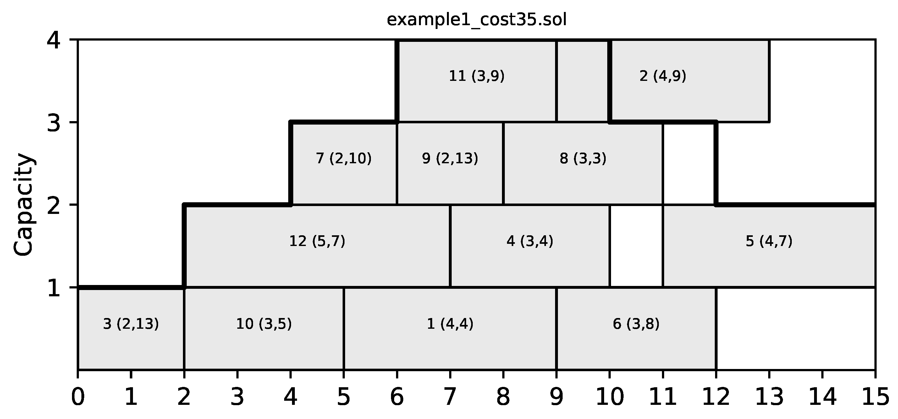
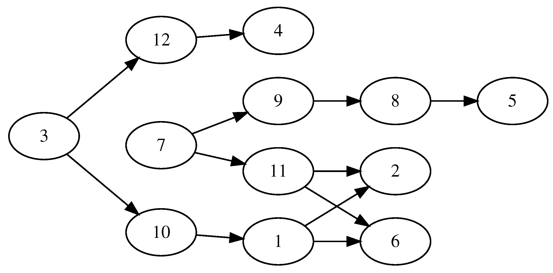
A fundamental concept that was introduced by Mencia et al. in [4] is the concept of a C-Path. A C-Path is a sequence of consecutive jobs (i.e., in a C-Path, the finish time of each previous job coincides with the start time of the following job) in a schedule. The importance of C-Paths stems from the fact that jobs in each C-Path can easily swap places and keep the schedule feasible. We can consider a graph view of a schedule, where each job is a node and directed edges connect nodes that correspond to consecutive jobs. Then, each path from a source node of the graph (i.e., a node with no incoming edges) to a sink node (i.e., a node with no outgoing edges) is a C-Path. This is demonstrated in Figure 2 for a sample schedule of cost 35 for the toy problem instance shown in Table 1 and its corresponding graph in Figure 3. The list of C-Paths identified in this graph includes the following six: (3,12,4), (3,10,1,6), (3,10,1,2), (7,9,8,5), (7,11,2), and (7,11,6).
The number of C-Paths might be very large, especially for schedules of big-size problems. This is demonstrated in Table 3, which shows the number of C-Paths for specific schedules of selected problem instances. Note that the number of C-Paths might change dramatically for different schedules of the same problem instance and that larger problem instances might have fewer C-Paths than smaller problem instances for some schedules.
Fast Computation of C-Paths
Since complete enumeration of all C-Paths is out of the question for problems of large sizes, we opted for a faster method of generating a single C-Path each time it is needed. This method starts by picking a random job, followed by two processes that find the right and the left part of a C-Path, having the selected job as a pivot element. The right-side part of the C-path is formed by choosing the next job that starts at the finish time of the current job. If more than one job exists, one of them is randomly selected and becomes the new current job. This process continues until no more subsequent jobs are found. The left side of the C-Path is formed by setting the initially selected job as the current job once again and finding previous jobs that end at the start time of the current job. Similarly, if more than one exists, one is chosen at random and becomes the new current job. The process ends when no more suitable prior jobs can be found.
6. Due Times Rule
This work contributes to identifying a rule that involves the due times of jobs with equal durations. The rule states that “Jobs with equal duration should be scheduled in the order of their due times”. In other words, if two jobs have equal durations, they should swap places if the due time of the job that is scheduled later is sooner than the due time of the job that is scheduled sooner. This rule can be used to strengthen mathematical formulations or as a heuristic for reaching better solutions.
Proof.
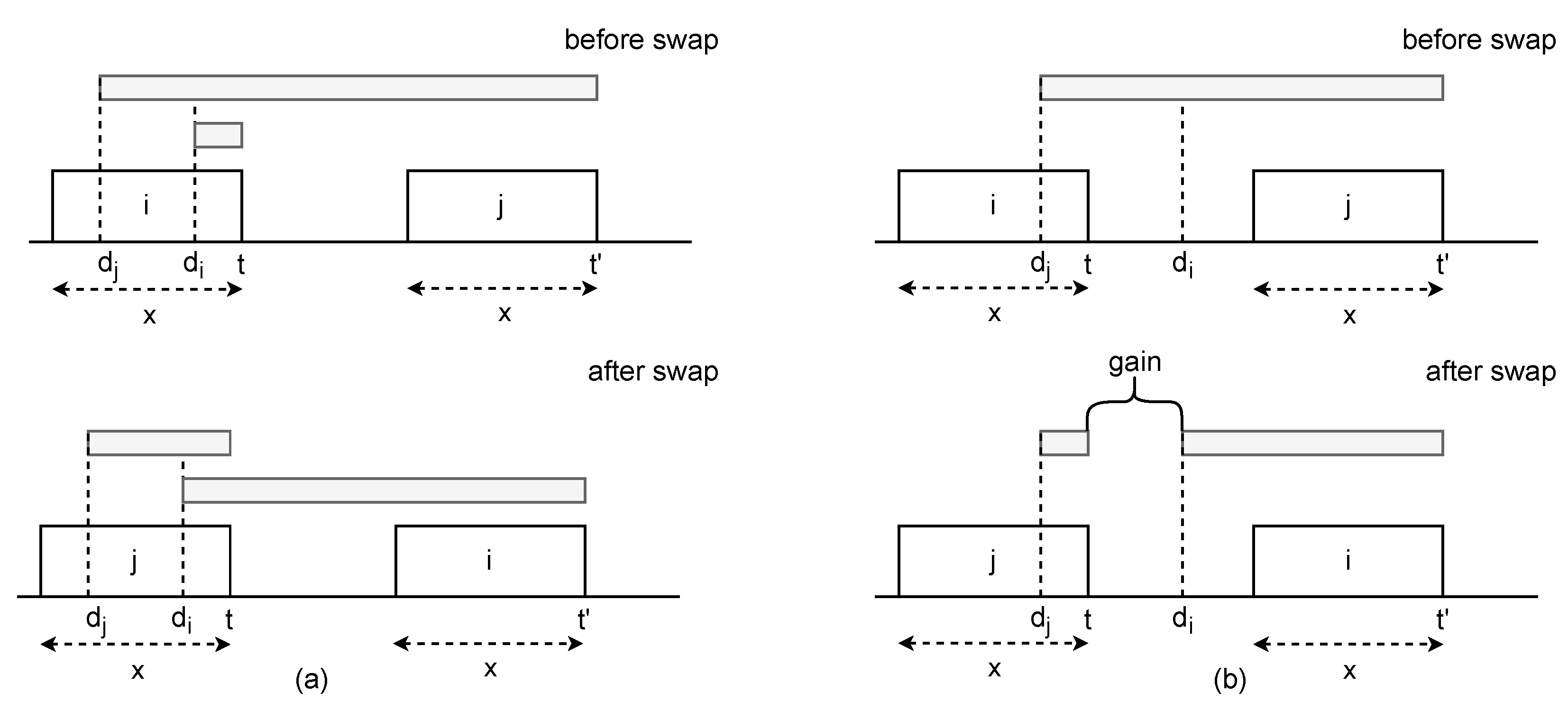
Suppose that two jobs, i and j, with the same duration, are scheduled such that job i comes first and job j follows. Additionally, suppose that job j has an earlier due time than job i, i.e., . Let t and be the finish times of jobs i and j, respectively, and since both jobs have the same duration, holds. When both jobs have non-negative tardiness values, i.e., and , swapping the jobs results again in non-negative tardiness values for both jobs. This holds because the tardiness of job j after the swap will be . Moreover, , so the tardiness of job i after the swap will be . So, the total tardiness before the swap is , which is equal to the total tardiness after the swap, which is . This situation is depicted in Figure 4a. The top figure shows a possible configuration of two equal-duration jobs that both incur tardiness. It can be easily seen that the total length of the gray bars that represent the tardiness remains the same after swapping jobs i and j.
The benefit of positioning equal-duration jobs according to their due times occurs when job i completes execution before its due time, and job j incurs some positive value of tardiness. Since job i has no tardiness, the total tardiness of the initial configuration is . After the swap, the total tardiness will be . In order to prove that the total tardiness is no greater after the swap, the following inequality must hold: . This inequality leads to the following true proposition: . The last inequality holds since it is the assumption made for this case, i.e., job i has no tardiness. A visual representation of such a situation is depicted in Figure 4b. The upper part of the figure shows the situation where job i is scheduled first, while the lower part of the figure shows the situation after swapping the jobs. Again, the gray bars represent the tardiness of the jobs, and it can be seen that the total tardiness is decreased when the jobs swap places. □
7. Formulation and Implementation
A formulation of the problem that will be used to construct initial solutions to the problem is presented below. Then, the formulation is slightly modified and used for solving problems involving subsets of tasks in an effort to attain better schedules overall.
Let be the set of jobs.
Let be the duration of each job .
Let be the due date of each job .
Let T be the number of time points. Note that the value of T is not given explicitly by the problem, but such a value can be computed by aggregating the duration of all jobs.
Let be the capacity of the machine at each time point .
We define integer decision variables that denote the start time of each job .
Likewise, we define integer decision variables that denote the finish time of each job .
We also define integer decision variables which denote the tardiness of each job .
Finally, we define binary decision variables and . Each one of the former variables assumes the value 1 if job j starts its execution at time point t, or else it assumes the value 0. Likewise, each variable marks the time point at which job j finishes.
A brief explanation of the above model follows.
The aim of the objective function in Equation (1) is to minimize the total tardiness of all jobs.
Equation (2) assigns the proper finish time value to each job given its start time and duration.
Equation (3) assigns tardiness values to the jobs. In particular, when job j finishes before its due time, the right side of the inequality is a negative number, and variable assumes the value 0 since its domain is non-negative integers. When job j finishes after its due time, becomes . This occurs because is included in the minimized objective function and therefore forced to assume the smallest possible non-negative value.
Equations (4) and (5) drive the variables to proper values based on the values. This occurs because, when assumes the value t, becomes 1. It should be noted that M in Equation (5) represents a big value, and can be used for it. For the specific time point t at which a job will be scheduled to begin, the right sides of both equalities will assume the value t. For all other time points besides t, the right sides of the former and the latter equations become 0 and M, respectively.
Equation (6) enforces that only one among all of the variables of each job j will assume the value 1.
Equation (7) dictates the following association rule: for each job j, when becomes 1 or 0, the corresponding y variable of j with the time offset , which is , will also be 1 or 0, respectively.
Equation (8) guarantees that for each time point, the capacity of the machine will not be violated. The values that the left side of the equation assumes are the numbers of active jobs at each time point t. The first double summation counts the jobs that have started no later than t, while the second double summation counts the jobs that have also finished no later than t. Their difference is obviously the number of active jobs.
Constraint Programming Formulation
The IBM ILOG constraint programming (CP) solver seems to be a good choice for solving scheduling problems involving jobs that occupy intervals of time and consume some types of resources that have time-varying availability [27]. The one-machine scheduling problem can be easily formulated in the IBM ILOG CP solver using one fixed-size interval variable per job (j) and the constraint always_in, which restricts all of them to assume values that collectively never exceed the maximum available capacity over time. This is possible by using a pulse cumulative function expression that represents the contribution of our fixed interval variables over time. Each job execution requires one capacity unit, which is occupied when the job starts, retained through its execution, and released when the job finishes. In our case, the variable usage aggregates all pulse requirements by all jobs. The objective function uses a set of integer variables z[job.id] that are stored in a dictionary that has the identifier of each job as keys. Each z[job.id] variable assumes the value of the job’s tardiness (i.e., the non-negative difference of the job’s due time (job.due_time) and its finish time (end_of(j[job.id])). An additional constraint is added that corresponds to the due times rule mentioned in Section 6. Jobs are grouped by duration, and a list ordered by due times is prepared for each group. Then, for all jobs in the list, the constraint enforces that the order of the jobs must be respected. This means that each job in the list should have an earlier start time than the start time of the job that follows it in the list. The model implementation using the IBM ILOG CP solver’s python API is presented below.
import docplex.cp.model as cpx
model = cpx.CpoModel()
x_ub = int(problem.ideal_duration() * 1.1)
j = {
job.id: model.interval_var(
start=[0, x_ub - job.duration - 1],
end=[job.duration, x_ub - 1],
size=job.duration
)
for job in problem.jobs
}
z = {
job.id: model.integer_var(lb=0, ub=x_ub - 1)
for job in problem.jobs
}
usage = sum([model.pulse(j[job.id], 1) for job in problem.jobs])
for i in range(problem.nint):
model.add(
model.always_in(
usage,
[problem.capacities[i].start, problem.capacities[i].end],
0,
problem.capacities[i].capacity,
)
)
for job in problem.jobs:
model.add(z[job.id] >= model.end_of(j[job.id]) - job.due_time)
for k in problem.size_jobs: # iterate over discrete job durations
jobs_by_due_time = same_duration_jobs[k]
for i in range(len(jobs_by_due_time)-1):
j1, j2 = jobs_by_due_time[i][1], jobs_by_due_time[i+1][1]
model.add(model.start_of(z[j1]) <= model.start_of(z[j2]))
model.minimize(sum([z[job.id] for job in problem.jobs]))
The object problem is supposed to be an instance of a class that has all relevant information for the problem instance under question (i.e., jobs is the list of all jobs, each job besides id and due_time has also a duration property, nint is the number of capacity intervals, and capacities[i].start and capacities[i].end are the start time and end time of the ith capacity step, respectively). Finally, the problem object has the ideal_duration method that estimates a tight value for the makespan of the schedule, which is incremented by 10% to accommodate possible gaps that hinder the full exploitation of the available capacity. The “ideal duration” is computed by totaling the durations of all jobs and then filling the area under the capacity line from left to right and from bottom to top with blocks of the size until the totaled durations quantity runs out. The rightmost point on the time axis of the filled area becomes the “ideal duration” and is clearly a relaxation of the actual completion time of the optimal solution since each job is decomposed in blocks of the duration one, and no gaps appear in the filled area.
An effort was undertaken to implement the above model using Google’s ORTools CP-SAT Solver [28]. This solver has a cumulative constraint that can be used in place of always_in to describe the machine’s varying capacity. A series of variables were used that transformed the pulse of the capacity to a flat line equal to the maximum capacity. Unfortunately, the solver under this specific model implementation could not approximate good results and was finally not used.
8. Local Search Improvement Procedures
We have identified three local search procedures that have the potential to improve the cost of a given schedule. These local search procedures can be considered as “large” moves since they examine a significant number of schedules neighboring the current one.
8.1. Local Search Improve1
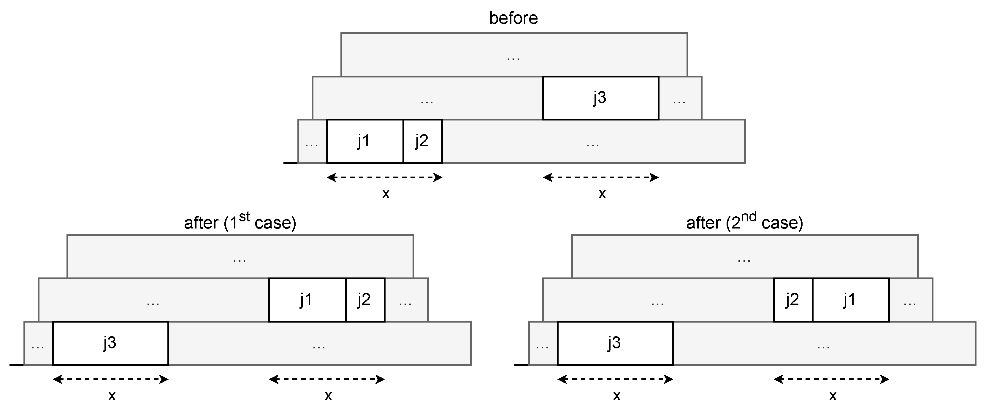
The first local search procedure starts by iterating overall jobs. For each job , each other consecutive job is identified, and then each job with a duration equal to the aggregated durations of and is found. Since and are consecutive, they can be swapped with job , and the schedule will still remain feasible, as seen in Figure 5. Moreover, the order of the two first jobs does not influence the feasibility. So, two alternatives are tested that compare the imposed penalties before and after the swap, and, if an improvement is found, the swap occurs. The time complexity of this procedure is since the maximum number of consecutive jobs for each job is bounded by the maximum capacity, which is a constant number much smaller than the number of jobs. Moreover, the identification of consecutive jobs and jobs of durations that are equal to the aggregated duration of two other consecutive jobs is performed using Hash Maps that effectively contribute to the above complexity. The first one uses times as keys and has a list of jobs starting at these times as values. By using as a key the finish time of a job , the dictionary returns each job that is consecutive to . The second Hash Map uses the jobs’ durations as keys and, as the value for each key x, the list of jobs with the duration x. Note that the second Hash Map is computed only once and remains unchanged through the solution process.
8.2. Local Search Improve2
The second local search procedure uses C-Paths that are computed as described in Section 5. Each C-Path is traversed from left to right until a job j is found that imposes a cost to the schedule (i.e., has a finish time greater than its due time). The only way that the penalty of a job j can be reduced is by moving it to the left side of the C-Path. So, all jobs that start earlier than job j are examined by swapping places with job j. If the total penalty imposed by job j and a sequence of jobs up to another job k is greater than the penalty after swapping jobs j and k, followed by shifts of jobs in between, then this set of moves occurs. The time complexity of this procedure is . Since each C-Path has a length that is , and each C-Path is traversed once for identifying jobs with penalties, and then, for each such job, the C-path is again traversed, it follows that the complexity is quadratic. The construction of each C-Path costs , which is added to the time of the above procedure and gives . Since this occurs for every job, C-Paths are generated, and this results in a total complexity of for the second local search procedure. An example of this procedure is depicted in Figure 6.
8.3. Local Search Improve3
The third local search procedure starts by identifying periods where the capacity is not fully used. Given a capacity profile that has the form of a pulse, for each job, the pulse is lowered by one unit for the period during which it is active. This is iterated for all jobs, and, finally, it is possible to exist periods scattered across the horizon that have non-zero capacity remaining. So, jobs with finish times that fall inside these periods (gaps) can possibly be moved to the right, and the schedule should still be feasible. The main idea of this local search procedure is that it allows two jobs of marginally different durations to swap places. This occurs by first identifying two C-Paths with no common jobs that have jobs with finish times falling inside gaps as their rightmost jobs. Given two such C-Paths, each job of them can be swapped with a job of the other C-Path, provided that the slack that the gap provides is adequate for this move. This means that all jobs of a C-Path that are to the right of the smaller of the two swapping jobs should shift to the right, and all jobs of the other C-Path that are to the right of the bigger job should shift to the left, giving the opportunity for further penalty gains. In principle, the number of jobs that might have finish times that fall inside gaps is , but our experiments showed that, in practice, this number is a small fraction of . Since two C-Paths are involved, and each job of a C-Path has to be checked with each job of the other C-Path, this contributes . Moreover, all possible pairs of jobs that fall in gaps are used as starting points in the construction of the corresponding C-Paths, resulting in another term. So, the time complexity of the overall procedure is . It should be noted that shifts due to penalty reductions occur rarely, and their amortized contribution to the time complexity is neglected. In practice, the time needed for this move is comparable to the previous one due to the relatively small number of jobs that fall inside gaps. An example of this procedure is depicted in Figure 7.
9. A Multi-Staged Approach
The approach we employed for addressing the problem uses several stages that operate cyclically until the available time runs out.
10. Results
Our experiments were run on a workstation with 32GB of RAM and an Intel Core i7-7700K 4.2GHz CPU (four cores, eight threads) running Windows 10. The constraint programming solver that we used was IBM ILOG CP Optimizer Version 22. The local search procedures, the implementation of the constraint programming model, and the driver program were all implemented in Python. Our results are compared with the results of Mencia et al. in [6], which is a continuation of their previous work in [4,5]. In their most recent work, they present and compare six memetic algorithms termed , , , , , and . The last one gives the best results out of all others and the previous approaches of the authors, and this is the algorithm with which we compare our approach. combines CB and ICP procedures under a memetic algorithm. Both procedures use the concept of a cover. A cover is a disjoint set of C-Paths that covers all jobs. In CB, once a cover is generated, the C-Paths of the cover are examined in isolation for improvements. On the other hand, ICP swaps jobs between C-Paths, again using a cover to select the C-Paths participating in the procedure. In [6], no values for the schedule costs are given, but the relative performances of the six approaches are recorded in tables and graphs instead. So, results about the actual schedule costs of and the other approaches that we use in our comparisons hereafter were taken from [8], which the authors cite in their paper.
10.1. CPO vs. CPO+
We call the constraint programming approach, briefly described in [6], CPO (constraint programming optimizer), and our approach described in Section “Constraint Programming Formulation” that exploits the “due rule”, CPO+. Results about the performance of CPO were taken from the web repository cited at the end of the previous paragraph.
Table 4 depicts for each problem instance the total tardiness of all jobs for the schedule that CPO and CPO+ produced. It shows that CPO+ manages to find solutions equal to the best-known solutions for 25 out of 190 problem instances, while CPO achieves this for only 2 problem instances (i120_3_3 and i120_5_4). The best values are written in bold. An allotted time of seconds for each problem instance was given for each run, where n is the number of jobs. We used all available cores, which was the default setup for the IBM ILOG CP Optimizer. The results of CPO+ are the best among 10 runs for each problem instance, and random seeds were used to achieve diversity.
10.2. Hybrid Exact–Local Search
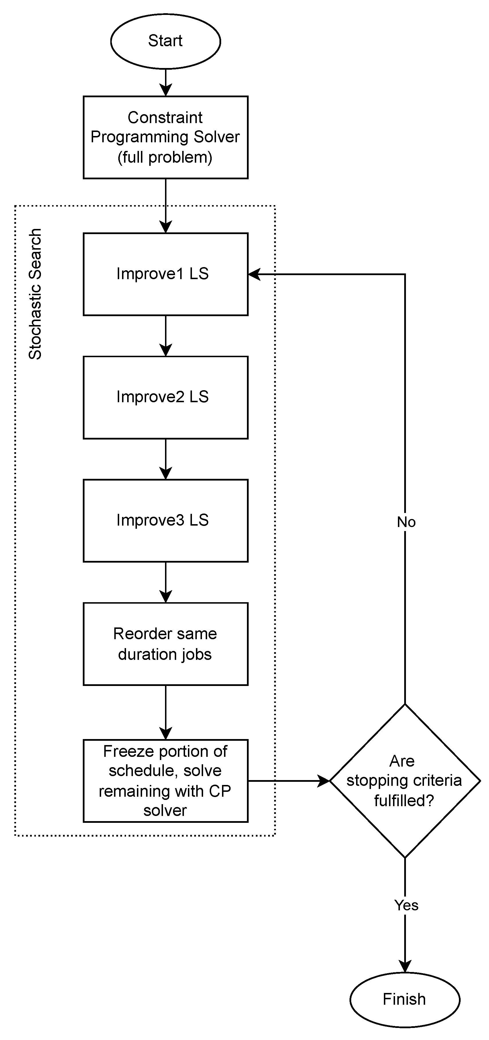
The HELS (hybrid exact–local search) approach is shown using the flowchart in Figure 8. First, the constraint programming solver is employed for the full problem. A period of time of seconds is given for executing this stage. Then, for seconds, a loop occurs that includes the three local search procedures, followed by activation of the constraint programming solver again, but this time for subproblems. These subproblems might involve jobs that intersect with vertical ribbons on the time axis or groups of consecutive sequences of jobs (i.e., multiple C-Paths). Note that a reordering of jobs might be needed so that the current solution conforms with the “due rule”, else the constraint programming solver might consider the fixed parts of the partial solution to be infeasible. This is denoted by the extra stage “Reorder same duration jobs” after the third local search procedure in Figure 8.
Table 5 presents the best results that were achieved by the approach with the best-known results, all of which are provided by .
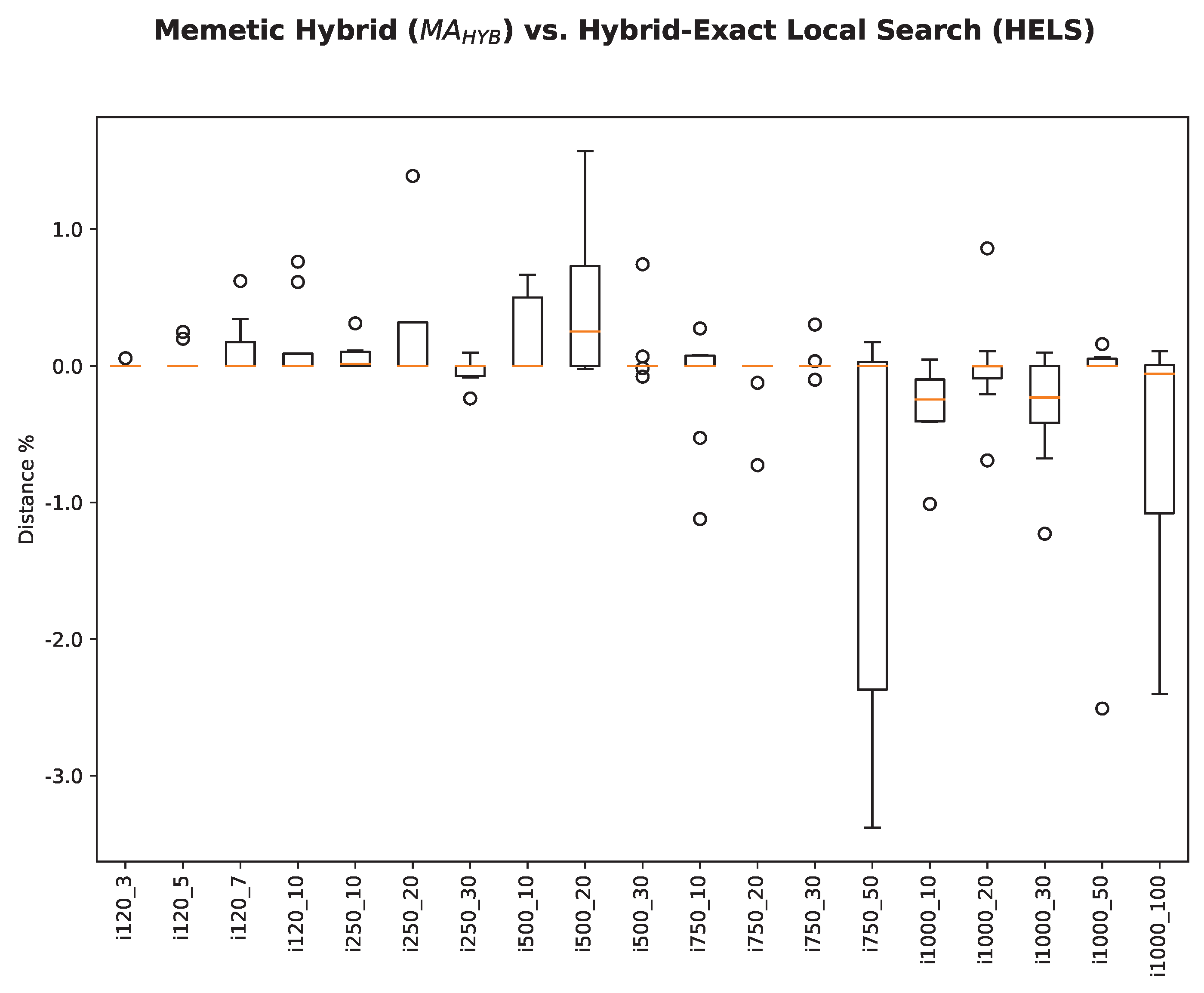
Table 6 consolidates the relative performance of our approach when compared with the best-known results. We can observe that our approach manages to find new best results for 48 of the problem instances. It also equals the best-known results for 91 problem instances. achieves better results than our approach for the remaining 51 problem instances. We also compare our solutions with how closely it reaches the previously best-known solution as a percentage value, and we call this the metric “distance%”. Negative values mean that our approach sets a new best-known value. We see that the average distance% metric for all problem instances assumes a negative value of , demonstrating its very good performance. This is further supported by Figure 9, which shows for each problem subset consisting of 10 instances, a boxplot of the distance% values. Again, negative values are advantageous for our approach, and the graph clearly shows that our approach achieves excellent results, especially for large problem instances.
10.3. Discussion
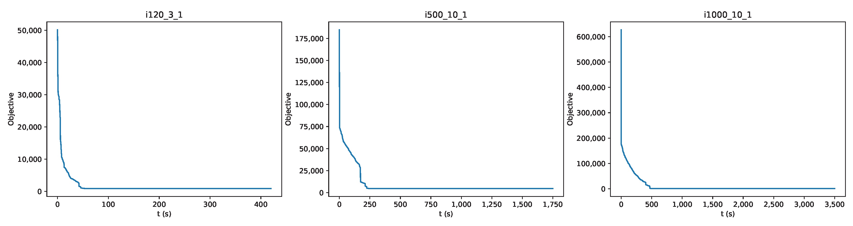
Figure 10 includes three graphs showing the cost of solutions during the allotted execution time. We can see that the costs start from very high values and sharply fall to smaller values, not very far from the final ones. The long tails of the graphs indicate that less time is needed for achieving good quality schedules than the seconds (n is the number of jobs) that we have used in our experiments. This is further demonstrated by the values of CPO+ and HELS in Table 4 and Table 5, with the first ones being close to the second. In particular, for the set of all 190 problem instances, the percentage distance of CPO+ to HELS has a mean equal to 0.077 and a standard deviation equal to 0.069.
Regarding comparing our approach with the one by Mencia et al. [6], we can make a few remarks. First, Mencia et al. do not report in their papers the exact values that their approaches returned; instead, they compare their results to their other less efficient approaches. So, we retrieved the values we use in our comparisons from the site [8] that the authors reference in their paper. Providing exact values alongside solution files that other researchers can download from our repository [26] may attract more interest to the problem. Since the run-time environments used in our case and in Mencia et al.’s case are different, we focus mainly on whether each approach can find the best possible result, given that limited processing power is exploited in both cases. Furthermore, in our case, Figure 10 clearly shows a trend observed in other problem instances: our approach reaches results very close to the final results using only about of the allotted execution time.
11. Conclusions
In this manuscript, we examined an abstraction of a real-world electrical vehicle charging scheduling problem that comes with a public dataset and high-quality published solutions. This problem involves a number of jobs with given durations and due times that should be scheduled to a single machine with time-dependent capacity, while the objective is the minimization of the aggregated tardiness of all jobs. We proposed some novel ideas, such as the due times rule, local improvement procedures, and problem decompositions. The result was that we managed to achieve better solutions for many problem instances of the already excellent solved dataset. A central component of the proposed approach, which we call the hybrid exact–local search (HELS) approach, is a constraint programming model that utilizes interval variables and global constraints and that is initially called for the full problem and then iteratively for subproblems that stochastically drive the objective to more favorable values. Three improvement procedures are embedded in our HELS approach that perform local searches and succeed in further improving solutions. Our work demonstrates an example of a general tendency. Challenging combinatorial problems increasingly fall into the realm of exact solvers, which are nowadays capable of solving problems of big sizes. If this is not possible for the full problem, hybrid approaches that combine exact solvers over subproblems and approximate solvers can be combined to decompose the problem in a process that results in complete, high-quality solutions.
Author Contributions
Conceptualization, C.G. and C.V.; methodology, C.V.; software, C.G., C.V., and A.D.; validation, C.V., A.D., and P.P.; formal analysis, P.P.; investigation, A.D. and C.G.; resources, A.V.; data curation, A.V.; writing—original draft preparation, A.D. and C.G.; writing—review and editing, C.G., C.V., and A.D.; visualization, A.V.; supervision, C.G. All authors have read and agreed to the published version of the manuscript.
Funding
This research received no external funding.
Data Availability Statement
Problem instances and all solution files using our hybrid exact–local search approach are archived in [26].
Conflicts of Interest
The authors declare no conflict of interest.
References
- Pinedo, M.L. Scheduling; Springer: Berlin/Heidelberg, Germany, 2012; Volume 29. [Google Scholar]
- Graham, R.L.; Lawler, E.L.; Lenstra, J.K.; Kan, A.R. Optimization and approximation in deterministic sequencing and scheduling: A survey. In Annals of Discrete Mathematics; Elsevier: Amsterdam, The Netherlands, 1979; Volume 5, pp. 287–326. [Google Scholar]
- Scheduling Zoo. Available online: http://schedulingzoo.lip6.fr/ (accessed on 21 November 2022).
- Mencía, C.; Sierra, M.R.; Mencía, R.; Varela, R. Genetic algorithm for scheduling charging times of electric vehicles subject to time dependent power availability. In Proceedings of the International Work-Conference on the Interplay between Natural and Artificial Computation, Corunna, Spain, 19–23 June 2017; Springer: Berlin/Heidelberg, Germany, 2017; pp. 160–169. [Google Scholar]
- Mencía, C.; Sierra, M.R.; Mencía, R.; Varela, R. Evolutionary one-machine scheduling in the context of electric vehicles charging. Integr.-Comput.-Aided Eng. 2019, 26, 49–63. [Google Scholar] [CrossRef]
- Mencía, R.; Mencía, C. One-Machine Scheduling with Time-Dependent Capacity via Efficient Memetic Algorithms. Mathematics 2021, 9, 3030. [Google Scholar] [CrossRef]
- Koulamas, C. The single-machine total tardiness scheduling problem: Review and extensions. Eur. J. Oper. Res. 2010, 202, 1–7. [Google Scholar] [CrossRef]
- GitHub Repository for “One Machine Scheduling with Time Dependent Capacity via Efficient Memetic Algorithms” by Mencia R. Available online: https://github.com/raulmencia/One-Machine-Scheduling-with-Time-Dependent-Capacity-via-Efficient-Memetic-Algorithms (accessed on 21 November 2022).
- Hernández-Arauzo, A.; Puente, J.; Varela, R.; Sedano, J. Electric vehicle charging under power and balance constraints as dynamic scheduling. Comput. Ind. Eng. 2015, 85, 306–315. [Google Scholar] [CrossRef] [Green Version]
- Lenstra, J.K.; Kan, A.R.; Brucker, P. Complexity of machine scheduling problems. In Annals of Discrete Mathematics; Elsevier: Amsterdam, The Netherlands, 1977; Volume 1, pp. 343–362. [Google Scholar]
- Gupta, S.K.; Kyparisis, J. Single machine scheduling research. Omega 1987, 15, 207–227. [Google Scholar] [CrossRef]
- Gogos, C.; Valouxis, C.; Alefragis, P.; Goulas, G.; Voros, N.; Housos, E. Scheduling independent tasks on heterogeneous processors using heuristics and Column Pricing. Future Gener. Comput. Syst. 2016, 60, 48–66. [Google Scholar] [CrossRef]
- Baptiste, P.; Le Pape, C.; Nuijten, W. Constraint-Based Scheduling: Applying Constraint Programming to Scheduling Problems; Springer Science & Business Media: Berlin/Heidelberg, Germany, 2001; Volume 39. [Google Scholar]
- Großmann, P.; Hölldobler, S.; Manthey, N.; Nachtigall, K.; Opitz, J.; Steinke, P. Solving periodic event scheduling problems with SAT. In Proceedings of the International Conference on Industrial, Engineering and other Applications of Applied Intelligent Systems, Dalian, China, 9–12 June 2012; Springer: Berlin/Heidelberg, Germany, 2012; pp. 166–175. [Google Scholar]
- Ansótegui, C.; Bofill, M.; Palahí, M.; Suy, J.; Villaret, M. Satisfiability modulo theories: An efficient approach for the resource-constrained project scheduling problem. In Proceedings of the Ninth Symposium of Abstraction, Reformulation, and Approximation, Parador de Cardona, Spain, 17–18 July 2011. [Google Scholar]
- Brucker, P.; Knust, S.; Schoo, A.; Thiele, O. A branch and bound algorithm for the resource-constrained project scheduling problem. Eur. J. Oper. Res. 1998, 107, 272–288. [Google Scholar] [CrossRef]
- Vaessens, R.J.M.; Aarts, E.H.; Lenstra, J.K. Job shop scheduling by local search. Informs J. Comput. 1996, 8, 302–317. [Google Scholar] [CrossRef] [Green Version]
- Matsuo, H.; Juck Suh, C.; Sullivan, R.S. A controlled search simulated annealing method for the single machine weighted tardiness problem. Ann. Oper. Res. 1989, 21, 85–108. [Google Scholar] [CrossRef]
- Lee, K.M.; Yamakawa, T.; Lee, K.M. A genetic algorithm for general machine scheduling problems. In Proceedings of the 1998 Second International Conference Knowledge-Based Intelligent Electronic Systems, Proceedings KES’98 (Cat. No. 98EX111), Adelaide, Australia, 21–23 April 1998; IEEE: Piscataway, NJ, USA, 1998; Volume 2, pp. 60–66. [Google Scholar]
- Gil-Gala, F.J.; Mencía, C.; Sierra, M.R.; Varela, R. Evolving priority rules for on-line scheduling of jobs on a single machine with variable capacity over time. Appl. Soft Comput. 2019, 85, 105782. [Google Scholar] [CrossRef]
- França, P.M.; Mendes, A.; Moscato, P. A memetic algorithm for the total tardiness single machine scheduling problem. Eur. J. Oper. Res. 2001, 132, 224–242. [Google Scholar] [CrossRef]
- Wu, X.; Che, A. A memetic differential evolution algorithm for energy-efficient parallel machine scheduling. Omega 2019, 82, 155–165. [Google Scholar] [CrossRef]
- Merkle, D.; Middendorf, M. Ant colony optimization with global pheromone evaluation for scheduling a single machine. Appl. Intell. 2003, 18, 105–111. [Google Scholar] [CrossRef]
- Lin, T.L.; Horng, S.J.; Kao, T.W.; Chen, Y.H.; Run, R.S.; Chen, R.J.; Lai, J.L.; Kuo, I.H. An efficient job-shop scheduling algorithm based on particle swarm optimization. Expert Syst. Appl. 2010, 37, 2629–2636. [Google Scholar] [CrossRef]
- Yuce, B.; Fruggiero, F.; Packianather, M.S.; Pham, D.T.; Mastrocinque, E.; Lambiase, A.; Fera, M. Hybrid Genetic Bees Algorithm applied to single machine scheduling with earliness and tardiness penalties. Comput. Ind. Eng. 2017, 113, 842–858. [Google Scholar] [CrossRef]
- GitHub Repository for “A Hybrid Exact-Local Search Approach for One-Machine Scheduling with Time-Dependent Capacity” by Gogos C. Available online: https://github.com/chgogos/1MSTDC (accessed on 21 November 2022).
- Laborie, P.; Rogerie, J.; Shaw, P.; Vilím, P. IBM ILOG CP optimizer for scheduling. Constraints 2018, 23, 210–250. [Google Scholar] [CrossRef]
- Google OR Tools CP-SAT Solver. Available online: https://developers.google.com/optimization/cp/cp_solver (accessed on 21 November 2022).
Figure 1.
A graphical representation of the schedule in the last line of Table 1.
Figure 1.
A graphical representation of the schedule in the last line of Table 1.

Figure 2.
A suboptimal schedule of cost 35 for the toy problem of Table 2. Each job is depicted with a box and annotated with a label of the form , where x is the job identification number, y is the duration of the job, and z is its due time.
Figure 2.
A suboptimal schedule of cost 35 for the toy problem of Table 2. Each job is depicted with a box and annotated with a label of the form , where x is the job identification number, y is the duration of the job, and z is its due time.

Figure 3.
The graph that corresponds to the schedule of Figure 2.
Figure 3.
The graph that corresponds to the schedule of Figure 2.

Figure 4.
(a) Both job i and job j have non-negative tardiness values. (b) Job i has no tardiness, but job j incurs tardiness.
Figure 4.
(a) Both job i and job j have non-negative tardiness values. (b) Job i has no tardiness, but job j incurs tardiness.

Figure 5.
Assuming that job has the same duration as the aggregated duration of jobs and , two cases for swapping them become possible. The first one puts first and second, and the other one puts first and second.
Figure 5.
Assuming that job has the same duration as the aggregated duration of jobs and , two cases for swapping them become possible. The first one puts first and second, and the other one puts first and second.

Figure 6.
Given a C-Path, this local search procedure swaps two non-consecutive jobs ( and ) and appropriately shifts the in-between jobs () so as to keep the C-Path property for all involved jobs.
Figure 6.
Given a C-Path, this local search procedure swaps two non-consecutive jobs ( and ) and appropriately shifts the in-between jobs () so as to keep the C-Path property for all involved jobs.

Figure 7.
Jobs belonging to two C-Paths swap places to reduce the length or even remove gaps in the schedule.
Figure 7.
Jobs belonging to two C-Paths swap places to reduce the length or even remove gaps in the schedule.

Figure 8.
Hybrid Exact–Local Search approach.

Figure 9.
The HELS approach compared with the best-known results derived from the approach in [6].
Figure 9.
The HELS approach compared with the best-known results derived from the approach in [6].

Figure 10.
Cost values during the execution time using the HELS approach.


Table 1.
A sample problem instance with 12 jobs. For each job i, the table shows its duration and its due time . Additionally, for a certain schedule, the table shows the start time , completion time , and penalty incurred for each job i.
Table 1.
A sample problem instance with 12 jobs. For each job i, the table shows its duration and its due time . Additionally, for a certain schedule, the table shows the start time , completion time , and penalty incurred for each job i.
| i | 1 | 2 | 3 | 4 | 5 | 6 | 7 | 8 | 9 | 10 | 11 | 12 |
|---|---|---|---|---|---|---|---|---|---|---|---|---|
| 4,4 | 4,9 | 2,13 | 3,4 | 4,7 | 3,8 | 2,10 | 3,3 | 2,13 | 3,5 | 3,9 | 5,7 | |
| 4,8,4 | 8,12,3 | 10,12,0 | 2,5,1 | 6,10,3 | 5,8,0 | 8,10,0 | 0,3,0 | 12,14,1 | 3,6,1 | 6,9,0 | 9,14,7 |
Table 2.
Problem instances in the dataset. For each pair of a number of jobs and a maximum capacity, 10 individual problem instances exist.
Table 2.
Problem instances in the dataset. For each pair of a number of jobs and a maximum capacity, 10 individual problem instances exist.
| Number of Jobs (n) | Maximum Capacity (MC) |
|---|---|
| 120 | 3, 5, 7, 10 |
| 250 | 10, 20, 30 |
| 500 | 10, 20, 30 |
| 750 | 10, 20, 30, 50 |
| 1000 | 10, 20, 30, 50, 100 |
Table 3.
Number of C-Paths for schedules of selected problem instances, which can be found in [26].
Table 3.
Number of C-Paths for schedules of selected problem instances, which can be found in [26].
| Problem Instance | Schedule Cost | Number of C-Paths |
|---|---|---|
| i120_3_1 | 848 | 3 |
| i120_10_1 | 749 | 71 |
| i250_10_1 | 4094 | 48 |
| i250_30_1 | 3013 | 276 |
| i500_10_1 | 4614 | 204 |
| i500_30_1 | 2670 | 4528 |
| i750_10_1 | 4409 | 22,302 |
| i750_50_1 | 5134 | 206,022 |
| i1000_10_1 | 641 | 903,826 |
| i1000_100_1 | 71,012 | 216,694 |
Table 4.
Best results (total tardiness) from the CPO approach and our CPO+ approach.
| Problem Set | CPO | CPO+ | ||||||||||||||||||
|---|---|---|---|---|---|---|---|---|---|---|---|---|---|---|---|---|---|---|---|---|
| 1 | 2 | 3 | 4 | 5 | 6 | 7 | 8 | 9 | 10 | 1 | 2 | 3 | 4 | 5 | 6 | 7 | 8 | 9 | 10 | |
| i120_3 | 951 | 3834 | 2410 | 1059 | 3951 | 3258 | 730 | 4095 | 1690 | 1326 | 867 | 3620 | 2410 | 1019 | 3859 | 3123 | 720 | 4084 | 1663 | 1268 |
| i120_5 | 1054 | 1673 | 999 | 496 | 3128 | 458 | 550 | 1227 | 3486 | 1245 | 1030 | 1538 | 959 | 496 | 3062 | 455 | 519 | 1214 | 3332 | 1151 |
| i120_7 | 1201 | 2768 | 3798 | 4206 | 3220 | 2786 | 1712 | 3306 | 4694 | 546 | 1133 | 2725 | 3551 | 4083 | 3095 | 2665 | 1655 | 3225 | 4510 | 503 |
| i120_10 | 764 | 1212 | 1554 | 935 | 1612 | 1157 | 2530 | 777 | 1056 | 881 | 752 | 1129 | 1511 | 887 | 1467 | 1118 | 2464 | 721 | 1006 | 823 |
| i250_10 | 4311 | 552 | 1480 | 4871 | 6921 | 6563 | 4857 | 6108 | 5453 | 1405 | 4144 | 506 | 1354 | 4755 | 6522 | 6288 | 4604 | 5940 | 5363 | 1320 |
| i250_20 | 5905 | 1974 | 2971 | 2774 | 1343 | 1786 | 1644 | 2408 | 1730 | 6632 | 5674 | 1899 | 2825 | 2545 | 1097 | 1631 | 1594 | 2202 | 1561 | 6563 |
| i250_30 | 3381 | 3348 | 5273 | 5099 | 4560 | 5333 | 3990 | 803 | 1808 | 5600 | 3085 | 3114 | 4999 | 4194 | 4304 | 5129 | 3726 | 695 | 1561 | 5418 |
| i500_10 | 4791 | 865 | 1109 | 2226 | 675 | 6312 | 3261 | 4688 | 497 | 2227 | 4614 | 822 | 963 | 2159 | 610 | 6100 | 2864 | 4472 | 465 | 2130 |
| i500_20 | 8212 | 899 | 9440 | 1495 | 1859 | 9349 | 626 | 3536 | 6614 | 6030 | 7705 | 790 | 9144 | 1273 | 1799 | 9232 | 525 | 3252 | 6420 | 5886 |
| i500_30 | 3064 | 613 | 6317 | 4787 | 6583 | 1838 | 4256 | 9360 | 1099 | 482 | 2822 | 501 | 6048 | 4425 | 6114 | 1697 | 3892 | 9051 | 921 | 369 |
| i750_10 | 4670 | 8244 | 6051 | 5405 | 1655 | 8227 | 1039 | 8638 | 13594 | 4149 | 4460 | 7820 | 5841 | 5110 | 1539 | 7909 | 970 | 8042 | 13,103 | 3906 |
| i750_20 | 6100 | 889 | 1593 | 10,151 | 9927 | 12,396 | 5175 | 11,910 | 4812 | 2866 | 6046 | 703 | 1320 | 9633 | 9179 | 11,652 | 4875 | 11,414 | 4399 | 2690 |
| i750_30 | 5092 | 6045 | 3200 | 3240 | 733 | 3028 | 1243 | 3281 | 3118 | 2256 | 4954 | 5314 | 2534 | 3030 | 687 | 2609 | 1114 | 2963 | 2812 | 2089 |
| i750_50 | 5989 | 5766 | 13,945 | 2699 | 11,096 | 12,590 | 5748 | 11,425 | 5689 | 6139 | 5303 | 5098 | 12,615 | 2433 | 10,190 | 11,998 | 5122 | 10,898 | 5402 | 5242 |
| i1000_10 | 712 | 24,629 | 1071 | 15,711 | 16,299 | 2188 | 779 | 20,902 | 23,213 | 4471 | 641 | 23,821 | 833 | 15,342 | 15,443 | 2025 | 743 | 20,891 | 22,495 | 4147 |
| i1000_20 | 10,379 | 17,525 | 20,318 | 8214 | 15,211 | 25,044 | 10,012 | 17,482 | 11,583 | 11,316 | 9470 | 16,355 | 20,265 | 8083 | 14,510 | 24,915 | 9912 | 17,048 | 10,436 | 10,892 |
| i1000_30 | 7871 | 2074 | 20,964 | 13,991 | 4308 | 13,630 | 10,763 | 2713 | 15,856 | 20,959 | 7054 | 1769 | 18,580 | 12,753 | 3800 | 12,298 | 10,232 | 2239 | 15,631 | 19,138 |
| i1000_50 | 3315 | 16,491 | 13,047 | 1520 | 1630 | 18,216 | 21,181 | 2227 | 15,473 | 4682 | 2963 | 16,236 | 12,130 | 1239 | 1478 | 17,131 | 20,133 | 2022 | 14,454 | 4199 |
| i1000_100 | 73,637 | 81,104 | 28,292 | 39,057 | 76,080 | 50,541 | 47,746 | 55,973 | 26,585 | 17,803 | 78,963 | 81,638 | 26,446 | 37,719 | 77,298 | 49,313 | 45,036 | 53,639 | 24,823 | 16,330 |
Table 5.
Best previously known results (total tardiness) achieved from the approach and the results of our HELS approach.
Table 5.
Best previously known results (total tardiness) achieved from the approach and the results of our HELS approach.
| Problem Set | HELS | |||||||||||||||||||
|---|---|---|---|---|---|---|---|---|---|---|---|---|---|---|---|---|---|---|---|---|
| 1 | 2 | 3 | 4 | 5 | 6 | 7 | 8 | 9 | 10 | 1 | 2 | 3 | 4 | 5 | 6 | 7 | 8 | 9 | 10 | |
| i120_3 | 848 | 3568 | 2410 | 1019 | 3858 | 3120 | 720 | 4084 | 1663 | 1268 | 848 | 3570 | 2410 | 1019 | 3858 | 3120 | 720 | 4084 | 1663 | 1268 |
| i120_5 | 1030 | 1511 | 959 | 496 | 3061 | 455 | 519 | 1214 | 3223 | 1131 | 1030 | 1514 | 959 | 496 | 3061 | 455 | 519 | 1214 | 3231 | 1131 |
| i120_7 | 1120 | 2725 | 3493 | 4021 | 3059 | 2640 | 1655 | 3225 | 4470 | 493 | 1121 | 2725 | 3505 | 4028 | 3078 | 2640 | 1655 | 3225 | 4474 | 493 |
| i120_10 | 746 | 1124 | 1442 | 887 | 1447 | 1118 | 2463 | 721 | 977 | 820 | 749 | 1125 | 1453 | 887 | 1447 | 1118 | 2463 | 721 | 983 | 820 |
| i250_10 | 4094 | 506 | 1349 | 4731 | 6390 | 6280 | 4497 | 5881 | 5321 | 1293 | 4103 | 506 | 1349 | 4731 | 6391 | 6284 | 4511 | 5887 | 5327 | 1293 |
| i250_20 | 5573 | 1882 | 2813 | 2525 | 1054 | 1583 | 1565 | 2190 | 1553 | 6531 | 5573 | 1888 | 2813 | 2525 | 1054 | 1605 | 1570 | 2190 | 1553 | 6541 |
| i250_30 | 3013 | 3054 | 4758 | 4098 | 4197 | 5034 | 3641 | 686 | 1502 | 5197 | 3013 | 3054 | 4753 | 4093 | 4194 | 5019 | 3641 | 686 | 1502 | 5193 |
| i500_10 | 4614 | 822 | 951 | 2102 | 610 | 5981 | 2768 | 4460 | 462 | 1998 | 4614 | 822 | 953 | 2116 | 610 | 5981 | 2783 | 4460 | 462 | 2008 |
| i500_20 | 7649 | 790 | 8941 | 1272 | 1719 | 9110 | 523 | 3180 | 6291 | 5661 | 7569 | 790 | 8970 | 1272 | 1744 | 9097 | 523 | 3188 | 6338 | 5659 |
| i500_30 | 2670 | 477 | 5975 | 4307 | 5869 | 1614 | 3795 | 8946 | 862 | 352 | 2670 | 477 | 5974 | 4307 | 5873 | 1626 | 3795 | 8888 | 862 | 352 |
| i750_10 | 4379 | 7744 | 5819 | 5086 | 1517 | 7895 | 952 | 7996 | 12,837 | 3840 | 4312 | 7744 | 5821 | 5082 | 1500 | 7895 | 943 | 7962 | 12,814 | 3840 |
| i750_20 | 5891 | 700 | 1314 | 9674 | 9073 | 11,434 | 4855 | 11,353 | 4393 | 2632 | 5979 | 700 | 1314 | 9562 | 9073 | 11,434 | 4855 | 11,284 | 4393 | 2632 |
| i750_30 | 4713 | 5128 | 2364 | 2951 | 661 | 2577 | 1070 | 2911 | 2700 | 1994 | 4767 | 5128 | 2364 | 2945 | 663 | 2577 | 1070 | 2912 | 2700 | 1994 |
| i750_50 | 5134 | 4978 | 12,601 | 2356 | 9840 | 11,483 | 4868 | 10,580 | 5154 | 5204 | 5134 | 4792 | 12,147 | 2356 | 9847 | 11,500 | 4868 | 10,583 | 5154 | 5028 |
| i1000_10 | 641 | 23,729 | 815 | 15,204 | 15,393 | 2025 | 735 | 20,686 | 22,358 | 4028 | 641 | 23,521 | 812 | 15,206 | 15,180 | 2025 | 729 | 20,574 | 22,162 | 3982 |
| i1000_20 | 9440 | 16,069 | 20,168 | 7962 | 14,183 | 24,693 | 9816 | 16,994 | 10,290 | 10,781 | 9440 | 15,971 | 19,986 | 7975 | 14,183 | 24,507 | 9726 | 16,789 | 10,301 | 10,781 |
| i1000_30 | 6902 | 1687 | 18,433 | 12,399 | 3768 | 12,090 | 9795 | 2085 | 15,625 | 18,728 | 6780 | 1668 | 18,087 | 12,411 | 3707 | 12,090 | 9765 | 2085 | 15,528 | 18,483 |
| i1000_50 | 2883 | 16,418 | 11,613 | 1142 | 1390 | 16,656 | 19,566 | 1886 | 13,740 | 3989 | 2883 | 15,977 | 11,618 | 1142 | 1390 | 16,667 | 19,566 | 1889 | 13,747 | 3989 |
| i1000_100 | 71,034 | 75,101 | 25,977 | 36,374 | 67,109 | 47,540 | 44,545 | 52,266 | 23,704 | 15,664 | 71,012 | 75,181 | 25,594 | 36,376 | 66,419 | 47,541 | 43,437 | 52,266 | 23,690 | 15,230 |
Table 6.
The HELS approach’s performance against the best recorded results.
| Best | Equal | Worse | Distance (%) |
|---|---|---|---|
| 48 | 91 | 51 |
Publisher’s Note: MDPI stays neutral with regard to jurisdictional claims in published maps and institutional affiliations. |
© 2022 by the authors. Licensee MDPI, Basel, Switzerland. This article is an open access article distributed under the terms and conditions of the Creative Commons Attribution (CC BY) license (https://creativecommons.org/licenses/by/4.0/).
Share and Cite
MDPI and ACS Style
Valouxis, C.; Gogos, C.; Dimitsas, A.; Potikas, P.; Vittas, A. A Hybrid Exact–Local Search Approach for One-Machine Scheduling with Time-Dependent Capacity. Algorithms 2022, 15, 450. https://0-doi-org.brum.beds.ac.uk/10.3390/a15120450
AMA Style
Valouxis C, Gogos C, Dimitsas A, Potikas P, Vittas A. A Hybrid Exact–Local Search Approach for One-Machine Scheduling with Time-Dependent Capacity. Algorithms. 2022; 15(12):450. https://0-doi-org.brum.beds.ac.uk/10.3390/a15120450
Chicago/Turabian StyleValouxis, Christos, Christos Gogos, Angelos Dimitsas, Petros Potikas, and Anastasios Vittas. 2022. "A Hybrid Exact–Local Search Approach for One-Machine Scheduling with Time-Dependent Capacity" Algorithms 15, no. 12: 450. https://0-doi-org.brum.beds.ac.uk/10.3390/a15120450
Note that from the first issue of 2016, this journal uses article numbers instead of page numbers. See further details here.