
Dynamic Line Scan Thermography Parameter Design via Gaussian Process Emulation


1
Faculty of Applied Engineering, Department Electromechanics, Research Group InViLab, University of Antwerp, Groenenborgerlaan 171, B 2020 Antwerp, Belgium
2
Computer Vision and Systems Laboratory, Department of Electrical and Computer Engineering, Université Laval, Quebec City, QC G1V 0A6, Canada
*
Author to whom correspondence should be addressed.
Algorithms 2022, 15(4), 102; https://0-doi-org.brum.beds.ac.uk/10.3390/a15040102
Submission received: 14 February 2022
/
Revised: 18 March 2022
/
Accepted: 18 March 2022
/
Published: 22 March 2022
(This article belongs to the Special Issue Simulation-Based Optimization: Methods and Applications in Engineering Design)
Abstract
:We address the challenge of determining a valid set of parameters for a dynamic line scan thermography setup. Traditionally, this optimization process is labor- and time-intensive work, even for an expert skilled in the art. Nowadays, simulations in software can reduce some of that burden. However, when faced with many parameters to optimize, all of which cover a large range of values, this is still a time-consuming endeavor. A large number of simulations are needed to adequately capture the underlying physical reality. We propose to emulate the simulator by means of a Gaussian process. This statistical model serves as a surrogate for the simulations. To some extent, this can be thought of as a “model of the model”. Once trained on a relative low amount of data points, this surrogate model can be queried to answer various engineering design questions. Moreover, the underlying model, a Gaussian process, is stochastic in nature. This allows for uncertainty quantification in the outcomes of the queried model, which plays an important role in decision making or risk assessment. We provide several real-world examples that demonstrate the usefulness of this method.
1. Introduction
Active thermography is widely recognized as a fast, reliable and contactless non-destructive inspection technique [1]. It can be performed in a stationary manner in which the sample to be inspected remains at the same location. This way, the object is easily heated using a heating source, and the cooling of the sample is registered using a thermal camera. This method limits the size of the object since the sample has to fit in the field of view of the camera. It is possible to examine larger samples by placing the thermal camera at a greater distance from the sample. The downside of placing the camera further away from the sample is the resolution reduction in a specified region. In order to detect a defect with sufficient certainty, the defect has to have an area of at least 3 × 3 pixels [2]. Larger samples can be inspected using dynamic line scan thermography (DLST). This technique uses a heat source and a thermal camera in tandem, which moves relative to the sample to be inspected. This can be achieved in two ways: either the camera and heating source are moved above the object using a robotic arm, or the specimen can translate on a conveyor belt underneath the heating source and the camera [3,4]. Since dynamic line scan thermography is a relatively new technique, it is less widely spread in comparison to other nondestructive testing methods.
An expert skilled in the art has to define the DLST measurement parameters in order to prevent time-intensive trial and error attempts to find a workable parameter set. In this work, we focus on the movement velocity, the distance between the heat source and the camera, the heating power, the start depth of the defect, the diameter of the defect, the height of the camera and the ambient temperature.
Several studies have been performed in order to simplify the search for these DLST measurement parameters. Finite element simulations have been used in order to update the parameters according to measurements [5]. Response surfaces are used as approximation in order to find the best parameters based on the characteristics of the defect (depth, dimension) and the thermal properties of the material [2]. Using the response surface and some fixed parameters provided by the inspector of a specimen, the best matching set of parameters is predicted. A response surface can be generated using data from multiple measurements. However, in order to create such a response surface, a large amount of measurements are needed. Generally, this is a time-consuming and costly endeavor. Therefore, a response surface is often built from data gathered in multiple finite element simulations. The amount of simulations matches the amount of needed measurements; nonetheless, performing simulations is cheaper, cost wise and time wise. The simulation performed for this manuscript consists of a flat bottom hole plate heated by a line heater moving above the sample. The simulated object is a flat bottom hole plate since this is widely used in scientific research on thermography. The thermal behavior of flat bottom holes best resembles the response expected by most defects, whereby active thermography is used as an inspection method. Such defects are delaminations, lateral cracks, areas of porosity, etc. Attempts are made to create a standard for thermal imaging based on the use of flat bottom hole plates [6,7]. Therefore, this research is limited to flat bottom hole plates.
A different approach to predict an optimal parameter set is to use artificial intelligence. For instance, it is possible to train a reinforcement agent to search for the best parameters to detect multiple defects in a flat bottom hole plate. However, training the reinforcement learning algorithm requires more simulations than generating the response surface and, therefore, is less interesting.
Computer simulations are used in a wide range of scientific and engineering challenges [8]. In this work, we follow their definition of a simulation, stating that it is any computer program that imitates a real-world system or process. Being able to simulate an experiment instead of actually conducting it in the real world greatly reduces the required time, cost and other practical implications, such as possible health risks or consequences for the environment.
However, since simulators are programmed to a specific task, they are not insensitive to bias. Moreover, for more complex simulators, the amount of time needed to run the simulations can become cumbersome. In order to overcome these drawbacks, the simulation itself can be modeled by a machine learning algorithm, which predicts the outcome of the simulator. Popular choices for these models are Gaussian processes [9], random forests [10] and neural networks [11]. In this sense, the emulator is a ’model of a model’. The gain stems from the fact that a complex simulation is much more computationally expensive than a computationally cheap emulation. Over the past years, emulation has found its way in several domains. In [12], a Gaussian process was implemented to emulate a mechanical model of the left ventricle, which allowed for a more rapid discovery of the optimal parameter set for the design. The authors of [13] built an emulator to model the calibration of an engine. The spread of an infectious disease was modeled in [10].
For machine learning models that are probabilistic by nature, they serve as a statistical surrogate model. This allows for the quantification of uncertainty of their predictions, which plays an important role in decision making or risk assessment. For this reason, we focus on Gaussian processes in this work. By following the Bayesian paradigm, their predictions consist of both a mean and a variance, which is interpretable as a measure of uncertainty. A more detailed description is given in Section 2.
The rest of this paper is structured as follows. In the next section, we explain how we generated the data and give some theoretical background on Gaussian processes and uncertainty sampling. The Section 3 describes our results. In Section 4, we discuss these findings. Finally, the conclusions are provided.
2. Materials and Methods
2.1. Data Generation
The simulated data used in this manuscript are provided by a finite element simulation. The simulation consists of a flat bottom hole plate and a line heater. The flat bottom hole plate has the following dimensions: 330 × 170 × 10 mm. The material linked to the plate is PVC, and the circular pocket is located in the center of the sample. A representation of the simulation can be found in Figure 1.
The line heater translates above the flat bottom hole plate, and the thermal response of the sample is examined. The sample to be inspected is a PVC flat bottom hole plate with defects varying in size and depth. The simulation uses the following variables: movement velocity, distance between the heat source and the camera, heating power, start depth of the defect, diameter of the defect, height of the camera and ambient temperature. This allows for a variety of scenarios to be mimicked. The result of the simulation is the temperature difference between a position on the surface above a defect and a position that is not above a defect. The result of each simulation is used to generate a response surface (see Figure 2). For more details, we refer to [2].
Running a simulation is much faster and cheaper than performing actual measurements since there is no need for cooling time between consecutive simulations. However, as thoroughly described in [2], every simulation still requires solving time. The data provided by these simulations serve as input for the training of the underlying model in the emulation. In this work, the model is a Gaussian process.
2.2. Gaussian Processes
Here, we give a brief overview of Gaussian processes. A more comprehensive treatment can be found in [9]. The authors define a Gaussian process (GP) as a continuous collection of random variables, any finite subset of which is normally distributed as a multivariate distribution.
We denote a dataset of n observations as , where is an input vector of dimension d, and y is a scalar-valued observation. In regression, the objective is to find a function ,
with being identically distributed observation noise. This function can be drawn from a , which is fully defined by its mean and covariance function , also denoted as
The covariance function is parametrized by a set of hyperparameters that can be learned by maximizing the log marginal likelihood. In our experiments, we use BFGS, a quasi-Newton method described in [14]. The squared exponential kernel (SE), also called the radial basis function kernel, is applicable in a wide variety of situations because it generates smooth (infinitely differentiable) functions. It has the form
in which is a height-scale factor and l is the length scale that determines the radius of influence of the training points. Since our data are both very smooth and stationary (covariances only depend on the distance between two data points, not their location), the squared exponential kernel is a more than reasonable choice. We do, however, implement a different length-scale parameter for every input dimension. This technique is called automatic relevance determination (ARD) and allows for functions that vary differently in each input dimension [15]. The kernel used in this work has the form
2.3. Active Learning
The process of simulating the values for the temperature difference given a large amount of inputs is very time consuming. The strategy to overcome this via emulation is to train a machine learning algorithm to predict those values. The aim is now to train the model as accurately as possible, given a limited number of data points. This is achieved by the following steps:
- A small selection of data points is sampled uniformly from the dataset. Alternatively, those points could lay an n-dimensional grid, or be a Latin hypercube sampled or chosen from a Sobol sequence. In [12], a comparison between the different sampling methods is made. In this work, we restrict ourselves to uniform sampling, as it is the most simple method. For a more comprehensive study on this topic, we refer the reader to [16,17].
- The model (in our case, the Gaussian process) is trained on this initial small dataset.
- The point from the input space with the highest uncertainty (variance) in the GP’s posterior distribution is chosen and added to the dataset of the GP, which is then retrained. This method is called uncertainty sampling (US). Alternatively, the point which reduces the total variance of the posterior could be chosen. This method is called integrated variance reduction (IVR). We implement US because it is cheaper to compute [18].
- Step 3 is repeated until a certain criterion is met. When limited by a computational budget, this could be a fixed number of iterations. Another criterion is convergence in the posterior distribution, which means that adding new data points no longer has a significant result on the predictions of the GP.
This process is called active learning and has been well studied by the machine learning community [9,19,20,21]. A more recent view on the subject in the context of information theory can be found in [22]. This algorithm is summarized in Algorithm 1.
| Algorithm 1 Active learning with uncertainty sampling. | |
| 1: trainset ← dataset(n) | ▹ start with a training set of n random points |
| 2: testset ← dataset - trainset | ▹ put remaining points in test set |
| 3: GP.train(trainset) | ▹ train Gaussian process on trainset |
| 4: oldPosterior ← GP.predict(testset + trainset) | ▹ get the GP posterior |
| 5: while nrOfIterations < maxNrOfIterations | ▹ check computational budget |
| 6: or diffPosterior > minDiffPosterior do | ▹ check for convergence |
| 7: ActiveLearningIteration(GP) | ▹ perform one iteration |
| 8: newPosterior ← GP.predict(testset + trainset) | ▹ get the GP posterior |
| 9: diffPosterior ← newPosterior - oldPosterior | ▹ calculate the change |
| 10: oldPosterior ← newPosterior | ▹ store for next iteration |
| 11: end while | |
| 12: procedure ActiveLearningIteration(GP) | ▹ Active Learning iteration |
| 13: trainset ← dataset(US(testset)) | ▹ update training set |
| 14: testset ← dataset - trainset | ▹ update test set |
| 15: GP.train(trainset) | ▹ retrain GP |
| 16: end procedure | |
| 17: procedure US(testset) | ▹ Uncertainty Sampling |
| 18: for all do | ▹ evaluate every test point |
| 19: if then | |
| 20: | ▹ this point becomes new candidate |
| 21: end if | |
| 22: end for | |
| 23: return | ▹ return test point with most variance |
| 24: end procedure | |
3. Results
The purpose of this manuscript is to investigate the feasibility to use emulation for dynamic line scan thermography. Predicting the optimal parameter set is difficult and highly dependent on the defect characteristics. Generating a sufficient detailed response surface requires a large number of data points. The incentive of using Gaussian Process emulation for parameter prediction is based on the idea that it takes fewer data points to learn the effect of the different design parameters in comparison to generating a response surface.
We evaluate the benefits of dynamic line scan thermography emulation by means of a Gaussian process in two ways. First, we assess the ability of the model to capture the underlying physical truth. Second, we formulate several design specific queries that arise in a practical setting and investigate to which extend the emulation can be utilized to answer these.
3.1. Model Performance
In order to assess the accuracy of the model, we need a ground truth. We ran the simulator, as described in [2], 45,000 times. However, the movement velocity, height of the camera and the ambient temperature were kept constant at 10 mm/s, 450 mm, and 20 °C, respectively. The remaining input variables were as follows:
- Distance between the heat source and the camera, range 50 to 600 mm;
- Heating power, range 50 to 800 W;
- Start depth of the defect, range 2 to 9.8 mm;
- Diameter of the defect, range 12 to 24 mm.
These four tuples are the inputs of our dataset. The reason we limited the dataset to four variables is that composing a dataset of seven input variables with enough resolution to assess the accuracy of the model would take a lot more data points and thus time to simulate. Moreover, in an industrial context, one does not always have full control over the parameters we fixed in this demonstration, as they are dictated by the production process and installation itself.
For each of those four tuples, the temperature difference between a position on the surface above a defect and a position that is not above a defect is calculated. This temperature difference is the output of our dataset.
Via active learning, as described in Section 2, we iteratively picked data points from the dataset and moved them to the training set of the Gaussian process. The remaining data points in the dataset served as test points. After the Gaussian process was trained, two calculations on the test points were performed:
- The root mean square error between the posterior mean in each test point and the actual values from the simulations. This number serves as a measurement for the deviation of the model from the underlying truth.
- The average posterior standard deviation for all remaining test points. This is a measurement for how much uncertainty there still is in the system. The point with the highest variance, i.e., the highest uncertainty, becomes the point that is moved from the test set to the training set of the Gaussian process in the next iteration.
When both of these numbers flatline, then there is little to be gained in running more simulations. In that case, the Gaussian process is able to approximate the ground truth.
We performed the active learning process for 500 iterations. We started with 25 training points randomly chosen from the dataset. This makes for a total of 525 data points in the Gaussian process of the last iteration. In Figure 3, the learning curves of the Gaussian process are visualized. The exact curves of the iterations depend on the initial random points that are drawn from the dataset described aboveblack. Therefore, we repeated the experiment five times.
3.2. Parameter Design
Generating a response surface is a technique used in the design of experiments (DOF) often with the idea of investigating the interference between several factors in a process. It is possible to determine which factors have an influence on the output effect and in what way the output responds to a change in one or a collection of input parameters. Afterwards, the insight in the process and the response surface itself can be used to optimize the parameters in order to minimize/maximize the output effect of the process. In industrial applications, one is generally not interested in the influence of the different input parameters on the output effect. There, focus lies on how to optimize the efficiency of the inspection process itself, or in other words, how to reduce its economical impact on the overall production process.
Once a Gaussian process is trained to emulate the simulations up to an adequate level, we can query the model with real-world engineering design questions. Below, we give a few examples. We picked the threshold values in these examples in an arbitrary way. Here, they only serve demonstrating purposes. They are, of course, application specific. In a practical setup, they depend on the type of the camera used, the ambient temperature in the production facility, the material of the sample under inspection, etc.
Example 1.
From a practical and economical point of view, the most crucial input parameter is the heating power. The reduction in the energy needed to heat a sample under inspection results in a drastic reduction in the inspection cost. To accommodate this, we can ask the following question: what parameter combination should be used to be able to detect a predefined defect with a certain start depth and diameter, with a minimal of amount of heating energy needed? For instance, we want to be able to detect a defect with a diameter of 14 mm, which is situated 6 mm below the surface. We query the GP posterior prediction for all test and training points by filtering on the input variables’ start depth and diameter. Then, we filter the temperature difference on a range from 5 to 10 °C. A temperature difference that is lower might make it hard to detect with a given camera. A temperature difference that is higher means the sample under inspection is heated to a value that is too high, resulting in a waste of energy of an even and undesirable effect on the material itself. From all the remaining possible inputs, we choose the ones with the lowest heat load. In our case this is 50 W. We end up with a range for the distance between the camera and the heat source of 335 to 420 mm. All these values yield a temperature difference between 5 and 10 °C for the given defect. On the other hand, when the distance between the heat source and the camera is below this range, we can observe that the heat load has to be increased to 75 W to still yield a temperature difference between 5 and 10 °C.
Example 2.
In some practical scenarios, it is possible that the distance between the heat source and the camera has to be a fixed value, for instance, due to constraints on the physical setup in the production environment. We can ask the trained model, what parameter combination should be used to be able to detect a range of defects with only adjusting the heating power? Again, we filter the temperature difference on a range from 5 to 10 °C. We fix the distance between the heat source and the camera to 100 mm. We observe that we need a minimum of 500 W to be able to detect all defects from our dataset. When the heat load is below 500 W, we can no longer detect defects that are lower than 9.8 mm below the surface.
Example 3.
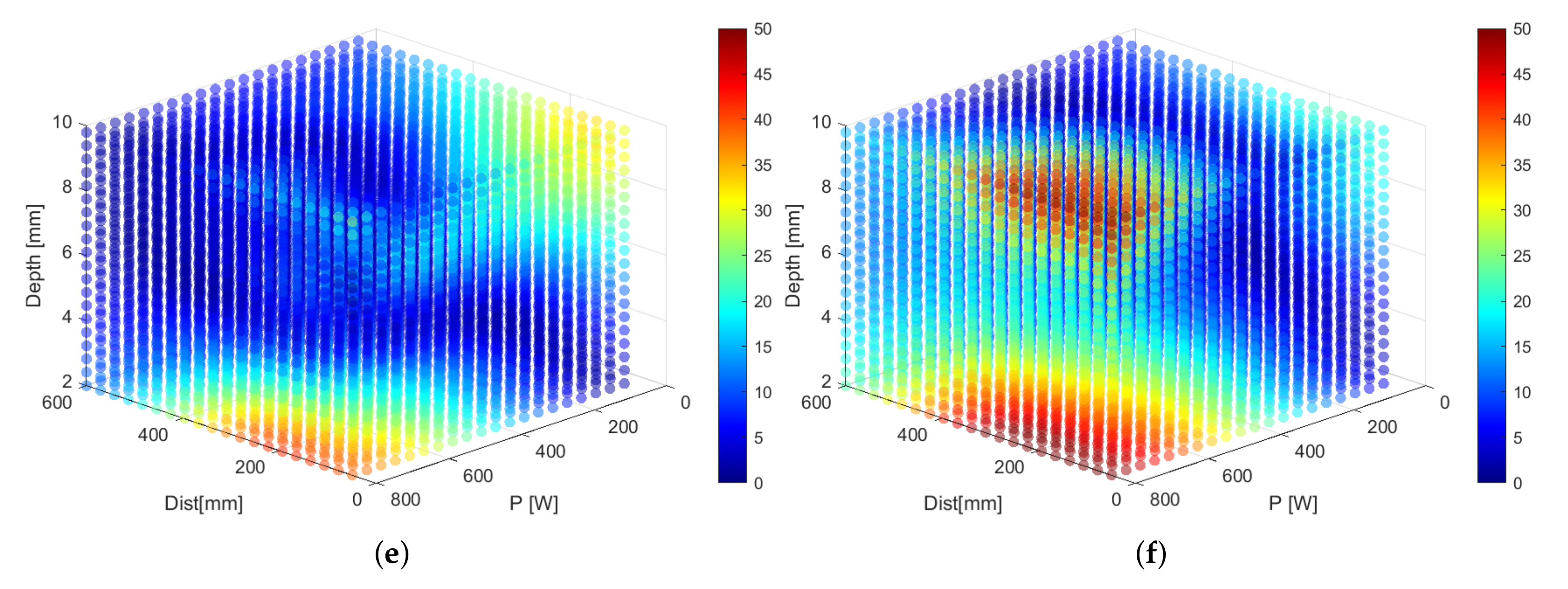
The model can also be used to visualize regions in the input space that result in undesirable temperatures for the sample. For instance, we can highlight regions where the temperature of the sample would become too high. This serves as a warning, as temperatures that are too high might cause damage to the sample under inspection. In Figure 4, we provide an overview of the predicted temperature differences per defect diameter. Regions that are colored are to be avoided when designing the dynamic line scan thermography setup. These plots also reveal that some regions of the input space are workable for some defects, but not for others. The full benefit of these plots comes into its own when using software that allows the end user to rotate the generated cubes, which is trivial to set up in Matlab or any Python environment equipped with a graphing library, such as Matplotlib.
Example 4.
In this last example, we visualize the plots from Example 3 in a different way to highlight regions of the input space that correspond to appropriate temperature differences. In Figure 5, we color regions that result in hard-to-detect (or even undetectable) temperature differences red. For this example, we set the threshold to an arbitrary value of 5 °C. Regions that result in temperature differences above 25 °C are colored yellow. Ideal regions lie in between those values and are given the color green (see Table 2).
Figure 4.
Visualization of the temperature difference for six different defect diameters. (a) 12 mm, (b) 14 mm, (c) 16 mm, (d) 18 mm, (e) 20 mm and (f) 22 mm. Red indicates temperature differences that might result in damaging the sample under inspection. These plots serve as a warning when designing a setup.


Figure 5.
Visualization of the temperature difference for six different defect diameters. (a) 12 mm, (b) 14 mm, (c) 16 mm, (d) 18 mm, (e) 20 mm and (f) 22 mm. Red are temperature differences below 5 °C, yellow above 25 °C and green in between. Only the green regions are of practical value in real-world applications.


Table 2.
Optimal parameter sets found for the examples explained above.
| Parameter | Example 1 | Example 2 | Example 3 | Example 4 |
|---|---|---|---|---|
| Ambient Temperature [°C] | 20 | 20 | 20 | 20 |
| Velocity [mm/s] | 10 | 10 | 10 | 10 |
| Camera Height [mm] | 450 | 450 | 450 | 450 |
| Diameter Hole [mm] | 14 | 12–24 | 22 | 12 |
| Startdepth Hole [mm] | 6 | 2–9.8 | 2–9.8 | 2–9.8 |
| Heating Power [W] | 50 | 500 | 200–400 | 600–800 |
| Distance cam.–heat [mm] | 335–420 | 100 | 500–600 | 50–200 |
Example 1 handles the question ‘What parameter combination should be used to be able to detect a predefined defect with a certain start depth and diameter, with a minimal of amount of heating energy needed?’. Example 2 searches for the best parameter combination to detect as many holes as possible with only adjusting the heating power. Example 3 predicts the regions in the input space that result in undesirable temperatures for the sample. Consequently, the interesting regions can be found as the remaining parameter combinations. Example 4 visualizes the regions of the input space that correspond to appropriate temperature differences. Depending on the colors, one can find a suitable region
4. Discussion
Both the RMSE and the average standard deviation show an initial steep decline that gradually flatlines. All our experiments have shown to converge to the same values after enough iterations. These curves support the decision making process whether or not to continue to add more data points (costly simulations). For our application, one could conclude that after 350 iterations the RMSE and the standard deviation are sufficiently low enough and do not change significantly anymore. The total amount of iterations needed to train the Gaussian process such that it can approximate the simulations up to an adequate level, depends on the application itself. It is a function of the available computational budget and the amount of uncertainty that can be tolerated. Similarly, generating a response surface is also subjective in the sense of deciding when a surrogate has a sufficient resolution and accuracy for the specified application. Therefore this manuscript does not focus on the exact numbers or percentage of data points needed to approximate the response surface.
Simulators and emulators are models of an underlying truth and as such nothing more than an approximation. This means that one has to be prudent about the outcomes of such models. For instance, it is possible for the model to predict values that do not correspond with reality or, even worse, that do not have any physical meaning. For instance, we noticed that for some test points (points were we make predictions) far away from the data, it is possible to obtain negative values for the temperature difference, even though the data only contained positive values. This issue can be dealt with in two ways. First, one could implement constraints on the model. In our case we could alter the covariance function, such that only positive values can be predicted by the model. This is an approach thoroughly explained in [23]. Second, in this research, we chose the Gaussian process for the underlying machine learning model. By following the Bayesian paradigm [9], this stochastic model makes predictions that are not just numerical values (in our case for the temperature difference). They are also accompanied by a variance. As such, each prediction for every test point is in fact a normal distribution. The variance can be interpreted as a measurement of uncertainty about the prediction. This extra information should be taken into account when evaluating the predictions.
As mentioned throughout the text, several optimisations could further improve the performance of the model. They were not investigated in this work, because we wanted to restrict ourselves to a basic implementation of the core idea of approximating dynamic line scan thermography parameter design via emulation. We consider these to be future work. First, the initial sampled points were drawn uniformly from the input space. Several alternatives are described in the literature [12,16,17]. As the total number of sampled points increases, the influence of the initial points becomes less important. Still, on very tight computational budgets, this could become a factor of interest. Second, the Uncertainty Sampling method sometimes favours points on the boundary of the input space. This is due to the fact that the density of data points is lower in those regions and thus the uncertainty is higher (there are no data points beyond the boundary). Integrated Variance Reduction takes this drawback into account and calculates the total amount of uncertainty reduction a new data point yields. It does so for each point in the test set. This reduces the score of points in the vicinity of the boundary. It is to be expected that Integrated Variance Reduction would reduce the number of time consuming sampled input points, but at a higher computational cost. This is also stated in [18]. The effect of this remains an open question. Third, as also stated above, the Gaussian process used in this study can be further developed to incorporate prior knowledge in the form of constraints.
5. Conclusions
We have described a method to emulate the time consuming simulations for a dynamic line scan thermography setup. By means of a Gaussian process, the simulator can be approximated. We have shown that the accuracy increases for every simulation that is added to the training set of the Gaussian process. However, the increase flatlines after a certain application specific number of simulations. At this point, adding more simulations, a time consuming effort, does not add to the overall usefulness of the model. We also posed several parameter design questions relevant in real world engineering design challenges. We demonstrated that a trained emulator can be queried to help find solutions to those questions. This method facilitates the process of finding an economic viable set of design parameters for a dynamic line scan thermography setup in industrial applications.
Author Contributions
Conceptualization, S.V. and I.D.B.; methodology, S.V. and I.D.B.; software, S.V. and I.D.B.; validation, S.V. and I.D.B.; formal analysis, S.V. and I.D.B.; investigation, S.V. and I.D.B.; resources, S.V.; data curation, S.V.; writing—original draft preparation, S.V. and I.D.B.; writing—review and editing, S.V., I.D.B., X.M., R.P., G.S.; visualization, S.V. and I.D.B.; supervision, X.M., R.P., G.S.; project administration, S.V.; funding acquisition, X.M., R.P., G.S. All authors have read and agreed to the published version of the manuscript.
Funding
This research has been funded by Research Foundation-Flanders under grant Doctoral (PhD) grant strategic basic research (SB) 1SC0819N (Simon Verspeek) and the University of Antwerp (BOF FFB200259, Antigoon ID 42339).
Data Availability Statement
The software used for this manuscript as well as the file including the sampled data points can be accessed here: https://github.com/IvanDeBoi/DLST_parameter_design_via_GP_emulation (accessed on 10 February 2022).
Acknowledgments
We thank the anonymous reviewers whose comments helped improve the quality of this paper.
Conflicts of Interest
The authors declare no conflict of interest.
References
- Maldague, X. Nondestructive Evaluation of Materials by Infrared Thermography–Xavier P.V. Maldague; Springer: Berlin/Heidelberg, Germany, 1993. [Google Scholar]
- Verspeek, S.; Gladines, J.; Ribbens, B.; Maldague, X.; Steenackers, G. Dynamic Line Scan Thermography Optimisation Using Response Surfaces Implemented on PVC Flat Bottom Hole Plates. Appl. Sci. 2021, 11, 1538. [Google Scholar] [CrossRef]
- Ibarra-Castanedo, C.; Servais, P.; Ziadi, A.; Klein, M.; Maldague, X. RITA–Robotized Inspection by Thermography and Advanced Processing for the Inspection of Aeronautical Components. In Proceedings of the 2014 Quantitative InfraRed Thermography, Bordeaux, France, 7–11 July 2014. [Google Scholar] [CrossRef]
- Peeters, J.; Verspeek, S.; Sels, S.; Bogaerts, B.; Steenackers, G. Optimised dynamic line scanning thermography for aircraft structures. Quant. InfraRed Thermogr. J. 2019, 16, 260–275. [Google Scholar] [CrossRef]
- Peeters, J.; Ibarra-Castanedo, C.; Khodayar, F.; Mokhtari, Y.; Sfarra, S.; Zhang, H.; Maldague, X.; Dirckx, J.J.; Steenackers, G. Optimised dynamic line scan thermographic detection of CFRP inserts using FE updating and POD analysis. NDT E Int. 2018, 93, 141–149. [Google Scholar] [CrossRef]
- Ringermacher, H.I.; Mayton, D.L.; Howard, D.R. Towards a flat-bottom hole standard for thermal imaging. Rev. Prog. Quant. Nondestruct. Eval. 1998, 17, 425–429. [Google Scholar]
- Frendberg Beemer, M.; Shepard, S. Aspect Ratio Considerations for Flat Bottom Hole Defects in Active Thermography. Quant. InfraRed Thermogr. Conf. 2016, 15, 1–16. [Google Scholar] [CrossRef]
- Paleyes, A.; Pullin, M.; Mahsereci, M.; McCollum, C.; Lawrence, N.D.; Gonzalez, J. Emulation of physical processes with emukit. arXiv 2021, arXiv:2110.13293. [Google Scholar]
- Rasmussen, C.E.; Williams, C.K.I. Gaussian Processes for Machine Learning; The MIT Press: Cambridge, MA, USA, 2006; Volume 38. [Google Scholar]
- Ho, T.K. Random decision forests. In Proceedings of the 3rd International Conference on Document Analysis and Recognition, Montreal, QC, Canada, 14–16 August 1995; Volume 1, pp. 278–282. [Google Scholar] [CrossRef]
- Lim, T.; Wang, K. Comparison of machine learning algorithms for emulation of a gridded hydrological model given spatially explicit inputs. Comput. Geosci. 2022, 159, 105025. [Google Scholar] [CrossRef]
- Noè, U.; Lazarus, A.; Gao, H.; Davies, V.; MacDonald, B.; Mangion, K.; Berry, C.; Luo, X.; Husmeier, D. Gaussian process emulation to accelerate parameter estimation in a mechanical model of the left ventricle: A critical step towards clinical end-user relevance. J. R. Soc. Interface 2019, 16, 20190114. [Google Scholar] [CrossRef] [PubMed]
- Pan, T.; Cai, Y.; Chen, S. Development of an Engine Calibration Model Using Gaussian Process Regression. Int. J. Automot. Technol. 2021, 22, 327–334. [Google Scholar] [CrossRef]
- Liu, D.C.; Nocedal, J. On the limited memory BFGS method for large scale optimization. Math. Program. 1989, 45, 503–528. [Google Scholar] [CrossRef] [Green Version]
- Kristjanson Duvenaud, D.; College, P. Automatic Model Construction with Gaussian Processes Declaration. Available online: https://www.cs.toronto.edu/~duvenaud/thesis.pdf (accessed on 10 February 2022).
- Fang, K.T.; Li, R.; Sudjianto, A. Design and Modeling for Computer Experiments; Chapman and Hall/CRC: Boca Raton, FL, USA, 2005. [Google Scholar]
- Jones, D.R.; Schonlau, M.; Welch, W.J. Efficient Global Optimization of Expensive Black-Box Functions. J. Glob. Optim. 1998, 13, 455–492. [Google Scholar] [CrossRef]
- Sacks, J.; Welch, W.J.; Mitchell, T.J.; Wynn, H.P. Design and Analysis of Computer Experiments. Stat. Sci. 1989, 4, 409–423. [Google Scholar] [CrossRef]
- Buisson-Fenet, M.; Solowjow, F.; Trimpe, S. Actively learning gaussian process dynamics. In Proceedings of the 2nd Conference on Learning for Dynamics and Control, Online, 11–12 June 2020; pp. 5–15. [Google Scholar]
- Pasolli, E.; Melgani, F. Gaussian process regression within an active learning scheme. In Proceedings of the 2011 IEEE International Geoscience and Remote Sensing Symposium, Vancouver, BC, Canada, 24–29 July 2011; pp. 3574–3577. [Google Scholar] [CrossRef]
- Gessner, A.; Gonzalez, J.; Mahsereci, M. Active multi-information source Bayesian quadrature. In Proceedings of the 35th Uncertainty in Artificial Intelligence Conference, Tel Aviv, Israel, 22–25 July 2019; pp. 712–721. [Google Scholar]
- Oladyshkin, S.; Mohammadi, F.; Kroeker, I.; Nowak, W. Bayesian3 Active Learning for the Gaussian Process Emulator Using Information Theory. Entropy 2020, 22, 890. [Google Scholar] [CrossRef] [PubMed]
- Swiler, L.P.; Gulian, M.; Frankel, A.L.; Safta, C.; Jakeman, J.D. A survey of constrained Gaussian process regression: Approaches and implementation challenges. J. Mach. Learn. Model. Comput. 2020, 1, 119–156. [Google Scholar] [CrossRef]
Figure 1.
Visualization of the finite element simulation consisting of a flat bottom hole plate (blue) and a line heater (yellow). The line heater moves above the sample in a linear motion. For a more detailed figure and explanation, we refer the reader to [2].
Figure 1.
Visualization of the finite element simulation consisting of a flat bottom hole plate (blue) and a line heater (yellow). The line heater moves above the sample in a linear motion. For a more detailed figure and explanation, we refer the reader to [2].

Figure 2.
Response surface as generated in [2]. The surface is generated from 1000 finite element simulations, using eight input parameters. The simplified response surface has all input parameters fixed, except for the heat load and the source velocity. The fixed parameters are: = 425 mm, = 5.8 mm, = 9 mm, = 430 mm, = 48 C. Using this response surface, one can find the best temperature difference as a valley or top.

Figure 3.
Graphical visualization of the learning process of the Gaussian process for 5 runs of 500 iterations. (a) represents the root mean square error (RMSE) of the learned surrogate compared to the response surface created in [2]. (b) shows the average standard deviation of the Gaussian process posterior prediction.

Table 1.
Hyperparameters of the trained Gaussian processes.
| Run | [mm] | [W] | [mm] | [mm] | |
|---|---|---|---|---|---|
| 1 | 142.81 | 246.17 | 2.28 | 2.35 | 11.97 |
| 2 | 150.00 | 255.99 | 2.30 | 2.41 | 11.75 |
| 3 | 182.72 | 216.52 | 2.23 | 1.98 | 10.87 |
| 4 | 177.48 | 223.02 | 2.26 | 1.96 | 10.97 |
| 5 | 153.98 | 238.46 | 2.60 | 2.37 | 12.84 |
The values for the hyperparameters of the covariance function of the trained Gaussian processes for each of the five runs
Publisher’s Note: MDPI stays neutral with regard to jurisdictional claims in published maps and institutional affiliations. |
© 2022 by the authors. Licensee MDPI, Basel, Switzerland. This article is an open access article distributed under the terms and conditions of the Creative Commons Attribution (CC BY) license (https://creativecommons.org/licenses/by/4.0/).
Share and Cite
MDPI and ACS Style
Verspeek, S.; De Boi, I.; Maldague, X.; Penne, R.; Steenackers, G. Dynamic Line Scan Thermography Parameter Design via Gaussian Process Emulation. Algorithms 2022, 15, 102. https://0-doi-org.brum.beds.ac.uk/10.3390/a15040102
AMA Style
Verspeek S, De Boi I, Maldague X, Penne R, Steenackers G. Dynamic Line Scan Thermography Parameter Design via Gaussian Process Emulation. Algorithms. 2022; 15(4):102. https://0-doi-org.brum.beds.ac.uk/10.3390/a15040102
Chicago/Turabian StyleVerspeek, Simon, Ivan De Boi, Xavier Maldague, Rudi Penne, and Gunther Steenackers. 2022. "Dynamic Line Scan Thermography Parameter Design via Gaussian Process Emulation" Algorithms 15, no. 4: 102. https://0-doi-org.brum.beds.ac.uk/10.3390/a15040102
Note that from the first issue of 2016, this journal uses article numbers instead of page numbers. See further details here.