
An LSM-Tree Index for Spatial Data

Faculty of Electrical Engineering and Computer Science, Ningbo University, Ningbo 315211, China
*
Author to whom correspondence should be addressed.
Algorithms 2022, 15(4), 113; https://0-doi-org.brum.beds.ac.uk/10.3390/a15040113
Submission received: 22 February 2022
/
Revised: 19 March 2022
/
Accepted: 24 March 2022
/
Published: 25 March 2022
(This article belongs to the Section Databases and Data Structures)
Abstract
:An LSM-tree (log-structured merge-tree) is a hierarchical, orderly and disk-oriented data storage structure which makes full use of the characteristics of disk sequential writing, which are much better than those of random writing. However, an LSM-tree can only be queried by a key and cannot meet the needs of a spatial query. To improve the query efficiency of spatial data stored in LSM-trees, the traditional method is to introduce stand-alone tree-like secondary indexes, the problem with which is the read amplification brought about by dual index queries. Moreover, when more spatial data are stored, the index tree becomes increasingly large, bringing the problems of a lower query efficiency and a higher index update cost. To address the above problems, this paper proposes an ER-tree(embedded R-tree) index structure based on the orderliness of LSM-tree data. By building an SER-tree(embedded R-tree on an SSTable) index structure for each storage component, we optimised dual index queries into single and organised SER-tree indexes into an ER-tree index with a binary linked list. The experiments showed that the query performance of the ER-tree index was effectively improved compared to that of stand-alone R-tree indexes.
1. Introduction
In modern LSM-tree-based storage architecture [1], the SSTable structure is mainly used as the storage component on disk, initially proposed in BigTable [2]. This paper takes RocksDB as an example to show the design pattern of the modern LSM tree. The components in memory include MemTable, Immutable Memtable; the components in the disk include the SSTable file, log file, current file and manifest file. When a user writes a KV record, RocksDB will save the record in the log file first and then insert the record into MemTable in memory. RocksDB does not directly reside the latest data in the disk for each writing operation but splits it into a sequential write to the log file and in-memory-based data insertion. When the memory’s MemTable is oversized, RocksDB generates a static snapshot of Immutable MemTable and generates a new MemTable to receive the latest update. The backend scheduling thread is responsible for flushing this snapshot to Level 0 on disk for persistent storage as an SSTable. This process is called minor compaction. When the file size of a layer on the disk reaches a specific size, the system compresses and merges it with several SSTables in the next layer and the newly generated SSTable resides in the next layer. This process is called major compaction. LSM-trees are a widely used storage structure for NoSQL (Not Only SQL) databases, including Google’s BigTable [2], LevelDB [3], Apache’s HBase [4] and AsterixDB [5], Facebook’s RocksDB [6] and Cassandra [7] and are widely used in writing-intensive scenarios.
However, a traditional LSM-tree index can only query data by key, not directly by value and thus cannot be used for spatial data to perform effective location-based range queries and other operations by spatial coordinates in the value. To address the above problem, spatial data query operations on LSM-trees can be accomplished by mapping the two-dimensional spatial location in the value into one dimension as the key through the space-filling curve method [8]. However, this method may place pressure on the system’s computational resources in data mapping [9]. Some approaches involve introducing a tree-like auxiliary index [10,11,12,13], storing the two-dimensional data location information on the tree-like auxiliary index and when querying, after using the location information to query the auxiliary index to obtain the key of the data, then going to the LSM-tree to query the complete data <key, value> using the key. However, the disadvantage is that when the LSM-tree is merged, the entire auxiliary index tree needs to be updated and the update cost is considerable. Moreover, during the query, the key should be obtained from the secondary index first and then the complete data should be obtained by applying the key to the LSM-tree. Such dual index querying leads to significant reading amplification. Although the read amplification problem can be alleviated by improving the LSM read performance, such as the LSM-tree tidal structure [14] and multi-threaded parallel querying [15], it still does not fundamentally solve the mechanical problem of a secondary index query [16]. An R-tree index is the most widely used spatial index among tree-like auxiliary indexes and its query performance is stable and applicable to a wide range of data types. Suppose we can solve the dual index query, index update and multiplex query problems arising from its application to LSM-trees. In this case, we can significantly improve the query performance of spatial data on LSM-trees.
- We propose a new spatial data index SER-tree (embedded R-tree on an SSTable), introduce Hilbert spatial data sorting, and combine an R-tree index with an SSTable to reduce the read amplification caused by R-tree multiplex queries and dual index queries.
- Based on an SER-tree, we present an ER-tree (embedded R-tree) on LSM to further improve the index query and the update efficiency by organising the SER-tree hierarchically through a binary linked list.
- We implemented the ER-tree index structure for spatial data on the open-source NoSQL database RocksDB. By experimenting with a stand-alone LSM R-tree index, we conclude that there is a better improvement in query performance.
The remainder of this paper is organised as follows: Section 2 briefly introduces the current work related to spatial data indexing on LSM-trees and our motivation for improvement; Section 3 presents the implemental details of the ER-tree index; Section 4 introduces query algorithms on ER-tree indexes; Section 5 tests the build and query performance of the ER-tree indexes through experiments; Section 6 concludes the work of this paper.
2. Related Works
An LSM-tree is a storage structure commonly used in NoSQL databases to improve data writing performance. However, finding data in an LSM-tree is realised by the key, which cannot directly provide spatial range query operations. Therefore, suitable spatial data indexes must be designed for an LSM-tree structure. This section briefly introduces the basic structure of LSM-trees. It analyses the current work related to spatial data indexing on LSM-trees, which leads to the necessity of the work in this paper.
2.1. LSM-Tree Structure
The basic structure of an LSM-tree [17] is shown in Figure 1. When a writing operation arrives, it first caches data in the memory MemTable. When the memory is complete, it turns the MemTable into an immutable MemTable and then immediately flushes the immutable MemTable to the disk through a minor compaction operation to achieve sequential I/O processes and avoids the significant system overhead caused by random I/O. Moreover, to improve the read performance, the LSM-tree performs a major compaction operation according to the storage situation of SSTable in the disk to reduce the redundancy of the data stored there and to retain the data of an SSTable in the same layer in order by the key. The key range does not overlap (except the level 0 layer).
2.2. Related Work
In terms of the single-dimensional indexing of LSM-trees, HBase database [4] uses skip-list for memory and B+ tree for external storage to implement a B+ tree index based on LSM-trees (LSM B-tree) based on the original LSM-trees to achieve efficient read and writing performance. Sears [18] improved the original LSM-trees to build a fusion tree of LSM-trees and B+ trees (bLSM-tree), which solves the read amplification and writing blocking problems of the original LSM-trees. However, these two methods are only suitable for processing one-dimensional data and some special processing is required for multi-dimensional data.
In terms of multi-dimensional indexing of LSM-trees, Lawder et al. [8] proposed two spatial indexes, namely, dynamic Hilbert B+ tree (DBH-tree) and dynamic Hilbert-valued B+ tree (DBVH-tree), using B+ trees and Hilbert curves to store spatial data. Both spatial indexes can be applied well to LSM-trees to solve the problem of LSM-trees only being able to index single-dimensional data. However, the shortcoming is that LSM B-trees based on the Hilbert curve can only index points, so these approaches are only applicable to point data, not line or surface data.
AsterixDB [5] is an open-source database based on LSM-trees with a native secondary index for spatial data. An R-tree index [19] is a widely used spatial data index. The database uses an LSM R-tree [12] for spatial range queries. In Kim’s [20] experiments comparing several LSM-tree spatial indexes based on the AsterixDB database, an LSM R-tree has better stability in data query performance and update efficiency compared to a DBH-tree, DHVB-tree, or SHB-tree and is suitable for various types of spatial data. However, the overall design maintains a stand-alone R-tree index on the disk. The index update needs to find the changed key-value pairs and update them to the R-tree index in turn, which has the problem of slow index updates. A compaction operation of SSTables on an LSM-tree causes many index update operations on an R-tree, which increases the disk I/O overhead. Moreover, its index storage is independent of each SSTable. When the data key is queried on the secondary index, it still needs to query the LSM-tree primary index to obtain the complete data <key, value> by the key. This dual index query increases the read amplification and reduces the efficiency of spatial data queries. There is also a problem with the R-tree itself, because the MBR (minimal bounding rectangle) on the leaf nodes overlap, resulting in the R-tree making multiway queries when querying, further reducing the query efficiency. Figure 2 is a typical implementation of an R-tree index on an LSM-tree. Such an index design scheme with stand-alone storage of the index and data suffers from the problems of a low query efficiency and a costly index update and this paper calls this structure a stand-alone R-tree index.
Liu [10] and Rui [11] improved the LSM R-tree using a hierarchical index. They designed a corresponding secondary index for the MemTable and L0 (Level 0) individually, used a large R-tree to store the index of the SSTable of L1 and above and finally formed a three-layer structure of the index. This improves the query performance of an LSM R-tree to a certain extent but suffers from the same problem as stand-alone R-tree indexes, having a dual index query problem.
A reduction in the index update cost and the system read amplification in the combination of LSM R-trees is the direction many researchers focus on. A RUM-tree [21] is a structure that handles frequently updated spatial data using an update memo structure. An LSM RUM-tree [22] uses a RUM-tree to store and process update-intensive spatial data. It introduces the update memo into the LSM R-tree index, reduces the complexity of index deletion and update and improves the performance of data queries. The problem of reading amplification can be partially solved in traditional ways to improve the performance of LSM-tree reading, such as an LSM-tree tidal structure [14] and a multi-threaded parallel query [15]. In the tidal structure, Wang et al. moved the files frequently visited in the bottom to a higher position, reducing the data reading delay and thus reducing the system read amplification. In the multi-threaded parallel query method, Cheng et al. used multithreading to read the last layer and other layers of LSM to improve the efficiency of the data query. Although both ways can enhance the data query efficiency and reduce the system read amplification, they do not fundamentally solve the dual index query mechanism. In this regard, Li et al. proposed a decoupled secondary index [23], whose query process avoids obtaining records from the primary index, thus effectively reducing the system read amplification and improving the data query performance.
Through the above elaboration, it can be concluded that the advantages of the LSM R-tree index are high computational efficiency, stable data query performance and wide suitable data types. However, due to the maintenance of a stand-alone R-tree index, there is still much room for optimisation in reducing the cost of reading amplification and update. Further improvements include: (1) reducing the read amplification caused by the dual index query mechanism; (2) reducing the update cost on many R-tree indexes caused by compaction operations; (3) for R-tree itself, reducing the query overhead caused by multiway queries.
Therefore, this paper proposes an ER-tree index to construct an embedded R-tree index of an LSM-tree based on the SER-Tree index. Each SSTable maintains an SER-tree index and the SER-tree index directly points to the corresponding record on the SSTable, avoiding dual index queries and reducing the read amplification. Furthermore, only the SER-tree indexes involved in the compaction operation are updated, reducing the update overhead. In the organisation of an SER-tree, the spatial data are sorted and the SER-tree is constructed from the bottom up to minimise the MBR overlap and the redundant query overhead caused by multiway queries.
3. SER-Tree Index
As analysed in Section 2, the LSM R-tree index has three improvements: Reducing the multiway queries of R-tree, improving the dual index query mechanism and reducing the update overhead of the R-tree index caused by the compaction operation of an LSM-tree. This section presents the details of the ER-tree index implementation for improvements. In Section 3.1, this paper proposes the design idea of an SER-tree to reduce the multiway query of an R-tree; in Section 3.2, this paper offers to build an ER-tree index on an LSM-tree based on an SER-tree, to improve the dual index query mechanism of the LSM R-tree index and to reduce the update overhead of the R-tree index on an LSM-tree.
3.1. SER-Tree Index Design
The KV database based on an LSM-tree is usually composed of the MemTable and immutable MemTable resident in memory. The other is the disk divided into multiple layers in storage logic. Each disk layer contains multiple SSTable files and the key-value data are encapsulated in these SSTable files. Except for the disk level 0 layer, the data stored in each layer are arranged in the key order and the range of keys between each SSTable is not overlapped.
In the SSTable file, the data are divided into several data blocks, as shown in Figure 3. The data in the data blocks are arranged in dictionary order by the key acquiescently, but users can also define their ordering of keys. Because each SSTable in each layer of the LSM-tree is divided according to the range of the key and the data in an SSTable are stored in the order of the key, if the key can be designed reasonably, the data adjacent to the geographical location may be stored together, which is convenient for building indexes for efficient spatial range queries and other operations.
Suppose we follow the traditional LSM R-tree indexing idea and build the R-tree index directly on the value, the read performance will be degraded due to the unclear relationship between the location of the value and the R-tree index that cannot reflect the orderliness of the data in the LSM-tree itself. Precisely, assuming a range query obtains the key from the R-tree index first and then the complete data from the LSM-tree by finding the key, it scans the SSTable in the disk file one by one, because it does not know which SSTable the data corresponding to the key is stored in. Although the LSM-tree itself has a Bloom filter, a key binary query and other ways to accelerate the query, these query overheads cannot be ignored once the amount of data increases. If there is an effective way to organise spatial data so that each query does not need to scan disk files sequentially, the query performance will be further improved.
In this paper, the Hilbert values of the spatial location in the data are encoded as the key and the spatial data can be stored in the SSTable in Hilbert order. When a range query is performed, the data can be directly retrieved through the data storage location mapped by the SER-tree index to avoid dual index queries.
The SER-tree learns from the idea of a Hilbert R-tree. The traditional R-tree is built by the top-down dynamic interpolation method. Because the node splitting process is locally optimised, it inevitably increases the MBR overlapping area of spatial objects. For the SSTable structure in the LSM-tree, the data in it do not change once generated. When selected for compaction, several SSTables are merged into a new SSTable. Therefore, for the SSTable index, the bottom-up batch loading method is more suitable. In the process of generating leaf nodes, the spatial objects can be arranged in Hilbert’s order first. Then, a series of consecutive spatial objects can first be pressed into the tree’s leaf nodes by scanning the sorted list and then pressed into the next leaf node until all spatial objects are processed. Finally, a complete Hilbert R-tree is generated from the bottom up. The bottom-up Hilbert R-tree can be close to 100% in spatial storage efficiency and can reduce the redundant queries caused by multiway queries to a certain extent, which is suitable for indexing applications that do not need to insert and delete data frequently, such as an SSTable. Figure 4 shows an MBR comparison between the Hilbert R-tree and the R-tree. It shows that the Hilbert R-tree has a lower MBR overlapping area than the traditional R-tree.
3.2. SER-Tree Index Build
The following describes how to build an SER-tree index on an SSTable. First, we assume that the key and value are of a fixed size, the key is the Hilbert value of the coordinates in the spatial data and the value is the spatial data information. If the size is not specified, one can refer to the method of WiscKey [24] and can use the technique of value log to store the key and value separately, while the key is the Hilbert value and the value is the pointer to the location of that data in the value log.
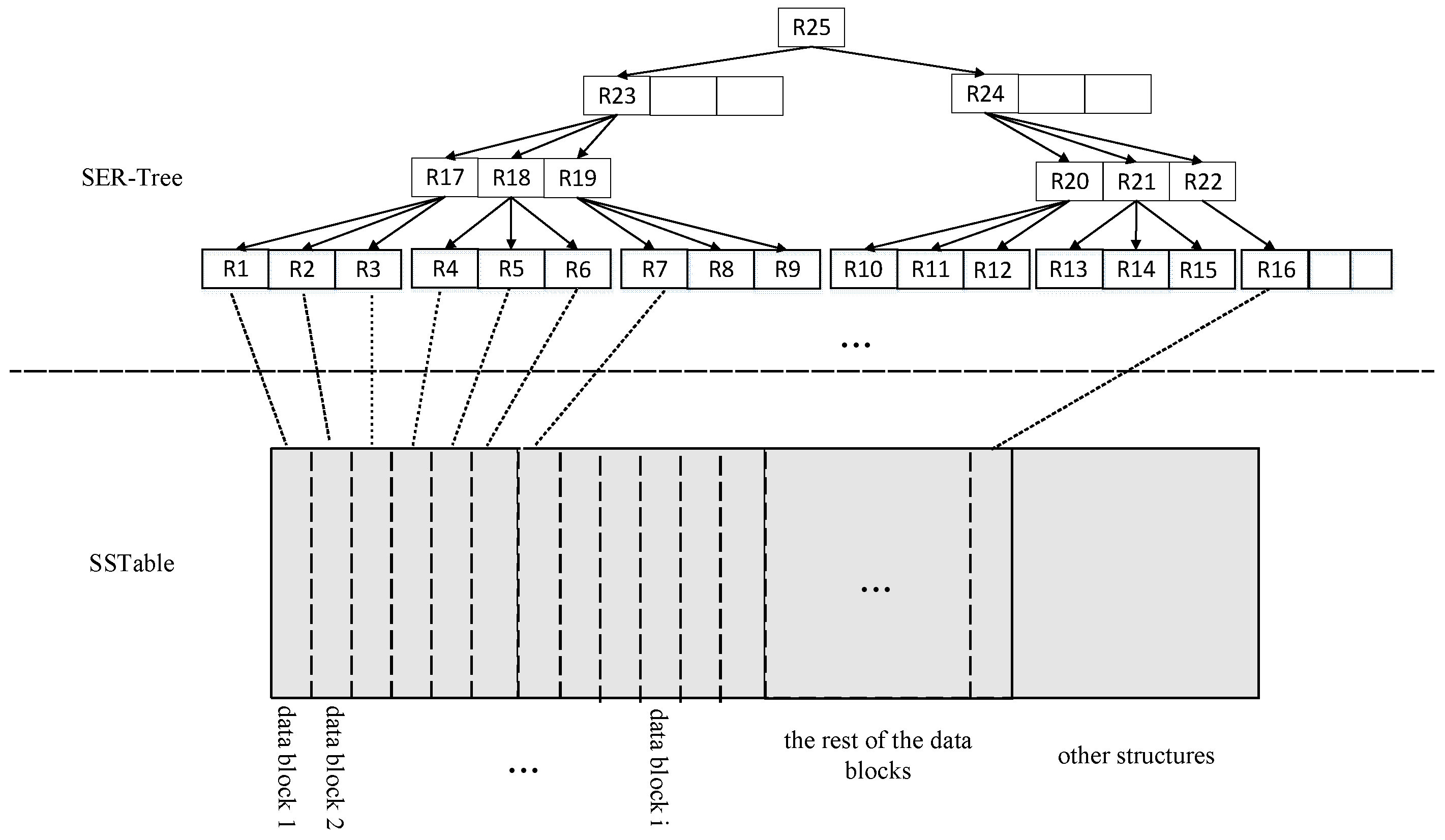
The corresponding SER-tree index for each SSTable is then built and each data block in that SSTable, corresponding to a leaf node in the SER-tree index, is defined as follows:
where is the minimum bounding rectangle of the spatial data in the data block and db_ptr is a pointer to the corresponding data block, as shown in Figure 5 (R1–R16).
After building the leaf nodes, the middle nodes of the SER-tree are built from the bottom up, as shown in Figure 5 (R17–R22). The middle nodes of the SER-tree are defined as:
where cMBR is the minimum bounding rectangle covering all child nodes in the middle node and child_ptr is the set of pointers to the next level of child nodes.
The SER-tree is built from the bottom up according to the pre-set node size of the SER-tree, up to the root node of the SER-tree. The root node is defined as:
where tMBR is the minimum bounding rectangle covering all child nodes in the root node T, child_ptr is the set of pointers of the node to the next level of child nodes and the next pointer is the SER-tree index pointing to the adjacent SSTable. At this point, the SER-tree index on the SSTable is built, as shown in Figure 5.
The SER-tree index construction algorithm is proposed based on the above structure, as shown in Algorithm 1.
| Algorithm 1 SER-tree build algorithm |
| Input: S: SSTable; k: the capacity of SER-Tree node. Output: T: an SER-Tree on SSTable. 1: Q ← ∅; // Q: auxiliary queue 2: for each data block in S, do 3: Build a leaf node N to store the data points in a data block; 4: Q.enqueue (<N,1>); 5: end for 6: while Q.size ()>1 do 7: Dequeue the first k nodes of the same level t from Q; //t: the level of SER-Tree 8: Build a node N to store MBRs of the nodes and pointers of the nodes; 9: Q.enqueue (<N,t+1>); 10: end while 11: T ← Q.LastNode; 12: return T; |
Algorithm 1 describes the process of building an SER-tree index. The auxiliary queue Q is represented as a <N,t> binary, where N represents the leaf nodes and t represents the level of the node in the SER-tree. In the first step, Algorithm 1 builds leaf nodes N for each data block in turn and then pushes them into the queue Q (lines 2–5). In the second step, for the nodes on the same level t in the queue Q, a middle node is built for every k node and the middle node stores the MBRs and pointers of the child nodes; the above operation is repeated until the size of the queue becomes one (lines 6–10). Finally, the last node of the queue Q is deposited into and stored in T, completing the algorithm (lines 11–12).
4. ER-Tree Index
We first built the SER-tree index on each SSTable and then linked the SER-tree indexes on each layer of the LSM-tree to build the ER-Tree index on LSM. The following described the ER-tree index building method on the LSM-tree. In Section 4.1, this paper presents the design idea of the ER-tree; in Section 4.2, this paper explains the building method of the ER-tree; in Section 4.3, this paper proposes further improvements for the ER-tree; in Section 4.4, this paper presents query algorithms based on the ER-tree index, including point query, rectangular range query and prototype range query.
4.1. ER-Tree Index Design
The traditional R-tree index of spatial data on an LSM-tree uses the method of indexing multiple SSTables by a single file to reduce the number of index files, which simplifies the design, but reduces the data query efficiency and increases the index update overhead. In this paper, a single index file is used to maintain a single SSTable. Although many index files are added, the cost of index update can be reduced when the compaction operation occurs because only a few indexes on SSTable are updated. In terms of data querying, since the related records are available on the SSTable corresponding to the index, there is no need to perform dual index queries, which reduces the read amplification and improves the spatial data query performance.
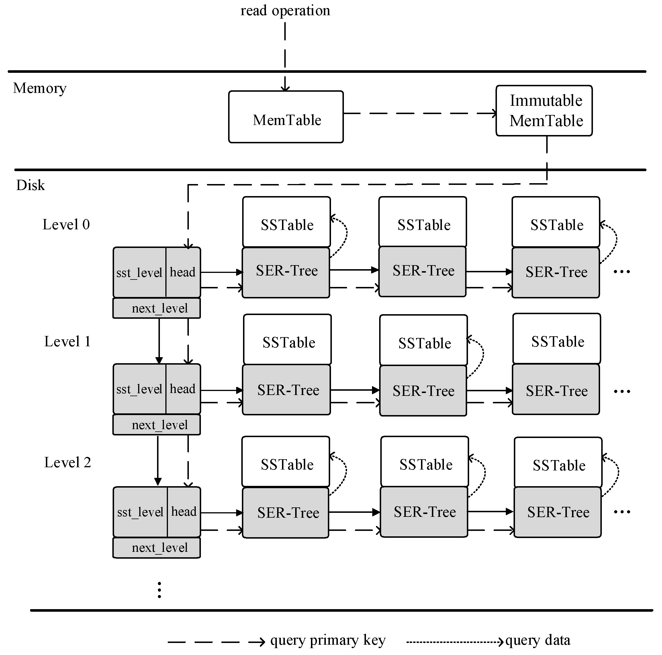
In the external storage of an LSM-tree, the storage structure is logically divided into several layers and each layer contains multiple SSTable files. To avoid scanning the SER-tree indexes on each SSTable, the indexes need to be organised according to the hierarchical idea of LSM-trees to improve the efficiency of the data query. Figure 6 shows the ER-tree index structure of the spatial data on the LSM-tree designed in this paper and the details of the build method are presented in Section 4.2. The SER-tree on the SSTable in each level of the external storage LSM-tree is organised into a linked list by connecting all the root nodes of the SER-tree at the level and then the headers of all the level lists are organised into a linked list. The formed double linked list organises all the SER-tree indexes on the SSTable together. The query can be filtered by the tMBR range of each node on the double linked list level by level and can filter some SER-tree indexes unrelated to the query scope to avoid scanning all indexes.
4.2. ER-Tree Index Build
Figure 6 shows the ER-tree index structure of the spatial data on the LSM-tree, where the head node of the double linked list is defined as follows:
where sst_level indicates the level where the linked list is located, the head pointer points to the SER-tree index of the first SSTable at that level and the next_level pointer points to the next level of the linked list.
When the LSM-tree is in major compaction operation, the database selects several SSTable files with overlapping keys in levels i and i + 1 for compaction and then outputs the new SSTable files to level i + 1. Accordingly, indexes also need similar compaction operations. When the compaction operation of the LSM-tree is completed, the SER-tree index on the new SSTable is built and the SER-tree index on the compacted SSTable is deleted. After the above steps are finished, the linked list nodes on the ER-tree structure are updated, the old nodes are deleted and the nodes are inserted.
4.3. ER-Tree Index Improve
The above describes the general structure of an ER-tree index, but it is not suitable for practical applications for the following reasons:
- For read-only workloads, ER-tree indexes can provide higher query performance. However, for mixed read-write workloads, the indexes are constantly updated with frequent data writing, resulting in increased overheads, which does not seem to work well with the high writing performance of the LSM-tree structure. However, although writing changes the structure of the LSM-tree, most of its structure remains unchanged, especially for the SSTable in the high levels and a large amount of writing does not cause compaction operations to occur in the high-level SSTable. Therefore, indexes built on these high-level SSTables are effective and improve the data query performance. However, for a low-level SSTable, the data change process is faster and whether to build SER-tree indexes on them needs further analysis.
- In the LSM-tree, many SSTable files have a short lifetime, especially for a low-level SSTable and when a large amount of writing occurs, they are quickly compacted to the next-level SSTable and their lifetime is less than the index build time. Therefore, it is necessary to set a threshold value. If the lifetime of an SSTable file is less than this threshold, there is no need to build an SER-tree index. In this paper, we experimentally measured that for a 4MB SSTable file and the time to build its index was approximately 45 ms. Therefore, we set a time threshold of Tw = 50 ms. If the lifetime of the SSTable is greater than Tw, then the index is built for the SSTable; otherwise, it is not built.
- In addition to the above issues, it is also necessary to consider that even if an SSTable file has a long lifetime, it is not urgent to build indexes on it if there are almost no query tasks. To build an SER-tree index for an SSTable, we need to consider the query gain and the building loss from the index, which are denoted by Gindex and Lindex, respectively, in this paper. If Gindex is larger than Lindex, it means that it is appropriate to build an SER-tree index on this SSTable and if Gindex is smaller than Lindex, it is not applicable to build an index on this SSTable.
If we do not consider the impact of the index building process on other operations of the LSM-tree, the value of Lindex is approximately equal to the index building time, which is denoted by Tbuild in this paper. In this paper, Tbuild is the time to build a Hilbert R-tree index on an SSTable and its size is proportional to the amount of data in the SSTable file. It is calculated by multiplying the average time to build a Hilbert R-tree index for one data point in the offline case by the number of data points in the SSTable file. Gindex is calculated by the time difference between the SER-tree index query time and the baseline method query time. The baseline method is a key binary query of an SSTable without indexing. In this paper, the SER-tree index query time is defined as Tmodel and the baseline method query time is defined as Tbaseline. Assuming that an SSTable has Q queries in its life cycle, the formula for calculating Gindex is shown below:
The data in the above equation cannot be obtained directly from the SSTable file, but rather need to be obtained from the rest of the SSTable files in the same layer that have undergone the entire lifetime, which is defined as SSTel in this paper. Tbaseline is approximately equal to the average baseline method query time on the SSTel file before indexing. Tindex is roughly equivalent to the average index query time on the SSTel file, while Q is the number of queries on the SSTel file.
To sum up, an index build decider (IBD) is needed to judge the timing of the index building. The IBD first selects the SSTable whose lifetime is greater than Tw, then calculates its Gindex and Lindex. If Gindex > Lindex, an SER-tree index is established for the SSTable; otherwise. the index waits to be built. Suppose many SSTables meet the index build conditions simultaneously; in this case, the IBD builds the index according to the value of Gindex − Lindex and the larger the value is, the quicker it will be built to ensure the index achieves the maximum gain.
4.4. ER-Tree Index Query
In this paper, the most significant difference between the query process of the ER-tree index and the stand-alone R-tree index is that the index is built directly on the SSTable, so that when querying, you can go to its corresponding SSTable to obtain the data<key, value>, without the need for a dual query in the way of the stand-alone R-tree index, which reduces the query number and improves the query performance. Figure 7 shows the flow of querying data from the stand-alone R-tree index. First, according to the sparse dashed arrow in the figure, the key is queried on the R-tree using spatial location. After obtaining the key, the data are queried from the LSM-tree again according to the dense dashed arrow, which is a more tedious and time-consuming dual query process. Figure 8 shows the flow of querying data from the ER-tree index; first, according to the sparse dashed arrows in the figure, querying on the ER-tree using spatial location and then directly querying data on the corresponding SSTable according to the dense dashed arrows after querying, which avoids the dual index query compared with the stand-alone R-tree index.
Based on the above ER-tree index, this paper proposes point query, rectangular range query and circle range query algorithms for spatial data on the ER-tree index.
4.4.1. Point Query
The point query of spatial data is based on one or several query coordinate points to query the data in the database with the exact data coordinates as the query coordinate points. The key-value entry is first obtained by a spatial location query on the ER-tree index and then directly through the SSTable corresponding to the index. The point query algorithm on the ER-tree index is shown in Algorithm 2.
| Algorithm 2 Point query algorithm |
| Input: QP: query point, ERT: LSM ER-Tree index Output: result: <key, value>, whose value= QP 1: level_ptr ← ERT. head; 2: while(level_ptr! = null) do 3: ptr ← level_ptr. head; 4: while(ptr! = null) do 5: if include(ptr.tMBR, QP) then //include: judge whether the point QP is within the MBR range 6: LeafNode ← QPFindLeaf (ptr.SERT, QP); //SERT: SER-Tree index on SSTable 7: temp_result. append (LeafNode.db_ptr); 8: end if 9: ptr ← ptr.next; 10: end while 11: level_ptr ← level_ptr.next_level; 12: end while 13: foreach(<key, value>in temp_result) 14: if equals(value, QP) then 15: result. append(<key, value>); end if 16: end for 17: return result; 18: function QPFindLeaf (T, QP) 19: begin 20: if T is a LeafNode, then 21: if include(T.mbr, QP), then 22: return T; else return ∅; 23: else 24: for each child u of T, do 25: if(include (u.mbr, QP)) then 26: QPFindLeaf (u, QP); end if 27: end for 28: end function |
Algorithm 2 describes the process of the ER-tree index point query. In the first step, the ER-tree is used to judge, layer by layer, whether the QP is located in the tMBR of each SER-tree root node in the ER-tree. If it exists, the QPFindLeaf function is executed to obtain the data <key, value> from the data block on the corresponding SSTable and to store it in the temp_result collection (lines 1–12). The second step is to iterate, through the temp_result collection, to judge whether <key, value> in the temp_result collection equals the QP. If it is equal, it is stored in the result collection (lines 13–17); lines 18–28 refer to the QPFindLeaf function, which uses a recursive way to query the leaf node of the MBR containing the query point QP.
4.4.2. Rectangular Range Query
The rectangular range query of spatial data is used to query the data within the rectangular range of coordinate points based on a pair of coordinate points (x1, y1) (x2, y2), where (x1, y1) are the coordinates of the lower-left corner of the rectangle and (x2, y2) are the coordinates of the lower right corner of the rectangle. First, we need to query the data by the coordinate points on the index and then obtain the <key, value> on the corresponding SSTable. The ER-tree index rectangular range query algorithm is shown in Algorithm 3.
| Algorithm 3 Rectangular range query algorithm |
| Input: QR: query spatial range, ERT: LSM ER-Tree index. Output: result_c: <key, value>collection, whose value in QR1. Level_ptr ← ERT. head; 1: level_ptr ← ERT. head; 2: while(level_ptr! = null) do 3: ptr ← level_ptr. head; 4: while(ptr! = null) do 5: if intersect (ptr. tMBR, QR) then // intersect: judge whether the range QR is within or intersects the MBR 6: LeafNode ← QRFindLeaf (ptr.SERT,QR); //SERT: SER-Tree index on SSTable 7: temp. append(LeafNode.db_ptr); end if 8: ptr ← ptr. next; 9: end while 10: end while 11: foreach(<key, value>in temp) 12: if(include(QR, value)) then //include:judge whether the point value is within the QR range 13: result_c. append(<key, value>); end if; 14: end for 15: return result_c; 16: function QRFindLeaf (T, QR) 17: begin 18: if T is a LeafNode, then 19: if (intersect(T.mbr, QR)) then 20: return T; else return ∅; 21: else 22: for each child u of T, do 23: if(intersect(u.mbr, QR)) then 24: QRFindLeaf (u, QR); end if; 25: end for 26: end function |
Algorithm 3 describes the process of the ER-tree index rectangular range query. In the first step, the ER-tree is used to judge, layer by layer, whether the QR intersects (or contains) the tMBR of each SER-tree root node of the ER-tree; if it satisfies this, the QRFindLeaf function is executed to obtain the data <key, value> from the data block on the corresponding SSTable and deposits it into the temp collection (lines 1–10). In the second step, iteration through the temp collection is used to determine whether the value of <key, value> is located in the QR. If it is, it is stored in the result_c collection (lines 11–15). Lines 16–26 refer to the QRFindLeaf function, which uses a recursive approach to judge the leaf nodes where the MBR intersects (or contains) the query range QR.
4.4.3. Circle Range Query
The circle range query of the spatial data is given a circle centre point CP(x, y) and radius r and queries the data within the circle with the CP point as the centre and r as the radius. According to the formula to derive the latitude and longitude of the four vertices, the smallest outlying rectangle of the circle can be found, which is then converted into a rectangular range query, as shown in Figure 9. The calculation formula is shown below.
Algorithm 4 describes the process of the circular range query for the ER-tree index. In the first step, Algorithm 4 needs to computationally transform the circular range query into a rectangular range query (line 1). In the second step, the range_query algorithm is executed and the returned results <key, vakue> are stored in the result_c collection (lines 2–3). In the third step, for the results in the result_c collection, the distance from each data point to the query circle centre is the computed distance and the results whose distance is greater than the query distance r are removed (lines 4–8).
| Algorithm 4 Circle query algorithm |
| Input: CP: query center of circle, r: query radius, ERT: LSM ER-Tree index Output: result_c: <key, value>collection, whose value in circle 1: QR←{(CP. x − r, CP. x + r),(CP. y − r, CP. y + r)}; 2: result_c←∅; 3: result_c ← range_query (QR,ERT); //range_query: Algorithm 3 4: foreach(<key, value> in result_c) 5: if(distance(value, CP)>r) then //distance: Calculate the distance between two points 6: remove <key, value>;end if; 7: end for 8: return result_c; |
5. Evaluation
5.1. Experimental Environment and Data
RocksDB is an LSM-tree architecture engine developed by Facebook. In this paper, we implemented the ER-tree index on RocksDB and compared the ER-Tree with the hierarchical R-tree index and the stand-alone R-tree index implemented in RocksDB. All of the experiments were conducted on the following experimental machine: Intel(R) Core(TM) i7-9700k CPU, 32 GB memory, 2.5 TB SATA, Ubuntu 18.04.4 LTS as the operating system and RocksDB version number 5.6.1.
Simulated dataset: We used randomly generated double-type coordinate values in the range of 0~1,000,000 and the key was obtained by encoding the coordinate value to generate 1 million, 10 million and 100 million test data randomly.
Real dataset 1: We used the Chinese national building data downloaded through OpenStreetMap [25], with the total number of elements being 2,089,000, as shown in Figure 10. It can be found that the spatial data distribution of the research object is not uniform and there is a certain degree of randomness in the sparsity of the data, meaning it can be used as an experimental sample.
Real dataset 2: We used the New York building data downloaded through OpenStreetMap, with the total number of elements being 3,780,837. Its data distribution is different from real dataset 1, meaning it can be used as an experimental sample.
5.2. Experimental Results
5.2.1. ER-Tree Index Building Performance
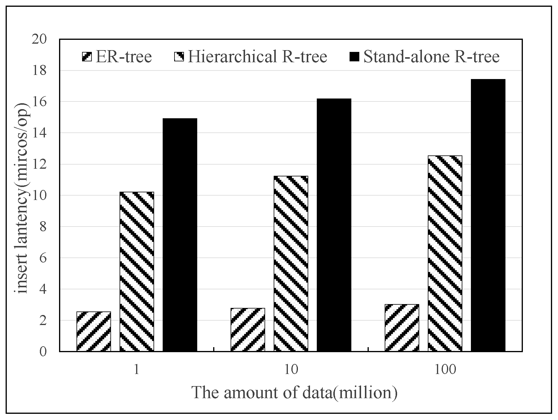
In this paper, the same randomly generated spatial data were inserted into the ER-tree index database, hierarchical R-tree index database and the stand-alone R-tree index database and the insertion data time was measured. The experiments were divided into three groups with 1 million, 10 million and 100 million data items and the insertion latency is defined below:
The experimental results in Figure 11 show that the insertion process of the ER-tree index has lower insertion latency than the other two. This is because the data of the stand-alone R-tree index and the hierarchical R-tree index are time-consuming to insert due to the huge index tree, resulting in lower build performance than ER-tree indexes. ER-tree indexes reduce the size of the index tree by building on the SSTable, thus decreasing the index building time.
5.2.2. ER-Tree Index Query Performance
Simulated dataset point query: For each database with different amounts of data after building the index, this paper performed 1000 random point queries and calculated the average query time to compare the query performance of the index. The experimental results are shown in Figure 12. Note that the vertical coordinate is the logarithmic axis. The results show that the ER-tree index has better point query performance than the other two. This is because ER-tree indexes are queried only once, while the other two indexes are queried twice.
Simulated dataset range query: For each database with different amounts of data after building the index, this paper performed 1000 random range queries with various range lengths and calculated the average query time to compare the query performance of the index. The experimental results are shown in Figure 13. The vertical coordinate is the logarithmic axis. The results show that the ER-tree index has better range query performance than the other two, for the same reason as the point query.
Simulated dataset circle query: For each database with different amounts of data after building the index, this paper performed 1000 random circle queries with various query radii and calculated the average query time to compare the query performance of the index. The experimental results are shown in Figure 14. The vertical coordinate is the logarithmic axis. The result shows that the ER-tree index has better circle query performance than the other two, for the same reason as the point query.
Real dataset point query: In this paper, we randomly selected a query point on the real dataset for querying and repeated the above operation 1000 times to calculate the average query time. The experimental results are shown in Figure 15. The ER-tree index shows better point query performance on both real datasets, indicating that the index design in this paper is effective.
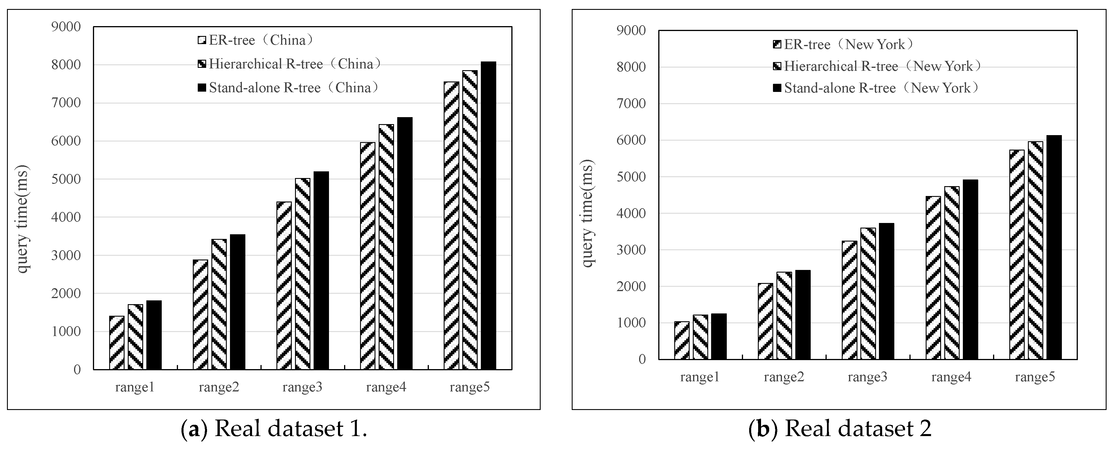
Real dataset range query: Using the centre point of the real dataset to gradually expand the query range outward, this paper conducted five range query operations on the Chinese and New York datasets, respectively and the last query covered all the data points of the real dataset. For example, the approximate centre point of New York is 75° W, 42.5° N, so the first range is from 74° W, 42° N to 76° W, 43° N and the last range is from 70° W, 40° N to 80° W, 45° N, which is roughly the entire range of New York. The experimental results are shown in Figure 16. The ER-tree index has better range query performance regardless of the range of the real dataset, indicating that the index design in this paper is suitable for both short- and large-range queries.
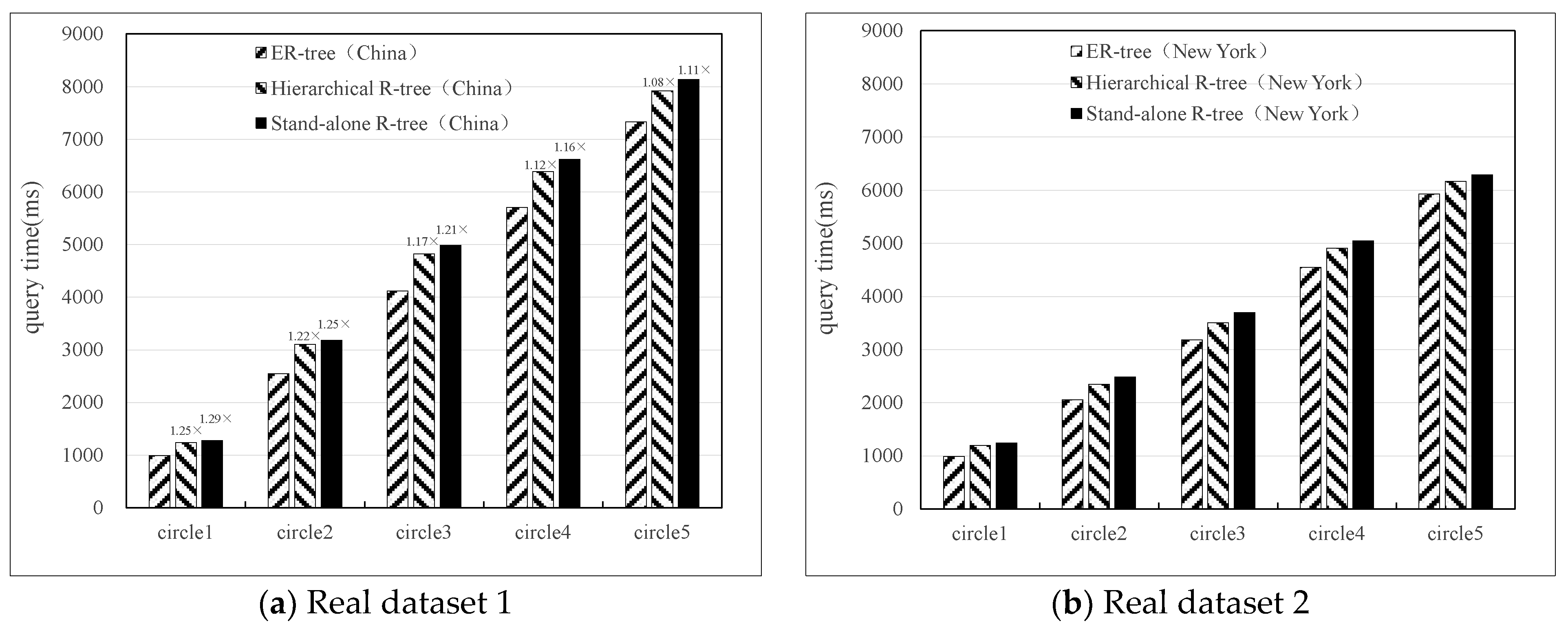
Real dataset circle query: Using the centre point of the real dataset to gradually expand the circle range outward, this paper conducted five circle query operations on the Chinese and New York datasets, respectively, and the last query covered all the data points of the real dataset. The experimental results are shown in Figure 17. Similar to the range queries, the ER-tree indexes have better query performance for both short and large circular ranges. It is worth noting that circular range queries can be used for KNN queries that are common in spatial queries.
5.2.3. ER-Tree Index Space Performance
For databases with different data volumes after building the index, this paper compared the size of the ER-tree index database file with that of a stand-alone R-tree index database file to study the space performance of the two indexes.
It can be found from the experimental results in Figure 18 that the space performance of the ER-tree index is slightly better than that of the stand-alone R-tree index. This is because the building of the ER-tree index is bottom-up, which is compacted in the storage of tree nodes and there is almost no space to waste. The stand-alone R-tree index is built from the root node to the bottom, inevitably wasting space on the node. Therefore, compared to the two indexes, the space performance of the ER-tree index is slightly better than that of the stand-alone R-tree index.
6. Conclusions
To address the problems of a low query efficiency and the dual queries of stand-alone R-tree index for spatial data on an LSM-tree, this paper designed a new ER-tree index structure based on the orderliness of an LSM-tree and optimised the dual queries into single query to improve the query efficiency of spatial data. The experiments proved that the ER-tree index was improved in the index building and the index query performance compared to the stand-alone R-tree index, and there was almost no degradation in the space performance.
Author Contributions
Data curation, J.H.; formal analysis, J.H.; investigation, J.H.; resources, H.C.; software, J.H.; writing—original draft preparation, J.H.; writing—review and editing, J.H. and H.C.; visualisation, J.H. All authors have read and agreed to the published version of the manuscript.
Funding
This research received no external funding.
Institutional Review Board Statement
Not applicable.
Informed Consent Statement
Not applicable.
Data Availability Statement
Not applicable.
Conflicts of Interest
The authors declare no conflict of interest.
References
- O’Neil, P.; Cheng, E.; Gawlick, D.; O’Neil, E. The log-structured merge-tree (LSM-tree). Acta Inform. 1996, 33, 351–385. [Google Scholar] [CrossRef]
- Chang, F.; Dean, J.; Ghemawat, S.; Hsieh, W.C.; Wallach, D.A.; Burrows, M.; Chandra, T.; Fikes, A.; Gruber, R.E. Bigtable: A distributed storage system for structured data. ACM Trans. Comput. Syst. TOCS 2008, 26, 1–26. [Google Scholar] [CrossRef]
- Ghemawat, S.; Dean, J. LevelDB. Available online: http://code.google.com/p/leveldb (accessed on 15 February 2022).
- Apache. Apache HBase: The Hadoop Database, a Distributed, Scalable, Big Data Store. Available online: https://hbase.apache.org/ (accessed on 15 February 2022).
- Alsubaiee, S.; Altowim, Y.; Altwaijry, H.; Behm, A.; Borkar, V.; Bu, Y.; Carey, M.; Cetindil, I.; Cheelangi, M.; Faraaz, K.; et al. AsterixDB: A scalable, open-source BDMS. Proc. VLDB Endow. 2014, 7, 1905–1916. [Google Scholar] [CrossRef]
- Team Facebook RocksDB. A Persistent Key-Value Store for Fast Storage Environments. Available online: https://rocksdb.org (accessed on 15 February 2022).
- Lakshman, A.; Malik, P. Cassandra: A decentralised structured storage system. SIGOPS Oper. Syst. Rev. 2010, 44, 35–40. [Google Scholar] [CrossRef]
- Lawder, J.K. The Application of Space-Filling Curves to the Storage and Retrieval of Multi-Dimensional Data. Ph.D. Dissertation, University of London, London, UK, 2000. [Google Scholar]
- Mao, Q.; Qader, M.A.; Hristidis, V. Comprehensive comparison of LSM architectures for spatial data. In Proceedings of the 2020 IEEE International Conference on Big Data (Big Data), Atlanta, GA, USA, 10–13 December 2020; pp. 455–460. [Google Scholar] [CrossRef]
- Xu, R.; Zhou, X.; Liu, Z.; Hu, H. Implementation of LevelDB-based secondary index on two-dimensional data. Journal of East China Normal University. Nat. Sci. 2019, 5, 159–167. [Google Scholar] [CrossRef]
- Xu, R.; Liu, Z.; Hu, H.; Qian, W.; Zhou, A. An efficient secondary index for spatial data based on LevelDB. In Proceedings of the International Conference on Database Systems for Advanced Applications, DASFAA 2020, Jeju, Korea, 24–27 September 2020; pp. 750–754. [Google Scholar] [CrossRef]
- Alsubaiee, S.; Behm, A.; Borkar, V.; Heilbron, Z.; Kim, Y.; Carey, M.J.; Dreseler, M.; Li, C. Storage management in AsterixDB. Proc. VLDB Endow. 2014, 7, 841–852. [Google Scholar] [CrossRef] [Green Version]
- Bozhi, Q. Research on Linked Spatial Index Based on LSM-Tree. Master’s Thesis, Zhejiang University, Hangzhou, China, 2020. [Google Scholar]
- Wang, Y.; Wu, S.; Mao, R. Towards read-intensive key-value stores with tidal structure based on LSM-tree. In Proceedings of the 2020 25th Asia and South Pacific Design Automation Conference (ASP-DAC), Beijing, China, 13–16 January 2020; pp. 307–312. [Google Scholar] [CrossRef]
- Cheng, W.; Guo, T.; Zeng, L.; Wang, Y.; Nagel, L.; Süß, T.; Brinkmann, A. Improving LSM-trie performance by parallel search. Softw. Pract. Exp. 2020, 50, 1952–1965. [Google Scholar] [CrossRef]
- Luo, C.; Carey, M.J. Efficient data ingestion and query processing for LSM-based storage systems. Proc. VLDB Endow. 2019, 12, 531–543. [Google Scholar] [CrossRef] [Green Version]
- Luo, C.; Carey, M.J. LSM-based storage techniques: A survey. VLDB J. 2020, 29, 393–418. [Google Scholar] [CrossRef] [Green Version]
- Sears, R.; Ramakrishnan, R. BLSM: A general purpose log-structured merge tree. In Proceedings of the 2012 ACM SIGMOD International Conference on Management of Data (SIGMOD ‘12), New York, NY, USA, 20–24 May 2012; pp. 217–228. [Google Scholar] [CrossRef]
- Guttman, A. R-trees: A dynamic index structure for spatial searching. In Proceedings of the 1984 ACM SIGMOD International Conference on Management of Data (SIGMOD ’84), Boston, MA, USA, 18–21 June 1984; pp. 47–57. [Google Scholar] [CrossRef]
- Kim, Y.; Kim, T.; Carey, M.J.; Li, C. A Comparative Study of Log-Structured Merge-Tree-Based Spatial Indexes for Big Data. In Proceedings of the 2017 IEEE 33rd International Conference on Data Engineering (ICDE), San Diego, CA, USA, 19–22 April 2017; pp. 147–150. [Google Scholar] [CrossRef]
- Silva, Y.N.; Xiong, X.; Aref, W.G. The RUM-tree: Supporting frequent updates in R-trees using memos. VLDB J. 2009, 18, 719–738. [Google Scholar] [CrossRef]
- Shin, J.; Wang, J.; Aref, W.G. The LSM RUM Tree: A Log-Structured Merge R-Tree for Update-intensive Spatial Workloads. In Proceedings of the 2021 IEEE 37th International Conference on Data Engineering (ICDE), Chania, Greece, 19–22 April 2021; pp. 2285–2290. [Google Scholar] [CrossRef]
- Li, F.; Lu, Y.; Yang, Z.; Shu, J. SineKV: Decoupled Secondary Indexing for LSM-based Key-Value Stores. In Proceedings of the 2020 IEEE 40th International Conference on Distributed Computing Systems (ICDCS), Singapore, 29 November–1 December 2020; pp. 1112–1122. [Google Scholar] [CrossRef]
- Lu, L.; Pillai, T.S.; Gopalakrishnan, H.; Arpaci-Dusseau, A.C.; Arpaci-Dusseau, R.H. WiscKey: Separating Keys from Values in SSD-Conscious Storage. ACM Trans. Storage 2017, 13, 1–28. [Google Scholar] [CrossRef] [Green Version]
- OpenStreetMap Contributors. OpenStreetMap Data. Available online: https://www.openstreetmap.org (accessed on 15 February 2022).
Figure 1.
Basic structure of an LSM-tree.

Figure 2.
Stand-alone R-tree indexes on LSM-trees.

Figure 3.
SSTable structure.

Figure 4.
Hilbert R-tree and R-tree comparison: (a) Hilbert curve in spatial coordinates; (b) MBR of the Hilbert R-tree; (c) MBR of the R-tree.
Figure 4.
Hilbert R-tree and R-tree comparison: (a) Hilbert curve in spatial coordinates; (b) MBR of the Hilbert R-tree; (c) MBR of the R-tree.

Figure 5.
SER-tree index structure on an SSTable.

Figure 6.
ER-tree index structure for spatial data on LSM-trees.

Figure 7.
Stand-alone R-tree index query flow.

Figure 8.
ER-tree index query flow.

Figure 9.
Circle query to the rectangular range query.

Figure 10.
Experimental data display.

Figure 11.
Comparison of the index insertion latency on the simulated datasets.

Figure 12.
Comparison of the index point query performance on the simulated datasets.

Figure 13.
Comparison of the index range query performance on the simulated dataset.

Figure 14.
Comparison of the index circle query performance on the simulated dataset.

Figure 15.
Comparison of the index point query performance on the real dataset.

Figure 16.
Comparison of the index range query performance on the real dataset.

Figure 17.
Comparison of the index circle query performance on the real dataset.

Figure 18.
Comparison of index space.

Publisher’s Note: MDPI stays neutral with regard to jurisdictional claims in published maps and institutional affiliations. |
© 2022 by the authors. Licensee MDPI, Basel, Switzerland. This article is an open access article distributed under the terms and conditions of the Creative Commons Attribution (CC BY) license (https://creativecommons.org/licenses/by/4.0/).
Share and Cite
MDPI and ACS Style
He, J.; Chen, H. An LSM-Tree Index for Spatial Data. Algorithms 2022, 15, 113. https://0-doi-org.brum.beds.ac.uk/10.3390/a15040113
AMA Style
He J, Chen H. An LSM-Tree Index for Spatial Data. Algorithms. 2022; 15(4):113. https://0-doi-org.brum.beds.ac.uk/10.3390/a15040113
Chicago/Turabian StyleHe, Junjun, and Huahui Chen. 2022. "An LSM-Tree Index for Spatial Data" Algorithms 15, no. 4: 113. https://0-doi-org.brum.beds.ac.uk/10.3390/a15040113
Note that from the first issue of 2016, this journal uses article numbers instead of page numbers. See further details here.