
Topology Optimisation under Uncertainties with Neural Networks

1
Weierstrass Institute for Applied Analysis and Stochastics, 10117 Berlin, Germany
2
Department of Mathematics, Technical University Berlin, 10623 Berlin, Germany
3
Rafinex Ltd., Great Haseley OX44 7JQ, UK
*
Author to whom correspondence should be addressed.
†
These authors contributed equally to this work.
Algorithms 2022, 15(7), 241; https://0-doi-org.brum.beds.ac.uk/10.3390/a15070241
Submission received: 13 June 2022
/
Revised: 5 July 2022
/
Accepted: 6 July 2022
/
Published: 12 July 2022
(This article belongs to the Special Issue Stochastic Algorithms and Their Applications)
Abstract
:Topology optimisation is a mathematical approach relevant to different engineering problems where the distribution of material in a defined domain is distributed in some optimal way, subject to a predefined cost function representing desired (e.g., mechanical) properties and constraints. The computation of such an optimal distribution depends on the numerical solution of some physical model (in our case linear elasticity) and robustness is achieved by introducing uncertainties into the model data, namely the forces acting on the structure and variations of the material stiffness, rendering the task high-dimensional and computationally expensive. To alleviate this computational burden, we develop two neural network architectures (NN) that are capable of predicting the gradient step of the optimisation procedure. Since state-of-the-art methods use adaptive mesh refinement, the neural networks are designed to use a sufficiently fine reference mesh such that only one training phase of the neural network suffices. As a first architecture, a convolutional neural network is adapted to the task. To include sequential information of the optimisation process, a recurrent neural network is constructed as a second architecture. A common 2D bridge benchmark is used to illustrate the performance of the proposed architectures. It is observed that the NN prediction of the gradient step clearly outperforms the classical optimisation method, in particular since larger iteration steps become viable.
Keywords:
topology optimisation; deep neural networks; model uncertainties; random fields; convolutional neural networks; recurrent neural networksMSC:
35R60; 47B80; 60H35; 65C20; 65N22; 65J101. Introduction
Structural topology optimisation is the (engineering-oriented) process of designing a construction part using optimisation algorithms under certain constraints. The resulting designs usually have a large influence on the subsequent production costs. The starting point of the process is a design domain that represents the maximum space available for the optimised component to be developed. The outcome presents information about which parts of the design space are occupied by material and which are void. Often, the task is motivated by mechanical requirements, e.g., sufficient stiffness of the constructed part with respect to assumed forces acting on it while certain predetermined points or surfaces should connect to other parts. A typical physical model for this comes from linear elasticity, describing the displacement field given material properties and forces. For the mathematical optimisation, it is repeatedly necessary to compute the stress distribution determined by the physical model in the design domain (more precisely, in the parts of the domain with material). This potentially complex computational task usually relies on the finite element method (FEM), which is based on a discretisation of the domain into elements. Most commonly, the domain is represented as mesh consisting of disjoint simplices, i.e., triangles in 2D and tetrahedra in 3D.
Since the optimisation process easily requires several hundred evaluations of the state equation to evolve the material distribution, it is of significant interest to develop techniques that reduce this computational burden. This becomes much more pronounced when uncertainties of the model data should be considered in the computations. The treatment of uncertainties has been developed extensively from a theoretical and practical point of view over the last decade in the area of Uncertainty Quantification (UQ). A common way to describe uncertainties is by means of random fields, whose (Karhunen-Loève) expansions depend on a possibly very large number of random variables. The parameter space spanned by these random variables leads to very high-dimensional state problems for which the derived optimisation problems are very difficult to solve.
This paper investigates the application of a trend in scientific computing for current topology optimisation methods, namely the use of modern machine learning techniques. More precisely, our objective is to improve the efficiency of the structural topology optimisation problem by predicting gradient steps based on generated training data. This efficiency gain directly transfers to our ability to compute much more involved risk-averse stochastic topology optimisation problems with random data. In this case, the topology is optimised with an adjusted cost functional including the CVaR (conditional value at risk), by which unlikely events can be taken into account in contrast to simply optimising with the mean value of possible load scenarios. In addition to random loads, we also include random material properties which, e.g., can enter the model in terms of material errors or impurities. We emphasise that risk-averse optimisation based on some risk measure is a timely topic, which plays a role in many application areas. Despite its relevance, this type of problem has not been covered widely in the literature yet. In fact, the authors are not aware of any other machine-learning-assisted approach for risk-averse topology optimisation. This might be due to the more involved mathematical framework and substantially higher computational complexity. To achieve performance benefits with topology optimisation in this paper, we adapt concepts from the field of deep learning to approximate multiple iterations of the optimisation process and render the overall optimisation more efficient.
The goal of topology optimisation is to satisfy the technical requirements of a component (for instance, stiffness with respect to certain loading scenarios) with minimal use of material. There are different approaches to describe the topology in a flexible way such that substantial changes are possible. We follow our previous work in [1] and use a phase field model which describes the density of material with a value in . The starting point is the definition of a physical design space available for the component under consideration. This space is completely filled with a material in the sense of an initial solution. Furthermore, all points at which loads act on the component, as well as the type of the respective load, are prescribed. The optimisation aims to achieve a homogeneous, minimum possible deformation at all optimised points of the component under the imposed (possibly continuous and thus infinitely many) loading scenarios. Here, a minimum compliance corresponds to a maximum stiffness. In general, even solving the underlying partial differential equation (PDE) of this problem for deterministic coefficients of the PDE presents a complex task. Furthermore, PDE coefficients which describe material and the loads have a strong influence on the resulting topology, i.e., even small changes in these coefficients can lead to large differences in the resulting topology. This results in considerable computational effort in the stochastic settings, since the solution has to be calculated for a sufficient number of data realisations to become reliable. Hence, the modelling of these stochastic settings for example (with the most obvious approach) by a Monte Carlo (MC) simulation increases the required iteration steps linearly in the number of simulations.
A method to numerically tackle topology optimisation uncertainty was presented in [2]. In this paper, we extend the previous work by introducing Deep Neuronal Networks (DNN) that are designed to provide a prediction of the next gradient step. Since topologies discretised with finite elements can be represented as images, Convolutional Neural Networks (CNN) seem natural candidate architectures for this task and there has already been some research on this approach for the deterministic setting. An introduction is presented in [3] where the conventional topology optimisation algorithms are replicated in a computationally inexpensive way. Furthermore, a CNN is used in [4] to approximate the last iteration steps of a gradient method of a topology optimisation after a fixed number of steps to refine a “fuzzy” solution. A CNN architecture is also used in [5] to solve a topology optimisation problem and trained with large amounts of data. The resulting NNs were able to solve problems with boundary conditions different to their training data. In [6], the problem is stated as an image segmentation task and a deep NN with encoder–decoder architecture is leveraged for pixel-wise labeling of the predicted topology. Another encoding–decoding U-Net CNN architecture is presented in [7], providing up- and down-sampling operators based on training with large datasets. In [8] a multilevel topology optimisation is considered where the macroscale elastic structure is optimised subject to spatially varying microscale metamaterials. Instead of density, the parameters of the micromaterial are optimised in the iteration, using a single-layer feedforward Gaussian basis function network as surrogate model for the elastic response of the microscale material.
A discussion on solving PDEs with the help of Neural Networks (NN) for instance of the Poisson equation and the steady Navier–Stokes equations is provided in [9]. In a relatively new approach, through a combination of Deep Learning and conventional topology optimisation, the Solid Isotropic Material with Penalisation (SIMP) was presented in [10], which could reduce the computational time compared to the classical approach. The authors use a similar method as [4] except that the underlying optimisation algorithm performs a mesh refinement after a fixed number of iterations. To improve this step, separately trained NNs are applied to the respective mesh in order to approximate the last steps of the optimisation on the corresponding mesh. The result is then projected to the next finer mesh and the procedure is repeated a fixed number of times. A SIMP density field topology optimisation is directly performed in [11]. The problem can be represented in terms of the NN activation function. Different beam problems comparable to our experiments are depicted. Fully connected DNNs are used in [12] to represent implicit level set function describing the topology. For optimisation, a system of parameterised ODEs is used. A two-stage NN architecture which by construction reduces the problem of structural disconnections is developed in [13]. Deep generative models for topology optimisation problems with varying design constraints and data scenarios are explored in [14]. In [15], direct predictions without any iteration scheme and also the nonlinear elastic setting are considered. Examples are only shown for a coarse mesh discretisation of the design domain. In [16], an NN-assisted design method for topology optimisation is devised, which does not require any optimised data. A predictor NN provides the designs on the basis of boundary conditions and degree of filling as input data for which no optimisation training data are required.
The main goal of this paper is to devise new NN architectures that lower the computational burden of structural topology optimisation based on a continuous phase-field description of the density in the design domain. In particular, the approach should be able to cope with adaptive mesh refinements during the optimisation process, which has shown to significantly improve the performance of the optimisation. Moreover, as a consequence of an efficient computation in a deterministic setting, a goal is to transfer the developed techniques to the stochastic setting for the risk-averse topology optimisation task. The general strategy is to combine conventional topology optimisation methods and NNs in order to reduce the number of required iteration steps within the optimisation procedure, increasing the overall performance.
The main achievements of this paper are two new NN architectures that are demonstrated to yield state-of-the-art numerical results with a much lower number of iterations than with a classical optimisation. Moreover, in contrast to several other works that are solely founded on the image level of topology, our architectures make use of a very versatile functional phase-field description of the material distribution, which we have not observed in the literature with regard to NNs. This also holds true for the stochastic risk-averse framework, which to our knowledge has not been considered with NN predictions yet. Another novelty is the mixture of a fine reference mesh and adaptive iteration meshes during optimisation.
Inspired by the work of [5,10], as a first new NN architecture we develop a new CNN approach and show that it can replicate the reference results of [1,2]. In contrast to [10], we only have to train one NN for the entire optimisation despite mesh refinement being carried out in the iterative procedure. We subsequently extend this approach to the stochastic setting with risk-averse optimisation from [2]. Based on the CNN, we further extend the optimisation with a Long Short-Term Memory (LSTM) architecture as a second novel method. It encodes the change of the topology over several iteration steps, thus resulting in a more accurate prediction of the next gradient step.
In the numerical experiments, it can be observed that the two presented architectures perform equally well as our reference implementation. However, fewer iteration steps are required (i.e., larger steps can be used) since the gradient step predictions seem to be better than when computed with a classical optimisation algorithm.
The structure of the paper is as follows. In Section 2, we introduce the underlying setting from [1,2] and discuss the algorithms used for phase-field-based topology optimisation. In this context, we introduce the linear elasticity model and derive a state equation, the adjoint equation and a gradient equation, whose joint solution constitutes the optimisation problem under consideration. In Section 3, we present two different architectures of the NNs approximating multiple steps of the gradient equation. We start with a CNN that is well suited for processing the discretised solutions of the equations from Section 2. This is then extended to a long short-term memory NN, which is able to process a sequence of these solutions simultaneously and thus achieves a higher prediction quality. Since the data of the finite element simulation do not directly match the required structure of NNs, we provide a discussion of the data preparation for both architectures. Section 4 illustrates the practical performance of the developed NN architectures with a standard benchmark (a 2D bridge problem). The work ends with a summary and discussion of the results and some ideas for further research in Section 5. The appendix provides some background on the used problem, in particular the standard benchmark problem in Appendix A and the finite element discretisation in Appendix B. The implementation and codes for the generation of graphics and data to reproduce this work are publicly available (https://github.com/MarvinHaa/DeepNNforTopoOptisation accessed at 1 June 2022).
2. Topology Optimisation under Uncertainties
We are concerned with the task of topology optimisation with respect to a state equation of linear elasticity. This problem becomes more involved when stochastic data are assumed. In our case, this concerns material properties and the forces acting on the designed structure. These translate into the engineering world as material imperfections or fluctuations and natural forces such as wind or ocean waves. Such random phenomena are modelled in terms of random fields that often are assumed to be Gaussian with certain mean and covariance.
It is instructive to first present the deterministic topology optimisation task, which we discuss in the following Section 2.1. Subsequently, in Section 2.2 we extend the model to exhibit random data, allowing an extension of the cost functional to also include the fluctuations of the data in terms of a risk measure. In our case, this is the so-called conditional value at risk (CVaR).
For the sake of a self-contained presentation, we provide all equations that lead to the actual optimisation problem, which is given in terms of a gradient that evolves a phase field. Thus, the entire problem formulation can be understood and the required extensions to obtain the risk-averse formulation become clear. However, in case the reader is only interested in the proposed NN architectures, it might be sufficient to simply gloss over the most important parts of the problem definition, for which we provide a guideline as follows: The linear state equation is given in Equation (1), leading to the weak form in Equation (2) that is used for the computation of finite element solutions. These are required in the deterministic minimisation problem given in Equation (4), which is solved iteratively by computing the gradient step defined by Equation (6). A similar problem formulation, extended by an approximation of the CVaR risk measure, can be obtained in case of the risk-averse optimisation. This is given in Equation (9) and can be solved iteratively with gradient steps defined by Equation (11).
The presentation of this section is based on [1,2] where the optimisation problem computes the distribution of material in a given design domain described by a continuous phase field depending on the realisation of the random parameters. The optimum of this problem maximises stiffness while minimising the volume of material for the given data.
2.1. Deterministic Model Formulation
The goal is to determine an optimal distribution of a material (with density or probability) in a compact design domain . We further assume that D satisfies sufficient regularity assumptions such that the PDE state equation exhibits a unique solution. The desired optimality of the task means that the resulting topology is as resilient (or stiff) as possible with respect to the deformation caused by the expected forces acting on it, which are described by a differentiable vector field .
Definition 1.
The distribution of a material in is represented by a phase field with for all , where if there is material at position x and if there is no material at position x. At the phase transitions we allow to ensure sufficient smoothness for phase shift. We call the evaluation of φ topology.
Note that the actual topology is reconstructed in a post-processing step by choosing some threshold in to fix the interface between material and void phase of the phase field.
2.1.1. Linear Elasticity Model
The state equation corresponding to the above problem is described by the standard linear elasticity model [17]. To define the material tensor, we first define the strain displacement (or strain tensor) by
which specifies the displacement of the medium in the vicinity of position x. Moreover, a so-called blend function is given by
ensuring a smooth transition between the phases. According to Hooke’s law and by using the Lamé coefficients and , the isotropic material tensor for the solid phase is given by
This material tensor describes the acting forces between adjacent positions in the connected material, where and are two material parameters characterising the strain–stress relationship. For the void phase, to ensure solvability of the state equation in entire domain D, we define the tensor as a fraction of the material phases. More precisely, we set with some small . Hence, the material tensor (or stress tensor) is given by
Using the material tensor , a force with load (a pressure field) and the phase field , the displacement vector field u is described by the state equation of the standard linear elasticity model given by
This implies that on boundary subspace the material is fixed while on the force g acts on the material. On the boundary the material is barred from movement in normal direction n. In the following, equality is to be generally understood in a pointwise manner.
2.1.2. State Equation
The weak formulation of the state Equation (1) can be formulated as: find such that
where is the usual Sobolev space and the Lebesgue measure and
and
These definitions are in particular used for the finite element discretisation described in Appendix B.
2.1.3. Adjoint Equation
To define the optimisation problem, we introduce the Ginsburg–Landau functional , which serves as a penalty term for undesired variations and is defined by
where is the Euclidean norm. This ensures that the solution to the optimisation problem can be interpreted as an actual smooth shape. The double well functional with penalises values of that differ from 0 or 1 and the leading term limits the changes of . This results in the cost functional to be minimised,
The adaptivity parameter controls the weight of the interface penalty and hence has a direct influence on the minimum respective to the characteristics of the resulting shape of . In fact, is chosen adaptively to avoid non-physical or highly porous topologies, see [2]. Additionally, we require the volume constraint with to limit the amount of overall material.
The (displacement) state u from Equation (3) is obtained by solving the state Equation (2), which is used in the optimisation problem
The Allen–Cahn gradient flow approach is used to determine the solution for which the adjoint problem of Equation (4) is used to avoid the otherwise more costly calculation. It is shown in [2] that for the corresponding adjoint problem can be formulated as: find such that
which is identical to the state equation. Hence, the respective adjoint solution p is equal to the solution u of Equation (2) and no additional system has to be solved.
2.1.4. Gradient Equation
With the solutions u respective to p one gradient step with adaptive step size can be characterised by the unique solution such that, for all ,
The restriction on for all is realised by in every iteration step. For the calculation of the minimum of Equation (4), the state Equation (1), the adjoint Equation (5) and subsequently the gradient Equation (6) are solved iteratively until converges. We always assume that solutions u and exist, which in fact can be observed numerically. The proposed procedure is described by Algorithm A1 where the solution of the integral equations takes place on a discretisation of D. The algorithm solves the state, adjoint and gradient equations in a loop until the solutions of the gradient equations only change slightly. The discretisation mesh is subsequently refined and the iterative process is restarted on this adjusted discretisation.
2.2. Stochastic Model Formulation
In the stochastic setting, the Lamé coefficients (determining the material properties) and and the load scenarios are treated as random variables on some probability space . The randomness of the data is inherited by the solution of the state equation as well as the adjoint equation. As a result, the gradient step can be considered as a random distribution, see again [1,2]. The goal is to minimise the functional for the expected value of as well as for particularly unlikely events. For the formulation of an adequate risk-averse cost functional, we introduce the conditional value at risk (CVaR). The CVaR, a common quantity in financial mathematics, is defined for a random variable X by
with and . It characterises the expectation of the -tail quantile distribution of X, hence accounting for bad outliers that may occur with low probability. The stochastic state equation can be formulated analogously to Equation (5) in the deterministic setting.
2.2.1. Adjoint Equation
For the risk-aware version of Equation (3) with respect to the CVaR parameter , we define the cost by
In the special case , the CVaR is nothing else than the mean, i.e.,
This results in the stochastic minimisation problem analogous to Equation (4) given by
Following [2], the CVaR can be approximated in terms of the plus function. The solution of Equation (8) can hence be rewritten as
An obvious approach to solve this optimisation problem is a Monte Carlo simulation, i.e., for each iteration step with evaluation of , state Equation (1) have to be solved for different parameter realisations. The associated adjoint problem to Equation (9) reads
Consequently, the solution of Equation (10) is given by
2.2.2. Gradient Equation
Analogous to the deterministic approach, the gradient can be defined corresponding to Equation (9) by the solution , such that for all the following equation holds,
The actual solution for one gradient step of the minimisation problem in Equation (8) with respect to (9) follows from
where is the number of samples of the Monte Carlo simulation. The larger chosen, the larger t becomes, and thus the number of evaluations of u for which holds true increases. In order to ensure a valid simulation of Equation (12), N must be chosen sufficiently large so that an adequate number of evaluations of u in each gradient step fulfils condition . The described procedure is depicted in Algorithm A2 where the optimisation process is basically the same as in Algorithm A1. The central difference is that realisations of the optimisation problem have to be computed in each iteration. In practice, these are solved in parallel for N different and the results are then averaged. The large computational efforts caused by the slow Monte Carlo convergence are alleviated by the neural-network-based machine learning approaches presented in Section 3. In particular, gradient steps for arbitrary parameter realisations can be evaluated very efficiently and significantly fewer iterations (i.e., optimisation iterations) are required.
3. Neural Network Architectures
In modern scientific and engineering computing, machine learning techniques have become indispensable in recent years. The central goal of this work is to devise neural network architectures to facilitate an efficient computation of the risk-averse stochastic topology optimisation task. In this section, we develop two such architectures. The first one described in Section 3.1 is based on the popular convolutional neural networks (CNN) that were originally designed for the treatment of image data. In Section 3.2, a classical long short-term memory architecture (LSTM) is adapted to predict the gradient step.
The usage of deep neural networks with topology optimisation tasks have been previously examined in [4,10]. However, in contrast to other approaches, our architecture aims at a single NN that can be trained to handle arbitrarily fine meshes in terms of the requirements warranted during the topology optimisation process. More precisely, we seek an NN that predicts the gradient step from Equation (6) discretised on an arbitrarily fine mesh at an arbitrary iteration step with given , for such that
Thus, the total number of iterations required for the topology optimisation iteration should ideally be reduced, resulting in improved practical performance. For the sake of a convenient presentation, we consider all other coefficients of Equation (6) as constant in the following analyses. Alternatively, one would have to increase the complexity in the number of degrees of freedom which are the weights describing the NN as well as the required training data. It can be assumed that with more information in the form of coefficients provided to the NN during training the accuracy of the resulting approximation of increases. Within the optimisation procedure, the actual calculation of the gradient step given in Equation (6) is performed on the basis of variable coefficients (e.g., and ).
Since the discretisation can be rewritten rather easily in tensor form, which represents the input of a CNN, this is the first architecture we consider in the next section.
3.1. Topology Convolutional Neural Networks (TCNN)
When using a visual representation of topologies as images (as they can be generated as output of a finite element simulation), the solution of Equation (6) can be easily transferred to the data structures used in CNNs. Consequently, predicting the gradient step with a CNN can be understood as a projection of the optimisation problem into a pixel-structured image classification problem. Here we assume that the calculation of the learned gradient step is encoded in the weights that characterise the NN.
In principle, the structure of a classical CNN consists of one or more convolutional layers followed by a pooling layer. This basic processing unit can repeat itself as often as desired. If there are at least three repetitions, we speak of a deep CNN and a deep learning architecture. In the convolutional layers a convolution matrix is applied to the input. The pooling layers are to be understood as a dimensional reduction of their input. Although common for image classification tasks, pooling layers are not used in the presented architecture.
3.1.1. TCNN Architecture
We follow the presentation of the pytorch documentation [18]. The input of a layer of the CNN architecture is a tensor . Here, is the number of input samples, in our case the evaluations of and u as presented in Section 3.1.2. It is therefore possible to calculate the gradient step from Equation (6) for several different loads g simultaneously. This way, Monte Carlo estimates become very efficient. corresponds to the number of input channels and each channel represents one dimension of an input ( or u). and provide information about the dimension of the discretisation of the space D. The output of one CNN layer is specified by . For fixed and with the number of output channels is given as
Here, * denotes the cross-correlation operator, and with is a cutout of . The weight tensor determines the dimensions of the kernel (or convolution matrix) of the layers with .
For simplicity, we henceforth assume unless otherwise specified. In particular, the entries of the weight tensor are parameters that are optimised during the training of the CNN. Depending on the architecture of the CNN, an activation function evaluated element-wise can additionally be applied to Equation (14).
Definition 2.
Let and with be given by one parameter vector with
Furthermore, let σ be a continuously differentiable activation function. We call a function
a convolution layer with activation function σ if it satisfies
with .
A sequential coupling of this layer structure provides the framework for the CNN. Specifically, for ,
Definition 3
(CNN architecture). Let , for and for with be given by some parameter vector with
Furthermore, let be given continuously differentiable activation functions. We call an NN of the form of Equation (17) an L-layer topology convolutional neural network (TCNN) and characterise it as the mapping
The approximation of is hence determined by its parameter vector . For general CNNs, the dimension does not have to be constant across the different layers. The same holds true for the dimensions of the kernel matrices. In fact, before implementing the convolution, we embed each channel of our input in a space to preserve the dimension in the output.
Example 1.
The following specific TCNN has proved to be the most suitable for integration into Algorithm A1 for the selections of hyperparameters we have investigated. The architecture is given as an layer TCNN with input channels, for hidden channel, output channel and kernel size as well as trained weights described by which determine the mapping by
with activation function . In contrast to many standard architectures, only the activation function of the output layer is not the identity. We chose as input space in anticipation of the setting in Example 2, reflecting our mesh choice to discretise domain with nodes, which for first-order finite elements then is the dimension of the discrete functions u and φ. The architecture is depicted in Figure 1.
3.1.2. Data Preparation
On the algorithmic level, our goal is to replace the computationally costly lines 5 and 6 of all loop iterations of Algorithm A1 with a TCNN. This is not directly possible (at least for a TCNN) since the input space of a TCNN does not match the mesh on which the finite element discretisation and thus the optimisation of takes place in the current optimisation step t. Hence, it is necessary to project the evaluation of onto the format of a CNN. For this we define a transformation between and the input tensor of . As described in Appendix B, we do not assume that the mesh stays fixed in the optimisation algorithm and we instead generate a sequence of different meshes by some adaptive mesh refinement, which has led to significant efficiency improvements in [1]. To obtain unique transformations between the discretisation finite element space and the input space of the NN, one can interpolate the current solutions of and from onto a constant reference mesh by polynomial interpolations
Hence, during the optimisation, the current solutions are interpolated via the operator p to the reference mesh, rendering the prediction independent from the actual adaptive mesh. After the prediction of the gradient step on the reference mesh, it is mapped back to the actual computation mesh via q.
Consequently, we define the reference mesh with vertices V and edges E as a graph such that . Each node corresponds to the values of and at node . The features of the nodes can hence be interpreted as rows of a feature matrix,
The structure of is illustrated in Figure 2.
One can now define a transformation between and by
Hence, the approximation of the gradient step 6 of Algorithm A1 is basically a coupling of the mappings p, and , namely
Example 2
(Illustrating the TCNN). The NN given by the coupling of functions in Equation (21) with given as in Example 1 can be described by
with
for and defined on . Hence, this NN can be applied directly to the finite element discretisations and used in Algorithms A1 and A2.
With the TCNN from the example in Equation (23) we have extended Algorithm A1. More precisely, we have inserted an NN approximation in each of the steps, which predicts k iteration steps by just one evaluation. For this, the sequence has to be defined in advance. We leave it to future research to adaptively control the sequence dynamically within the optimisation algorithm. This extension of Algorithm A1 is described by Algorithm 1. In an analogous way, we also extend Algorithm A2 by the TCNN given in Equation (23). In particular, we are able to evaluate all samples in parallel by adding additional sample dimensions to the input tensor of the TCNN given in Equation (14). This procedure is illustrated in Algorithm 2. Again, the parameter has to be chosen in advance.
| Algorithm 1: Deterministic optimisation algorithm with TCNN approximated gradient step |
 |
| Algorithm 2: Stochastic optimisation algorithm with TCNN approximated gradient step |
 |
3.2. Topology Long Short-Term Memory Neural Networks (TLSTM)
One possible approach to improve the prediction of using an NN is to provide the classifier not just one tuple as an inpu, but to have it process a larger amount of information by a sequence of these tuples of the last iteration steps, i.e.,
Through this, the shift of the phase field or the change of the topology over time is also transferred as input to the NN. The sequence prediction problem considered in this case differs from the single step time prediction in the sense that the prediction target is now a sequence that contains both spatial and temporal information. Theoretically, this information can also be learned directly from the NN. However, in practice it is more effective to adapt the architecture to the information we have in advance (in our case with respect to the time dependency) to achieve better results. An NN that allows exactly this is a recurrent Neural Network (RNN). Unfortunately, standard RNNs often suffer from the vanishing gradient problem [19,20] which we try to prevent from the beginning. Therefore, we build on the special RNN concept of a Long Short-Term Memory (LSTM) in the context of our problem, which is more robust against the vanishing gradient issue and provides promising results, especially in the analysis of time series. For a background on time series analysis and a review of the different methods, we refer to the survey article [21]. In practice, time series are usually stored as one-dimensional sequences in vector format. Consequently, there is no out-of-the-box LSTM layer implementation for structures such as the input tensor we require in Equation (14). Nevertheless, we still do not wish to abandon the mechanism of convolution within the NN in order to keep the structural information of and u. An LSTM layer with a convolutional structure can be constructed by replacing the matrix vector multiplication within a standard LSTM layer by convolutional layers. The unique advantage of an LSTM according to [20] is its cell-gate architecture, which mitigates the vanishing gradient problem. More precisely, it consists of a “memory cell” that serves as an accumulator of the current state , in the processed sequence. The information capacity of the last status within is controlled by the activation of the so-called “forget gate” . The information capacity of the input state is controlled by the activation of the input gate . Which information (or whether any at all) gets transferred from memory cell to state is in turn controlled by the activation of the output gate . From a technical point of view, the gates can be understood as learning forward layers.
3.3. TLSTM Architecture
An ordinary LSTM layer to generate complex sequences with long-range structure as presented in [22] corresponds to the described logic above and can be formulated numerically for a sequence of one-dimensional input state and output vector as an equation system
where with and tanh are evaluated element-wise. The operation ⊙ denotes the Hadamard product and the subscripts of the weight matrices describe the affiliation to the gates. For example, is the weight matrix to input of gate . This illustrates how the weights of the LSTMs are transferred to the weights of convolution LSTMs in the following.
We want to reformulate Equation (24) by replacing all matrix-vector multiplications (i.e., the forward layer) with a convolution layer from Definition 2. This is inspired by [23], which has already provided the theoretic architecture of a convolutional LSTM layer with the approach on precipitation forecasting. Let be a convolutional layer and a sequence of inputs ordered by the discrete time dimension . A convolutional LSTM layer to an input sequence and (since at we do not yet have any information about earlier steps in the sequence) is given by a system of equations,
with and the output of the convolutional LSTM layer as well as in Equation (24). The subscript t indicates a cutout of the t-th element of sequence dimension T of the respective tensor.
Definition 4
(LSTM layer). Let as well as and parameter vectors, specifying the convolutional layer as in Definition 3 for from Equation (25),
and described by the parameter vector , with
Furthermore, let with and tanh be evaluated element-wise. We call a function,
an LSTM layer, if it satisfies the mapping rule given by the system of Equation (25).
For the forecasting of our gradient sequence, we use an encoder–decoder architecture (i.e., an “autoencoder”) consisting of , LSTM layers,
that satisfies the mapping rule given by the equation system (25) with . Therefore, the encoding and decoding blocks of the autoencoder have the same number of layers . The autoencoder for an input sequence can be described by the following system of equations of the encoder block,
with . This is combined with the following decoder block by setting and and ,
with .
It should be mentioned that the input and output sequences do not have to be of the same length (in fact, in general ). Furthermore, holds for individual LSTM layers defined in Equations (26) and (27). Especially, since the output sequence is also input of , it holds that . In order to be able to select the dimensions of the output tensor completely independently of the hidden channels, we additionally apply a convolutional layer with activation function to concatenate the hidden channel to an arbitrary number of output channels given by
Definition 5
(TLSTM architecture). Let as well as , with be given. Hence, the respective LSTM layers from the encoder defined in Equation (26) and decoder in (27) block as well as the output layer in Equation (28) can be described by the parameter vectors of the CNN and LSTM layers (see Definition 3 for and Definition 4) with for and an activation function of the output layer. These parameter vectors as well as the weight tensors and for can in turn be described collectively by the parameter vector , where
We call an NN as described in Equations (26)–(28) Convolutional Topology Long Short-Term Memory (TLSTM) and characterise it by
The difference between a TLSTM and an LSTM is therefore the structure of the input tensor of a TLSTM instead of and the internal calculation carried out with convolutional layers instead of standard multiplications.
Example 3.
For the experiments in Section 4.2, the underlying layer TLSTM with input channels, hidden channels, output channel, kernel size of all included convolutional layers and sequence lengths , with trained weights described by are given as
with activation function . The autoencoder structure for an 8-layer LSTM described in Equations (26)–(28) for (29) is visualised in Figure 3.
3.4. Data Preparation
As in the case of the integration of the proposed in Section 3.1, we want to replace lines 5 and 6 in Algorithm A1 with the approximation of the from Definition 5. In case of a TLSTM, the evaluations of and u have to be transformed from the graph structure of the finite element simulation into an appropriate tensor format. This in principle is analogous to the composition in Equation (21). The only difference is that now this is performed on a sequence of evaluations and of length . As the subscripts suggest, such a sequence does not necessarily have to be evaluated on a fixed mesh , it may extend over a sequence of meshes . However, since we use polynomial interpolations
to transfer the sequence and onto some reference mesh .
We intend to process feature matrices of the form of Equation (19). Hence, we define transformations
Thus, the approximation of a gradient step in Algorithm A1 by a TLSTM can be understood as a concatenation of the form
Example 4
(The TLSTM). The NN given by the coupling of functions from Equation (31), where as given in Example 3, can be described by
and
for and defined on mesh .
The TLSTM from Example 4 can directly be integrated into Algorithm A1 as with the previous integration with Algorithm 1. In fact, since in Algorithm A1 only the most recent gradient step is relevant, in practice we restrict the inverse mapping on the last element of the predicted sequences to save calculation time. The only difference is that the sequences and have to be stored in a list. We chose and for all . This procedure is described in Algorithm 3. As in the case of the TCNN, we are able to include the extra sample dimension S to approximate gradient steps from multiple problems at once.
| Algorithm 3: Deterministic optimisation algorithm with TLSTM approximated gradient step |
 |
4. Results
This section is devoted to numerical results of the two previously described neural network architectures. The implementations were conducted with the open source packages PyTorch [18] for the NN part and FEniCS [24] for the FE simulations (see introduction for the link to the code repository). We first illustrate the performance of the TCNN in Section 4.1 with a deterministic bridge example compared to a classical optimisation. The important observation is that with the TCNN the optimisation can be carried out with far fewer optimisation steps while still leading to the reference topologies from [1]. Similar results can be observed for the risk-averse stochastic optimisation. In Section 4.2, numerical experiments of the TLSTM architecture are presented. The performance is revealed to be comparable to the TCNN architecture and the optimisation appears to be more robust with respect to the data realisations.
4.1. TCNN Examples
Before we can use the TCNN architecure for the optimisation in Algorithm 1, we have to train it on data that describe the system response of Equation (6). Note that it would not be useful to allow the to learn the gradient steps of a fixed setting since different settings of the bridge problem from Appendix A.1 should efficiently be tackled. In considering the stochastic setting of the problem as defined in Section 2.2, the TCNN is trained to learn the gradient steps for a random .
4.1.1. Sampling the Data
To train the architecture, appropriate training data have to be generated. In order to achieve this, we chose the same setting for g as in Appendix A.2. Using the optimiser in Algorithm A1, we can generate different sample paths of gradient steps and solutions of the state equation by generating S samples of g. In this procedure, we store every iteration step of and in order to approximate k gradient steps at once. More precisely, we store tuples
with , where is fixed in advance, representing the maximum number of iterations of an optimisation. For the training of the models in the following experiments, we have chosen since the topologies have mostly converged after this number of iterations. The overall number of tuples are merged into an unsorted data set .
4.1.2. TCNN Predictions
The following experiment validates that the performance of Algorithm A1 can be replicated or (desirably) improved by including a CNN as described in Algorithm 1. As a first test, we illustrate that the proposed new architecture is indeed capable of predicting the gradients of the optimisation procedure.
Figure 4 shows the evaluations of the model Equation (22) after determining within the training of the NN on the data set . Here, the prediction and the actual gradient step generated by Algorithm A1 are compared for different loads sampled from a truncated normally distributed g. Since the predictions of are hardly distinguishable from the reference fields, we have also trained Equation (22) to predict larger time steps (for 25 and 100 iteration steps at once). However, these NNs have proved to be less reliable in practice as prediction quality decreases. An illustrative selection of some predictions is provided in Figure A5 and Figure A6 in Appendix C.
4.1.3. Deterministic Bridge Optimisation
In these experiments we compare the performance of Algorithm 1 with that of Algorithm A1 in the setting of Appendix A.1. For the NN in Algorithm 1, we use Equation (22) from Example 2. For in Algorithm 1 we chose for all . In order to train Equation (22), data of the form of Equation (33) from Section 4.1.1 are used. We expect that the best (reference) results in the setting from experiment A.1 can be obtained, since the distribution of the training data is a truncated normal distribution around this expected value and we thereby have an accumulation of training points around the load . As a convergence criterion, we used the convergence criterion of the mesh refinement of Equation (A1) on a maximally fine mesh with . A sub-sequence generated by Algorithm 1 is shown in Figure A7a in comparison to that of Appendix A.1 in Figure A7b in Appendix C. There, it can be observed that the classical and CNN-assisted optimisation results essentially appear identical with the faster CNN convergence.
The metrics for evaluating our algorithms have also improved through the application of the CNN as can be observed in Figure 5. For better comparability, we ran both algorithms 10 times and averaged all metrics. To be more precise, this is only the average of the calculation time, as the remaining metrics are deterministic and therefore always the same. It is easy to see how the metrics diverge with the first application of the CNN at iteration step 55, especially by the computation time required per iteration. The most significant indicator is the evaluation of per iteration of Equation (3) at the top-right of Figure 5. The graph for Algorithm 1 reaches a constant lower level than that of Algorithm A1 after about 250 iterations and thus fulfils the convergence criterion earlier. Accordingly, the step size criterion for applies earlier by using the CNN, which further accelerates convergence. An interesting insight is provided by the calculation time, which shows that the actual time required per iteration step is more or less the same, except for the iteration steps in which Equation (22) is applied. This is indicated by the upward outliers in the computation time series. This additional computation cost can be explained by the application of the mesh projection of Equation (21), which represents an aspect requiring further improvements. Nevertheless, in total we achieve a shorter total run-time due to the faster convergence of Algorithm 1.
A detailed list of the run-times and target value metrics for the functional is provided in Table 1. The evaluation of denotes the value of the functional for the topology converged after iteration steps. The compliance is the value that is actually minimised in terms of the functional . Algorithm 1 requires less computing time than the reference procedure after extending it with the CNN architecture from Equation (22).
4.1.4. Stochastic Bridge Optimisation
Algorithm A2 can easily be extended by the TCNN of Equation (22) in order to improve the efficiency for topology optimisation under uncertainties. The corresponding procedure is shown in Algorithm 2 where we chose for all . Note that the predictions of the different realisations of for (where an evaluation are to be interpreted as transformation of an evaluation from ) are actually not executed within a loop but in parallel (lines 8–12 of Algorithm 2). This is possible because NNs are generally able to process batches of data in parallel. We have also implemented parallelisation for Algorithm A2, which is limited by the number of processor cores of the actual compute cluster. We want to compare the performance of Algorithm A2 and Algorithm 2 using the same setting as in Appendix A.2. To ensure comparable results despite stochastic parameters, we set the random seed to 42 before running both algorithms. The resulting sub-sequences of are compared side by side in Figure 6. Although the topology converges after fewer iterations with Algorithm A2, one can see that the topology resulting from Algorithm 2 has a more stable shape since the topology does not lose material to the unnecessary extra spoke. This is confirmed by the metrics in Table 2 where one can see that Algorithm 2 achieved a lower compliance after fewer iteration steps. Additionally, the optimisation of Algorithm 2 is stopped after 500 iterations to show that it achieves a better result in less time as shown in Figure 7. A notable observation is that the times of applying Equation (22) in Algorithm 2 can be identified by the spikes in the computation time of the iterations. It can be seen that despite the additional time required by the transformation in Equation (21), the calculation of a stochastic gradient step using Equation (22) is generally faster. This is due to the dynamic parallelisation that PyTorch provides when processing batches (in our case the approximation of multiple evaluations from with NNs). However, the amount of evaluations of that Algorithm A2 can process at once is limited by the number of available processors. Since the calculation time for the evaluation of an optimisation step increases with finer meshes, the evaluation of the approximation of all gradient steps at once results in a processing time advantage for the NN. It is to be expected that this time saving increases with the number of examples S.
As mentioned at the beginning of the experiment, we expect to achieve good results close to the mean of . In order to obtain a more general view of the quality of Algorithm 1, we have compiled a selection of extreme cases for the distribution of g (e.g., evaluations from g that deviate strongly from ) in Figure 8 and Table 3. The figure shows the sequence of in hundreds of steps as well as the final distribution of material () for the specific loads g. Table 3 indicates a noticeable saving in calculation time, but there is no guaranteed improvement in the results. In particular, when the topology “collapses” (i.e., the NN cannot generalise to the input data with strong deviations from the training data), the application of the CNN leads to worse results. Nevertheless, it can be seen that the NN extension gives the algorithm a greater robustness against porous fragments (see Figure 8b) in the optimisation of the topology and thus a higher stability against collapsing of the topology in the optimisation can be assumed. Finally, a critical aspect to be mentioned is the step size . The time at which Equation (22) is applied and which is controlled by has a crucial impact on the viability or “compatibility” between the state of the optimisation procedure and the CNN. In some cases, a that is too small or too large can lead to the collapse of the topology, i.e., the topology deteriorates and does not recover. For the reliable use of Algorithm 1, a method for controlling would have to be devised.
4.2. TLSTM Examples
As in Section 4.1.3, randomly generated training data should be used in the following experiment with the derived LSTM transformation of Equation (31). The data tuples consist of input and output from according to Example 4.
4.2.1. Sampling the Data
Again, we assume an expected load and a random rotation characterised by a truncated normal distribution with bounds , standard deviation and mean 0. Using the optimiser in Algorithm A1, sample paths of gradient steps and solutions of the state equation are generated by drawing S realisations of g. In contrast to Section 4.1.1, this time we do not only store every iteration step of and but instead store all iteration steps of the optimisation of Algorithms A1. Afterwards, these are merged into disjoint subsets, each consisting of a sequence of T iteration steps. Thus, the feature or the sequence is the label for the assembled sequence from and . More precisely, with
for , a total of tuples are stored in an unsorted dataset .
4.3. TLSTM Predictions
After training the TLSTM from Equation (29) with the data set generated in Section 4.2.1, we wish to investigate its predictive ability of compared to the real sequence . For this purpose we have visualised both sub-sequences for in Figure 9 using the iteration sequence generated for a load . The distorted topology in the first forecasts is striking. This can be attributed to the comparatively low weighting of training data in which the distribution of the material is constant for all or almost constant. This forces us to choose a correspondingly high in Algorithm 3. Furthermore, it can be seen that especially in early phases of the partial sequence in which the change is very high, provides a better forecast from a visual perspective, i.e., the topology has already converged further than the target image . Since the topologies on the finer meshes no longer show any major visual changes and therefore the differences in the predictions are no longer recognisable, we have decided not to present them at this point.
The architecture of the TLSTM allows the length of the input sequence as well as the output sequence to be chosen independently of the training data. The expected consequence is a decrease in prediction quality. Despite this, Figure 10 depicts the prediction results of Equation (29) with unchanged input sequence () and output sequence of length 40. Since a shorter output sequence () is used to train Equation (29), the results of the longer output sequence indicate that has indeed learned to predict a gradient step for the given setting and that the training data from Section 4.2.1 describe the problem correctly.
Analogous to Section 3.1.1, the intention behind the construction of is to replace the gradient step in reference Algorithm A1 with Example 3. Algorithm 3 describes the integration of the LSTM prediction. When evaluating , only the last iteration step of the predicted sequence is projected back to the current mesh in order to save computational resources. We examine the performance of Algorithm 3 in the following deterministic experiment. As for the TCNN above, the beneficial performance of a single-gradient prediction transfers to the stochastic setting since it consists of a Monte Carlo estimator with samples in each step. It is hence not necessary to examine this in more detail.
4.4. Deterministic Bridge Optimisation
The motivation for the design of the TLSTM architecture was that the information contained in the time series of and could ideally lead to an improvement in the forecast capabilities of the NN. This can be investigated as in Section 4.1.4 by calculating the optimal topology for different loading scenarios for g by Algorithm 3. Again, all results are based on the ten-fold averaged performance of the algorithms for each load g. Figure 11 shows the results in the setting similar to Appendix A.1 and compares the respective metrics. Analogous to Section 4.1.3 the sequence of the optimisation by Algorithm 3 is also more resilient to porous fragments in the structures than the reference optimisation procedure. In general, the pictures of hardly differ between Algorithms 1 and 3. Hence, apart from Figure 11, no further visualisations are presented. It should also be noted that the optimisation by Algorithm 3 is much less stable than the optimisation using from Equation (23). This becomes apparent when the structure collapses which was the case in each of our test runs if the chosen was too small in Algorithm 3. Furthermore, it could be observed that the convergence criterion of Equation (A1) was not reached after applying because diverged too far from the actual minimum on . In conclusion, the stability of Algorithm 3 is even more dependent on than it is with Algorithm 1, which renders parameter calibration more difficult. However, the metrics in Figure 11 show that Algorithm 3 converges faster than Algorithm A1 and often achieves better results.
One conspicuous feature is the high fluctuation in the calculation time per iteration in the applications of during the optimisation when compared to Algorithm 1. On the one hand, this is due to the comparatively high complexity of the TLSTM. In this context, high complexity means a high dimension of the parameter vector . On the other hand, the main driver of the higher calculation time is the transformation given by Equation (31) since on an algorithmic level the entire input sequence has to be stored and transformed. In general, it becomes apparent at this point that the transformations in Equations (21) and (31) are the critical aspects that compromise the performance of Algorithms 1 and 3.
Table 4 compares the performance of the three presented algorithms. In overall terms, Algorithm 3 achieves better compliance, whereas Algorithm 1 stands out owing to its shorter calculation time.
5. Discussion and Conclusions
The objective of this work is to devise neural network architectures that can be used for efficient topology optimisation problems. These tasks are computationally burdensome and typically are inevitably carried out with a large number of optimisation steps, each requiring (depending on the chosen method) the solution of state and adjoint equations to determine the gradient direction. Instead of learning a surrogate for state and adjoint equations, we present NN architectures that directly predict this gradient, leading to very efficient optimisation schemes. A noteworthy aspect of our investigation is the consideration of uncertainties of model data in a risk-averse optimisation formulation. This is a generalisation of the notion of “loading scenarios” that are commonly used in practice for a fixed set of parameter realisations. With our continuous presentation of uncertainties in the material and of the load acting on the considered structure, the robustness of the computed design with respect to these uncertainties can be controlled by the parameter of the CVaR used in the cost functional. Since computations with uncertainties require a substantial computational effort, our central goal is to extend the algorithms used in [1,2] by introducing appropriate NN predictions, reducing the iteration steps required. In contrast to other machine learning approaches, our aim is to achieve this even for adaptively adjusted finite element meshes since this has proven to be crucial for good performance in previous work. For this to function, an underlying sufficiently fine reference mesh is assumed for the training data and the prediction. Moreover, in contrast to other NN approaches for this problem, we consider the evolution of a continuous (functional) representation of a phase field determining the material distribution.
Ideally, the NN architectures should hasten the deterministic topology optimisation problem and consequently the risk-averse optimisation under uncertainties. This is achieved in Section 3.1 by embedding a CNN in the optimisation for both the deterministic and the stochastic setting.
The observed numerical results for a common 2D bridge benchmark are on par with the reference method presented in [1]. However, the gradient step predicted by the NN architectures allows for significantly larger iteration steps, rendering the optimisation procedure more efficient. This directly transfers to the Monte-Carlo-based risk-averse optimisation under uncertainties as defined by Algorithm 2 since the samples for the statistical estimation are obtained with minimal cost. In addition to the CNN, a second architecture is illustrated in terms of an LSTM. This generally leads to a better quality of the optimisation and is motivated by the idea that a memory of previous gradients may lead to a more accurate prediction of the next gradient step. However, it comes at the cost of longer computation times due to the transformation between the different adapted computation meshes (see Section 4.4). Hence, a substantial performance improvement could be achieved by reducing the complexity of the transformations of Equations (21) and (31).
There are several interesting research directions from the presented approach and observed numerical results. Regarding the chosen architectures, an interesting extension would be to consider graph neural networks (GNN) since there, the underlying mesh structure is mapped directly to the NN. Consequently, the costly transfer operators from current mesh to reference mesh of the design space could be alleviated, removing perhaps the largest computational burden of our approach. Moreover, transformer architectures have probably superseded LSTMs and it would be worth examining this modern architecture in the context of this work.
The loss function used in the training also leaves room for improvements. For example, instead of the simple mean squared error used here, one could approximate the objective functional of Equation (5) directly in the loss function. Regarding the training process, there are modern techniques to improve the efficiency and alleviate over-fitting such as early stopping, gradient clipping, adaptive learning rates and data augmentation as discussed in [25]. Moreover, transfer learning in a limited-data setting could substantially reduce the amount of training data required.
This work mainly serves as a proof of concept for treating the considered type of optimisation problems with modern NN architectures. An important step towards practicability is the further generalisation of this model, e.g., to arbitrary problems (with parameterised boundary data and constraints), determined by descriptive parameters drawn from arbitrary distributions according to the problem at hand. Moreover, the models presented here can be used as a basis for theoretical proofs (e.g., regarding the complexity of the representation) and further systematic experiments.
Author Contributions
Conceptualisation, M.E. and J.N.; methodology, M.E., M.H. and J.N.; software and numerical experiments, M.H.; investigation, M.H. and J.N.; writing—original draft, M.E. and M.H.; supervision, M.E.; project administration, M.E.; funding acquisition, M.E. All authors have read and agreed to the published version of the manuscript.
Funding
The first author acknowledges partial funding by the DFG SPP 1886.
Data Availability Statement
Not applicable.
Acknowledgments
We thank the WIAS for providing the IT infrastructure to conduct the presented numerical experiments. We are also grateful to the anonymous reviewers and Anne-Sophie Lanier for remarks and suggestions that improved the original manuscript.
Conflicts of Interest
The authors declare no conflict of interest.
Abbreviations
The following abbreviations are used in this manuscript:
| CNN | convolutional neural network |
| CVaR | conditional value at risk |
| DNN | deep neural network |
| FEM | finite element method |
| GNN | graph neural network |
| LSTM | long short-term memory |
| MC | Monte Carlo |
| NN | neural network |
| PDE | partial differential equation |
| TCNN | topology CNN |
| TLSTM | topology LSTM |
| TO | topology optimisation |
Appendix A. Bridge Benchmark Problem
Appendix A.1. Deterministic Bridge Optimisation
For a comparison between Algorithm A1 from [1,2] and its extension to NNs, we make use of a bridge benchmark problem at selected locations. The name comes from the optimal shape resembling a bridge, which exhibits the best stiffness under the given constraints and forces acting on it. To be specific, the parameters are given as follows: Assume design domain with boundaries , on which the load is applied and the slip condition is set. The Lamé coefficients are given by . Furthermore, the volume constraint is and . This is the same setting as in the deterministic experiment in [1,2].
The initial material distribution is given by . Several iteration results of from Algorithm A1 are depicted in Figure A1. As can be seen by the finer edges in the images, in the course of optimising the topology (compare, e.g., and ), an adapted mesh is used which is refined depending on in order resolve fine details of the topology and to save computational costs (see Appendix B).
Figure A1.
Iterations from Algorithm A1.

Algorithm A1 took 538 iterations to converge. Figure A2 illustrates other metrics in the optimisation. The convergence of is clearly visible. Through the adaptation method of the step size (see [2]), it becomes increasingly larger when begins to converge towards the optimal mesh . The small spikes in all time series are due to the refinement of the mesh . In the lower-right corner, it can be seen that the calculation time increases with the fineness of the mesh . The lower-left part of Figure A2 shows , which stabilises the form of , but plays no further role in our investigations.
Figure A2.
Metrics of the optimisation of Equation (4) using Algorithm A1.
Figure A2.
Metrics of the optimisation of Equation (4) using Algorithm A1.

Appendix A.2. Stochastic Bridge Problem
This modification of the experiment described in Appendix A.1 introduces uncertainties in the data, which render the problem much more involved. The Lamé–coefficients are modelled as a truncated lognormal Karhunen–Loève expansion with 10 modes, a mean value of 150 and a covariance length of 0.1 which is scaled by a factor of 100. The load g is assumed as a vector with mean and a random rotation angle simulated through a truncated normal distribution with bounds , standard deviation 0.3 and mean 0. In each iteration we use samples for the evaluation of the risk functional.
Some of the resulting iterations of the optimisation process are depicted in Figure A3. By calculating the expected value of the functional in Equation (7) (with parameter ), one can see a loss of symmetry in the resulting topology compared to the deterministic setting from Example 2 since the load is almost always not perpendicular to the load-bearing boundaries. The main difference is the strain on the Dirichlet boundary, which is introduced by the moved left-most spoke. In contrast to this, the right-hand side closely resembles the deterministic case since the slip boundary cannot absorb energy in the tangential direction. In this particular stochastic setting, an additional spoke is formed.
Figure A3.
Iterations from Algorithm A2.

| Algorithm A1: Deterministic optimisation algorithm from [2] |
 |
| Algorithm A2: Stochastic optimisation algorithm from [2] |
 |
Appendix B. Finite Element Discretization
The physical space is discretised with first-order conforming finite elements with the FEniCS framework [24]. The reason for the favourable performance of the optimiser from [1,2] is the adaptive mesh refinement based on gradient information of the phase field. The idea is that the optimisation is started on a coarse mesh and refined over the course of the optimisation depending on the topology (more precisely on the phase transitions of ). For this purpose it is assumed that the domain D is a convex polygon and is described with first-order conforming elements by the mesh at iteration step , which also can be understood as a graph. The mesh consists of triangles and an associated set of edges and vertices . Based on this mesh, the next mesh is generated with a simple error indicator using the bulk criterion for the Dörfler marking [26] to determine which triangles T should be refined. Since moves within the domain D, the mesh refinement necessarily reflects this. So instead of simply refining the previous mesh, for every refinement we start with the initial mesh , interpolate the current solution and displacement onto that mesh, refine according to the associated indicators and interpolate the current solutions and onto the finer mesh. We repeat this process until a mesh is obtained that is adequately finer than . This refinement takes place whenever converges on the current mesh . The refinement across an optimisation with Algorithm A1 is shown in Figure A4. It can be observed that the mesh is refined along the edges of . This dynamic characterisation (depending on and thus on the coefficients of the associated PDE) of the domain by the mesh poses a special challenge for the presented NN architectures when solving Equation (6) or (11), respectively. The relative change in combination with the step size is used as convergence criterion, i.e.,
This means that as soon as on a mesh does not change significantly in relation to the step size , is considered converged. The refinement of the mesh is bounded by a chosen maximum of vertices .
We understand and as discretisation on at iteration step in the sense that the value at every node is evaluated according to
in this node.
Figure A4.
Iteration of adaptive mesh from Appendix A.1.
Figure A4.
Iteration of adaptive mesh from Appendix A.1.

Appendix C. Additional Experiments
Figure A5 and Figure A6 numerically illustrate less robust TCNN predictions for large gradient step sizes as mentioned in Section 4.1.2. In Figure A7, some iterations of a classical optimisation in comparison with the CNN assisted optimisation are depicted, showing basically identical results. However, it can also be observed that the distribution of the material converges faster when using the CNN. After 100 iterations, the first spokes for stabilising the arc can already be seen.
Figure A5.
(top row) in comparison with (bottom row).

Figure A6.
(top row) in comparison with (bottom row).

Figure A7.
Optimisation without and with . Sequence from Algorithm A1 (top row). Sequence from Algorithm 1 (bottom row).
Figure A7.
Optimisation without and with . Sequence from Algorithm A1 (top row). Sequence from Algorithm 1 (bottom row).

References
- Eigel, M.; Neumann, J.; Schneider, R.; Wolf, S. Risk averse stochastic structural topology optimization. Comput. Methods Appl. Mech. Eng. 2018, 334, 470–482. [Google Scholar] [CrossRef]
- Eigel, M.; Neumann, J.; Schneider, R.; Wolf, S. Stochastic topology optimisation with hierarchical tensor reconstruction. WIAS 2016, 2362. [Google Scholar] [CrossRef]
- Rawat, S.; Shen, M.H. A Novel Topology Optimization Approach using Conditional Deep Learning. arXiv 2019, arXiv:1901.04859. [Google Scholar]
- Cang, R.; Yao, H.; Ren, Y. One-Shot Optimal Topology Generation through Theory-Driven Machine Learning. arXiv 2018, arXiv:1807.10787. [Google Scholar] [CrossRef] [Green Version]
- Zhang, Y.; Chen, A.; Peng, B.; Zhou, X.; Wang, D. A deep Convolutional Neural Network for topology optimization with strong generalization ability. arXiv 2019, arXiv:1901.07761. [Google Scholar]
- Sosnovik, I.; Oseledets, I. Neural networks for topology optimization. Russ. J. Numer. Anal. Math. Model. 2019, 34, 215–223. [Google Scholar] [CrossRef] [Green Version]
- Wang, D.; Xiang, C.; Pan, Y.; Chen, A.; Zhou, X.; Zhang, Y. A deep convolutional neural network for topology optimization with perceptible generalization ability. Eng. Optim. 2022, 54, 973–988. [Google Scholar] [CrossRef]
- White, D.A.; Arrighi, W.J.; Kudo, J.; Watts, S.E. Multiscale topology optimization using neural network surrogate models. Comput. Methods Appl. Mech. Eng. 2019, 346, 1118–1135. [Google Scholar] [CrossRef]
- Dockhorn, T. A Discussion on Solving Partial Differential Equations using Neural Networks. arXiv 2019, arXiv:1904.07200. [Google Scholar]
- Kallioras, N.A.; Lagaros, N.D. DL-Scale: Deep Learning for model upgrading in topology optimization. Procedia Manuf. 2020, 44, 433–440. [Google Scholar] [CrossRef]
- Chandrasekhar, A.; Suresh, K. TOuNN: Topology optimization using neural networks. Struct. Multidiscip. Optim. 2021, 63, 1135–1149. [Google Scholar] [CrossRef]
- Deng, H.; To, A.C. A parametric level set method for topology optimization based on deep neural network. J. Mech. Des. 2021, 143, 091702. [Google Scholar] [CrossRef]
- Ates, G.C.; Gorguluarslan, R.M. Two-stage convolutional encoder-decoder network to improve the performance and reliability of deep learning models for topology optimization. Struct. Multidiscip. Optim. 2021, 63, 1927–1950. [Google Scholar] [CrossRef]
- Malviya, M. A Systematic Study of Deep Generative Models for Rapid Topology Optimization. engrXiv 2020. [Google Scholar] [CrossRef]
- Abueidda, D.W.; Koric, S.; Sobh, N.A. Topology optimization of 2D structures with nonlinearities using deep learning. Comput. Struct. 2020, 237, 106283. [Google Scholar] [CrossRef]
- Halle, A.; Campanile, L.F.; Hasse, A. An Artificial Intelligence–Assisted Design Method for Topology Optimization without Pre-Optimized Training Data. Appl. Sci. 2021, 11, 9041. [Google Scholar] [CrossRef]
- Slaughter, W.; Petrolito, J. Linearized Theory of Elasticity. Appl. Mech. Rev. 2002, 55, B90–B91. [Google Scholar] [CrossRef]
- Paszke, A.; Gross, S.; Massa, F.; Lerer, A.; Bradbury, J.; Chanan, G.; Killeen, T.; Lin, Z.; Gimelshein, N.; Antiga, L.; et al. PyTorch: An Imperative Style, High-Performance Deep Learning Library. In Advances in Neural Information Processing Systems 32; Wallach, H., Larochelle, H., Beygelzimer, A., d’Alché-Buc, F., Fox, E., Garnett, R., Eds.; Curran Associates, Inc.: Red Hook, NY, USA, 2019; pp. 8024–8035. [Google Scholar]
- Hochreiter, S. The Vanishing Gradient Problem During Learning Recurrent Neural Nets and Problem Solutions. Int. J. Uncertain. Fuzziness Knowl.-Based Syst. 1998, 6, 107–116. [Google Scholar] [CrossRef] [Green Version]
- Hochreiter, S.; Schmidhuber, J. Long Short-Term Memory. Neural Comput. 1997, 9, 1735–1780. [Google Scholar] [CrossRef]
- Ghaderpour, E.; Pagiatakis, S.D.; Hassan, Q.K. A survey on change detection and time series analysis with applications. Appl. Sci. 2021, 11, 6141. [Google Scholar] [CrossRef]
- Graves, A. Generating Sequences With Recurrent Neural Networks. arXiv 2013, arXiv:1308.0850. [Google Scholar]
- Shi, X.; Chen, Z.; Wang, H.; Yeung, D.Y.; kin Wong, W.; chun Woo, W. Convolutional LSTM Network: A Machine Learning Approach for Precipitation Nowcasting. Adv. Neural Inf. Process. Syst. 2015, 28, 802–810. [Google Scholar]
- Alnæs, M.; Blechta, J.; Hake, J.; Johansson, A.; Kehlet, B.; Logg, A.; Richardson, C.; Ring, J.; Rognes, M.; Wells, G. The FEniCS Project Version 1.5. Arch. Numer. Softw. 2015, 3, 9–23. [Google Scholar] [CrossRef]
- Naushad, R.; Kaur, T.; Ghaderpour, E. Deep transfer learning for land use and land cover classification: A comparative study. Sensors 2021, 21, 8083. [Google Scholar] [CrossRef] [PubMed]
- Dörfler, W. A Convergent Adaptive Algorithm for Poisson’s Equation. SIAM J. Numer. Anal. 1996, 33, 1106–1124. [Google Scholar] [CrossRef]
Figure 1.
Visualisation of the TCNN from Example 1.

Figure 2.
for to transform from Example 1.

Figure 3.
Autoencoder architecture of Example 3.

Figure 4.
(top row) in comparison with (bottom row).

Figure 5.
Comparison of metrics between Algorithms A1 and 1.

Figure 6.
Classical risk-averse stochastic optimisation (top) and accelerated (bottom). (a) Sequence from Algorithm 2. (b) Sequence from Algorithm A2.
Figure 6.
Classical risk-averse stochastic optimisation (top) and accelerated (bottom). (a) Sequence from Algorithm 2. (b) Sequence from Algorithm A2.

Figure 7.
Comparison of metrics between Algorithms A2 and 2.

Figure 8.
Comparison of metrics between Algorithms A1 (top row) and 1 (bottom row) for different loads g.
Figure 8.
Comparison of metrics between Algorithms A1 (top row) and 1 (bottom row) for different loads g.

Figure 9.
Input (top row), (center row) in comparison with (bottom row).

Figure 10.
Input (top row), (center row) in comparison with (bottom row).

Figure 11.
Comparison of between Algorithms A1 (top row) and 3 (bottom row).


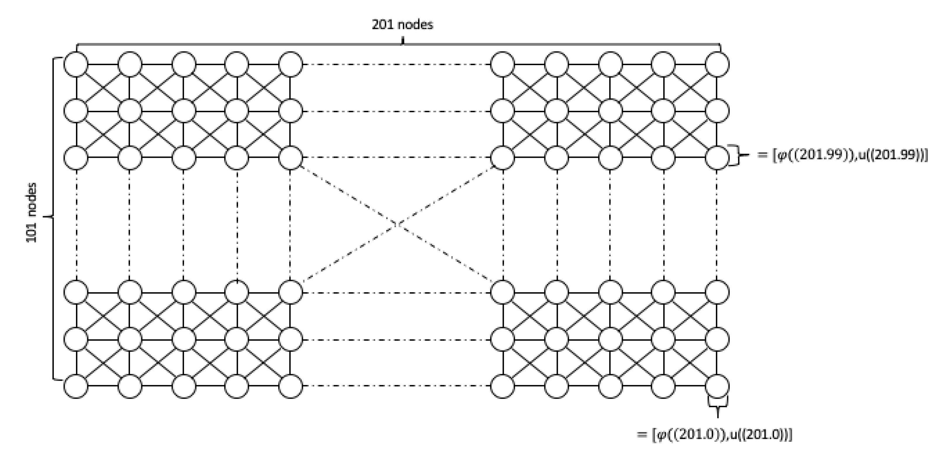
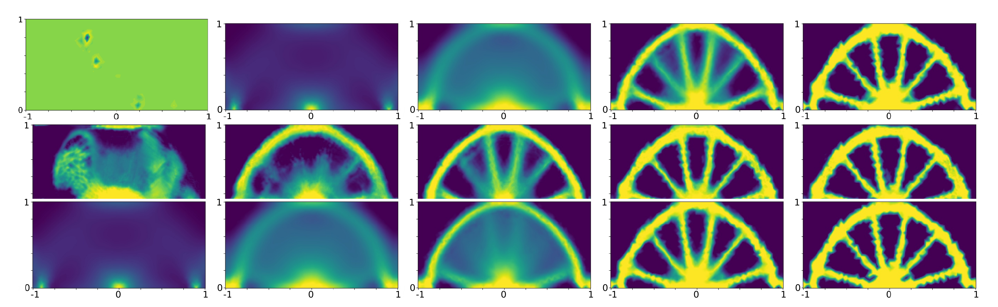
Table 1.
Comparison of metrics between Algorithms A1 and 1.
| Method | Applied Load g | Converges after | Evaluation of | Compliance |
|---|---|---|---|---|
| Algorithm A1 | 538 | 1475.39 | 1173.22 | |
| Algorithm 1 | 441 | 1206.49 | 1148.66 |
Table 2.
Comparison of metrics between Algorithms A2 and 2.
| Method | Converges after | Evaluation of | Compliance | Samples |
|---|---|---|---|---|
| Algorithm A2 | 490 | 765.85 | 729.20 | 224 |
| Algorithm 2 | 517 | 744.11 | 708.61 | 224 |
| Algorithm 2 | 500 | 760.26 | 723.24 | 224 |
Table 3.
Comparison of metrics between Algorithms A1 and 1.
| Method | Applied Load g | Converges after | Evaluation of | Compliance |
|---|---|---|---|---|
| Algorithm A1 | 538 | 1475.39 | 1173.22 | |
| Algorithm 1 | 441 | 1206.49 | 1148.66 | |
| Algorithm A1 (see Figure 8a) | 473 | 1487.39 | 1416.46 | |
| Algorithm 1 (see Figure 8a) | 517 | 1475.05 | 1405.39 | |
| Algorithm A1 (see Figure 8b) | 457 | 1115.66 | 1062.41 | |
| Algorithm 1 (see Figure 8b) | 497 | 1049.91 | 1042.58 | |
| Algorithm A1 (see Figure 8c) | 470 | 1042.18 | 992.28 | |
| Algorithm 1 (see Figure 8c) | 447 | 1048.44 | 998.34 |
Table 4.
Comparison of metrics between Algorithms A1, 1 and 3.
| Method | Applied Load g | Computation Time | Converges after | Evaluation of | Compliance |
|---|---|---|---|---|---|
| Algorithm A1 | 4 min 43 s | 538 | 1475.39 | 1173.22 | |
| Algorithm 1 | 4 min 05 s | 441 | 1206.49 | 1148.66 | |
| Algorithm 3 | 4 min 34 s | 425 | 1209.24 | 1151.27 | |
| Algorithm A1 | 4 min 31 s | 473 | 1487.39 | 1416.46 | |
| Algorithm 1 | 4 min 14 s | 517 | 1475.05 | 1405.39 | |
| Algorithm 3 | 4min 34 s | 436 | 1209.24 | 1151.27 | |
| Algorithm A1 | 4 min 50 s | 457 | 1115.66 | 1062.41 | |
| Algorithm 1 | 4 min 21 s | 497 | 1049.91 | 1042.58 | |
| Algorithm 3 | 4 min 41 s | 484 | 1082.62 | 1031.62 | |
| Algorithm A1 | 5 min 11 s | 470 | 1042.18 | 992.28 | |
| Algorithm 1 | 4 min 42 s | 447 | 1048.44 | 998.34 | |
| Algorithm 3 | 4 min 43 s | 542 | 1041.28 | 992.16 | |
| Algorithm A1 | 2 min 17 s | 365 | 845.93 | 805.94 | |
| Algorithm 1 | 2 min 13 s | 346 | 852.36 | 811.15 | |
| Algorithm 3 | 2 min 59 s | 366 | 848.52 | 808.40 |
Publisher’s Note: MDPI stays neutral with regard to jurisdictional claims in published maps and institutional affiliations. |
© 2022 by the authors. Licensee MDPI, Basel, Switzerland. This article is an open access article distributed under the terms and conditions of the Creative Commons Attribution (CC BY) license (https://creativecommons.org/licenses/by/4.0/).
Share and Cite
MDPI and ACS Style
Eigel, M.; Haase, M.; Neumann, J. Topology Optimisation under Uncertainties with Neural Networks. Algorithms 2022, 15, 241. https://0-doi-org.brum.beds.ac.uk/10.3390/a15070241
AMA Style
Eigel M, Haase M, Neumann J. Topology Optimisation under Uncertainties with Neural Networks. Algorithms. 2022; 15(7):241. https://0-doi-org.brum.beds.ac.uk/10.3390/a15070241
Chicago/Turabian StyleEigel, Martin, Marvin Haase, and Johannes Neumann. 2022. "Topology Optimisation under Uncertainties with Neural Networks" Algorithms 15, no. 7: 241. https://0-doi-org.brum.beds.ac.uk/10.3390/a15070241
Note that from the first issue of 2016, this journal uses article numbers instead of page numbers. See further details here.