1. Introduction
Trust-region methods are a popular class of algorithms for finding the solutions of nonlinear minimization optimization problems [
1,
2]. Trust-region algorithms build a model of the objective function in a neighborhood of the incumbent solution. The region in which the model function behaves similarly to the objective function is called the
trust region and is defined through a
trust-region radius. The optimization algorithm then finds a point in the trust region at which the model sufficiently decreases. This step is known as the
trust-region sub-problem, and the point that provides a sufficient decrease is called the
trial point. The value of the objective function is then computed at the trial point. If the ratio of the
achieved reduction versus the
reduction in the model is sufficient, then the incumbent solution is updated and set to be equal to the trial point. If the ratio is not sufficient, then the
trust-region radius is decreased. This method iterates until a stopping condition implies that a local minimizer has been located.
Extensive research has been done on this topic since 1944, when Levenberg published what is known to be the first paper related to trust-region methods [
3]. Early work on trust-region methods includes the work of Dennis and Mei [
4], Dennis and Schnabel [
5], Fletcher [
6], Goldfeldt, Quandt, and Trotter [
7], Hebden [
8], Madsen [
9], Moré [
10,
11], Moré and Sorensen [
12], Osborne [
13], Powell [
14,
15,
16,
17,
18], Sorensen [
19,
20], Steihaug [
21], Toint [
22,
23,
24,
25], and Winfield [
26,
27], to name a few. The name
trust region seems to have been used for the first time in 1978 by Dennis in [
28].
In the works mentioned above, trust-region methods were designed and analyzed under the assumption that first-order information about the objective function is available and that second-order information (i.e., Hessians) may, or may not, be available. In the case in which both first-order and second-order information is not available, or it is hard to directly obtain,
derivative-free trust-region (DFTR) methods can be used. This type of method has become more popular in the last two decades due to the rise of blackbox optimization problems. Early works on DFTR methods include those of Conn, Scheinberg, and Toint [
29], Marazzi and Nocedal [
30], Powell [
31,
32], and Colson and Toint [
33], to name a few.
In 2009, the convergence properties of general DFTR algorithms for unconstrained optimization problems were rigorously investigated [
34]. The pseudo-code of an algorithm that converges to a first-order critical point and the pseudo-code of an algorithm that converges to a second-order critical point were provided. A complete review of the DFTR methods for unconstrained optimization problems is available in [
35] (Chapters 10 and 11) and [
36] (Chapter 11). There now exist several DFTR algorithms for solving unconstrained optimization problems, such as Advanced DFO-TRNS [
37], BOOSTERS [
38], CSV2 [
39], DFO [
29,
40], UOBYQA [
31], and WEDGE [
30]. In recent years, DFTR algorithms have also been developed for constrained optimization problems. When an optimization problem is bound-constrained, some of the algorithms available in the literature are BC-DFO [
41], BOBYQA [
42], ORBIT [
43,
44], SNOBFIT [
45], and TRB-POWELL [
46]. Other DFTR algorithms dealing with more general constrained optimization problems include CONDOR [
47], CONORBIT [
48], DEFT-FUNNEL [
49], LCOBYQA [
50], LINCOA [
51], and S [
52].
We define a
blackbox as any process that returns an output whenever an input is provided, but where the inner mechanism of the process is not analytically available to the optimizer [
36]. In this paper, we consider a situation in which the objective function,
is obtained by manipulating several blackboxes. For instance,
F could be the product of two functions, say,
and
, where the function values for
are obtained through one blackbox and the function values for
are obtained through a different blackbox. An objective function that is defined by manipulating more than one function is called a
composite objective function.
Composite objective functions have inspired a particular direction of research under the assumption that the functions involved do not have the same computational costs. For instance, Khan et al. [
53] developed an algorithm for minimizing
, where
is smooth with known derivatives,
h is a known nonsmooth piecewise linear function, and
f is smooth but expensive to evaluate. In [
54], Larson et al. investigated the minimization problem
, where
h is nonsmooth and inexpensive to compute and
f is smooth, but its Jacobian is not available. Recently, Larson and Menickelley developed algorithms for bound-constrained nonsmooth composite minimization problems in which the objective function
F has the form
, where
h is cheap to evaluate, and
f requires considerable time to evaluate.
These ideas have led to research on more general calculus-based approaches to approximating gradients or Hessians of composite functions. In [
55,
56,
57], the authors provided calculus rules (integer power, product, quotient, and chain) for
(generalized) simplex gradients. These results were advanced to the
(generalized) centered simplex gradient in [
58] and to the
(generalized) simplex Hessian in [
59]. In [
60], a unified framework that provides general error bounds for gradient and Hessian approximation techniques by using calculus rules was presented.
Previous research has shown that a calculus-based approach to approximating gradients or Hessians can be substantially more accurate than a non-calculus-based approach in several situations [
55,
58,
59,
60]. However, it is still unclear if these theoretical results translate to a significant improvement in a derivative-free algorithm. The main goal of this paper is to compare two versions of a DFTR algorithm designed to solve a box-constrained blackbox optimization problem in which the objective function is a composite function: one that employs a calculus-based approach and one that does not employ a calculus-based approach. It is worth emphasizing that it is not our intention to show that the DFTR algorithm developed in this paper is better than state-of-the-art derivative-free algorithms. The main goal is to analyze any benefits resulting from using a calculus-based approach in a DFTR algorithm designed to minimize a composite objective function.
This paper is organized as follows. In
Section 2, the context is established and fundamental notions related to the topic of this paper are presented. In
Section 3, the pseudo-code of the DFTR algorithm is introduced, and details related to the algorithm are discussed. In
Section 4, numerical experiments are conducted to compare the calculus-based approach with the non-calculus-based approach. In
Section 5, the results of the numerical experiments are scrutinized. Lastly, the main results of this paper, the limitations of this paper, and future research directions are briefly discussed in
Section 6.
2. Background
Unless otherwise stated, we use the standard notation found in [
36]. We work in the finite-dimensional space
with the inner product
. The norm of a vector is denoted as
and is taken to be the
norm. Given a matrix
the
induced matrix norm is used.
We denote by
the closed ball centered at
with radius
The identity matrix in
is denoted by
, and the vector of all ones in
is denoted by
The
Minkowski sum of two sets of vectors
A and
B is denoted by
That is,
In the next sections, we will refer to a calculus-based approach and a non-calculus approach to approximate gradients and Hessians. Let us clarify the meanings of these two approaches.
We begin with the non-calculus-based approach. Let and let be a quadratic interpolation of F at using distinct sample points poised for quadratic interpolation. An approximation of the gradient of F at , denoted by is obtained by computing and an approximation of the Hessian of F at , denoted by is obtained by computing
We now explain the calculus-based approach. Let
be constructed using
and
. Let
and
be quadratic interpolation functions of
and
, respectively. When a calculus-based approach is employed and the composite objective function
F has the form
then
and
Similarly, when the composite objective function
F has the form
then (assuming
)
and
To compute
the technique called the (generalized) simplex Hessian is utilized [
59]. When the two matrices involved in the computation of the simplex Hessian are square matrices that have been properly chosen, the simplex Hessian is equal to the Hessian of the quadratic interpolation function. The formula for computing simplex Hessians is based on simple matrix algebra. Hence, this technique is straightforward to implement in an algorithm. The formula for computing the simplex Hessian requires the computation of
simplex gradients.
Definition 1 ([
55]). (Simplex gradient).
Let . Let be the point of interest. Let with The simplex gradient
of f at over T is denoted by and defined bywhere Definition 2 ([
59]). (Simplex Hessian).
Let and let be the point of interest. Let and with The simplex Hessian
of f at over S and T is denoted by and defined bywhere The simplex gradient and simplex Hessian do not necessarily require the matrices
S and
T to be square matrices with a full rank. These two definitions may be generalized by using the Moore–Penrose pseudoinverse of a matrix [
55,
59].
Last, we recall the definition of a fully linear class of models.
Definition 3 ([
36]). (Class of fully linear models).
Given and we say that is a class of fully linear models of f at x parametrized by Δ
if there exists a pair of scalars and such that, given any the model satisfies
Note that a fully linear model is equivalent to a model that is
order-1 gradient accurate and
order-2 function accurate based on the definitions introduced in [
56].
We are now ready to introduce the pseudo-code of the DFTR algorithm that will be used to compare the calculus-based approach with the non-calculus-based approach.
3. Materials and Methods
In this section, the algorithm designed to minimize a box-constrained blackbox optimization problem involving a composite objective function is described. The algorithm will be used to perform our comparison between the calculus-based approach and the non-calculus-based approach in
Section 4.
Let
be the maximum trust-region radius allowed in the DFTR algorithm. The minimization problem considered is
where
is twice continuously differentiable on
where
, and the inequalities
are taken component-wise. It is assumed that
F is a composite function obtained from two blackboxes with similar computational costs.
Before introducing the pseudo-code of the algorithm, let us clarify some details about the model function and the trust-region sub-problem.
The model function built at an iteration
k will be denoted by
The model is a quadratic function that can be written as
where
denotes an approximation of the gradient
is a symmetric approximation of the Hessian
, and
is the independent variable.
When a calculus-based approach is used, both
and
are built by using the calculus-based approach presented earlier in
Section 2. Similarly, if the non-calculus-based approach is used, then both
and
are built with the non-calculus approach. We define the sampling radius,
, as the maximum distance between the incumbent solution
and a sampling point used to build the approximations
and
The trust-region subproblem solved in the DFTR algorithm (Step 2 of Algorithm 1) at an iteration
k is
where
is the trust-region radius at an iteration
Recall that the first-order necessary condition for solving (
5) is that the
projected gradient is equal to zero. The projected gradient of the model function
at
onto the feasible box, which is delimited by
ℓ and
u where
, is defined by
where the projection operator,
is defined component-wise by
Similarly, we define the projected gradient of the objective function at
onto the box by
Next, the pseudo-code of our DFTR algorithm is presented. This is essentially the pseudo-code in [
34] (Algorithm 4.1), but adapted for a box-constrained problem (see also Algorithm 10.1 in [
35] and Algorithm 2.1 in [
61]). The algorithm is a first-order method in the sense that it converges to a first-order critical point.
Several details about the pseudo-code require some clarification. The procedure employed in our algorithm to build the model function at an arbitrary iteration
k guarantees that the model
is fully linear on
To see this, first note that when a model
is built in Algorithm 1, we always have that the sampling radius
It is known that the gradient of a quadratic interpolation function built with
sample points poised for quadratic interpolation is
The Hessian of this quadratic interpolation is
It was shown in [
60] that the calculus-based approach to approximating gradients described in (
1) and (
3) is
It was also shown in [
59,
60] that the calculus-based approach to approximating the Hessians described in (
2) and (
4) was
Hence,
and
are
-accurate. The next proposition shows that if
and
are both
-accurate approximations of the gradient and Hessian at
, respectively, then the model function
is fully linear on
Proposition 1. Let and Assume that , where k is any iteration of Algorithm 1. Let the model function be defined as in Equation (7). If is an -accurate approximation of the gradient of F at and is an -accurate approximation of the Hessian of F at then the model is fully linear on Proof. For any
we have
where
is the Lipschitz constant of
on
and
Note that
is bounded above, since
Since
F is twice continuously differentiable on the box constraint, we have
for some nonnegative scalar
M independently of
Therefore,
Letting
we obtain
Hence, the first property in Definition 3 is verified. The second property can be obtained by using a similar process to that used in [
62] (Proposition 19.1). Therefore, the model
is fully linear on
□
| Algorithm 1 DFTR pseudo-code. |
Step 0: Initialization. Choose a feasible initial point an initial trust-region radius an initial sampling radius and a maximal trust-region radius Build an initial fully linear model on . Denote by and the gradient and Hessian of the initial model at Choose the constants (with , Set for Step 1: Criticality step. If and , stop. Return If and , set If , set update the model to make it fully linear on Step 2: Trust-region sub-problem. Find an approximate solution to the trust-region sub-problem ( 8). Step 3: Acceptance of the trial point. If , set and build a fully linear model Otherwise (), set and Step 4: Trust-region radius update. If , set If , attempt to improve the accuracy of the model. Increment k by one and go to Step 1. end for
|
It follows from Proposition 1 that Algorithm 1 always builds a fully linear model on
In [
61], Hough and Roberts analyzed the convergence properties of a DFTR algorithm for an optimization problem of the form
where
is closed and convex with a nonempty interior and
The main algorithm developed in their paper, Algorithm 2.1, follows the same steps as those of our algorithm. Since a box constraint is a convex closed set with a nonempty interior, the convergence results that were proven in [
61] may be applied to Algorithm 1. For completeness, we recall the three assumptions and convergence results of [
61].
Assumption 1. The objective function F is bounded below and continuously differentiable. Furthermore, the gradient is Lipschitz continuous with the constant in
Assumption 2. There exists such that for all k.
Assumption 3. There exists a constant such that the computed step satisfies , and the generalized Cauchy decrease condition is Theorem 1. Suppose that Algorithm 1 is applied to the minimization problem (5). Suppose that Assumptions 1–3 hold. Then, To conclude this section, we provide details on the different choices made while implementing Algorithm 1.
3.1. Implementing the Algorithm
Let us begin by specifying the value used for all of the parameters involved in the algorithm. Our choices were influenced by some preliminary numerical results and the values proposed in the literature, such as [
1] (Chapter 6).
In our implementation, the parameters are set to:
To build an approximation of the Hessian
we compute a simplex Hessian, as defined in Definition 2. Two matrices of directions
S and
T must be chosen; at every iteration
k, the matrices
and
are set to
Multiplying the identity matrix by
to form
and
guarantees that the sampling radius for building an approximation of the Hessian is equal to
Setting
and
in this fashion creates
distinct sample points poised for quadratic interpolation. This implies that the simplex Hessian is equal to the Hessian of the quadratic interpolation function [
59]. Clearly, other matrices
and
could be used, and
does not necessarily need to be equal to
, nor to always be a multiple of the identity matrix for every iteration
More details on how to choose
S and
T so that the resulting set of sample points is poised for quadratic interpolation can be found in [
59].
To build an approximation of the gradient the gradient of the quadratic interpolation function built using the same sample points used to obtain is simply computed. Therefore, building a model requires function evaluations.
Note that the sample points utilized to build and may be outside of the box constraint. This is allowed in our implementation.
To solve the trust-region sub-problem, the Matlab command quadprog with the algorithm trust-region-reflective is used. In theory, this method satisfies Assumption 3.
Based on the preliminary numerical results, the version of Algorithm 1 that is utilized to conduct the numerical experiments in this section does not attempt to improve the accuracy of the model in Step 4. The results obtained suggest that rebuilding a new model function when decreases the efficiency of our algorithm.
Reducing Numerical Errors
We next discuss two strategies that decrease the risk of numerical errors. When the sampling radius
is sufficiently small, numerical errors occur while computing
and
, and this can cause
and
to be very bad approximations of the gradient and Hessian at
To avoid this situation, a minimal sampling radius
is defined. Every time the sampling radius
is updated in Algorithm 1 (this may happen in Step 1 or Step 5), the rule implemented is the following:
In our implementation, Numerical errors can occur with relatively large values of the sampling radius The following example illustrates this situation. This motivates our choice of setting
Example 1. Let Set where Note that the sampling radius is Table 1 presents the relative error of the simplex Hessian which is denoted by We see that numerical errors occur at a value of between and .
A maximal sampling radius
is also defined to ensure that the sampling radius
does not become excessively large when the trust-region radius is large. The parameter is set to
Therefore, after checking (
10), the following update on
is performed:
In Step 3, in the computation of
the denominator satisfies
As mentioned in [
1] (Section 17.4), to reduce the numerical errors, we use (
11) to compute this value.
To compute the ratio
we again follow the advice given in [
1] (Section 17.4.2) and proceed in the following way. Let
, where
is the relative machine precision. Let
Define
3.2. Data Profiles
To perform the comparisons in the next section, data profiles were built [
63]. The convergence test for the data profiles is
where
is a tolerance parameter and
is the best known minimum value for each problem
p in
Let
be the number of function evaluations required to satisfy (
12) for a problem
by using a solver
given a maximum number of function evaluations
In this paper, the parameter is
, where
is the dimension of the problem
Note that
is set to
∞ if (
12) is not satisfied after
function evaluations. The data profile of a solver
is defined by
Three different values of will be used to build the data profiles: .
3.3. Experimental Setup
Algorithm 1 was implemented in Matlab 2021a while using both the calculus-based and non-calculus-based approach to approximating gradients and Hessians. The computer that was utilized had an Intel Core i7-9700 CPU at 3.00 GHz and 16.0 GB of DDR4 RAM at 2666 MHz on a 64-bit version of Microsoft Windows 11 Home. These implementations were tested on a suite of test problems, which are detailed below. The Matlab function fmincon was also tested on each problem for all of the experiments mentioned below. This was done as a validation step to demonstrate that Algorithm 1 was correctly implemented (and reasonably competitive with respect to the currently used methods).
To conclude this section, we present the details of the different situations tested for the product rule and the quotient rule.
3.3.1. Numerical Experiment with the Product Rule
In these numerical experiments, the composite objective function F had the form where Three different situations were considered:
and were linear functions;
was a linear function and was a quadratic function;
and were quadratic functions.
Recall that a linear function
has the form
where b
and
A quadratic function
has the form
where
is a symmetric matrix. At the beginning of each experiment, the seed of the random number generator was fixed to 54321 by using the command rng. The dimension of the space was between 1 and 30, and it was generated with the command randi. All integers were generated with
randi. In each experiment, the coefficients involved in
and
were integers between −10 and 10 inclusively. Each component of the starting point
was an integer between −5 and 5 inclusively. The box constraint was built in the following way:
This created a randomly generated test problem of the form of (
5). This problem was solved via Algorithm 1 by using the starting point
and by using both versions—the calculus-based approach and the non-calculus-based approach. Each of the three situations listed above was repeated 100 times. Each time, all of the parameters were generated again: the dimension
n, the starting point
the box constraint
, and the functions
3.3.2. Numerical Experiment with the Quotient Rule: Easy Case
In these experiments, the composite objective function took the form
where
was either a linear function or a quadratic function for
. We began by building the function
such that its real roots, if any, were relatively far from the box constraint. To do so, each component of the starting point
was taken to be an integer between 1 and 100 inclusively. The coefficients in
are taken to be integers between 1 and 10 inclusively. When
was a quadratic function, note that having all positive entries in the matrix
A did not necessary imply that
A was positive semi-definite. The box constraint was built in the same fashion as in the previous experiment. Thus, the bounds were
Note that if is a root of then r must have at least one negative component. Since and is an increasing function, there is no root of in the box constraint. Hence, F is twice continuously differentiable on the box constraint. The following four situations were tested:
and were linear functions;
was a linear function and was a quadratic function;
was a quadratic function and was a linear function;
and were quadratic functions.
Each situation was repeated 100 times.
3.3.3. Numerical Experiment with the Quotient Rule: Hard Case
Last, the quotient rule was tested again, but this time, the function was built so that there was a root of near (but not within) the box constraint. The differences from the previous quotient experiments were the following. Each component of the starting point was taken as an integer between −5 and 5 inclusively. Let , where The coefficients in were taken to be between −10 and 10 inclusively. Before generating the constant c in the minimum value on the box constraint of , say, was found. Then, c was set to Hence, was built such that the minimum value of on the box constraint was 0.001 and for all x in the box constraint.
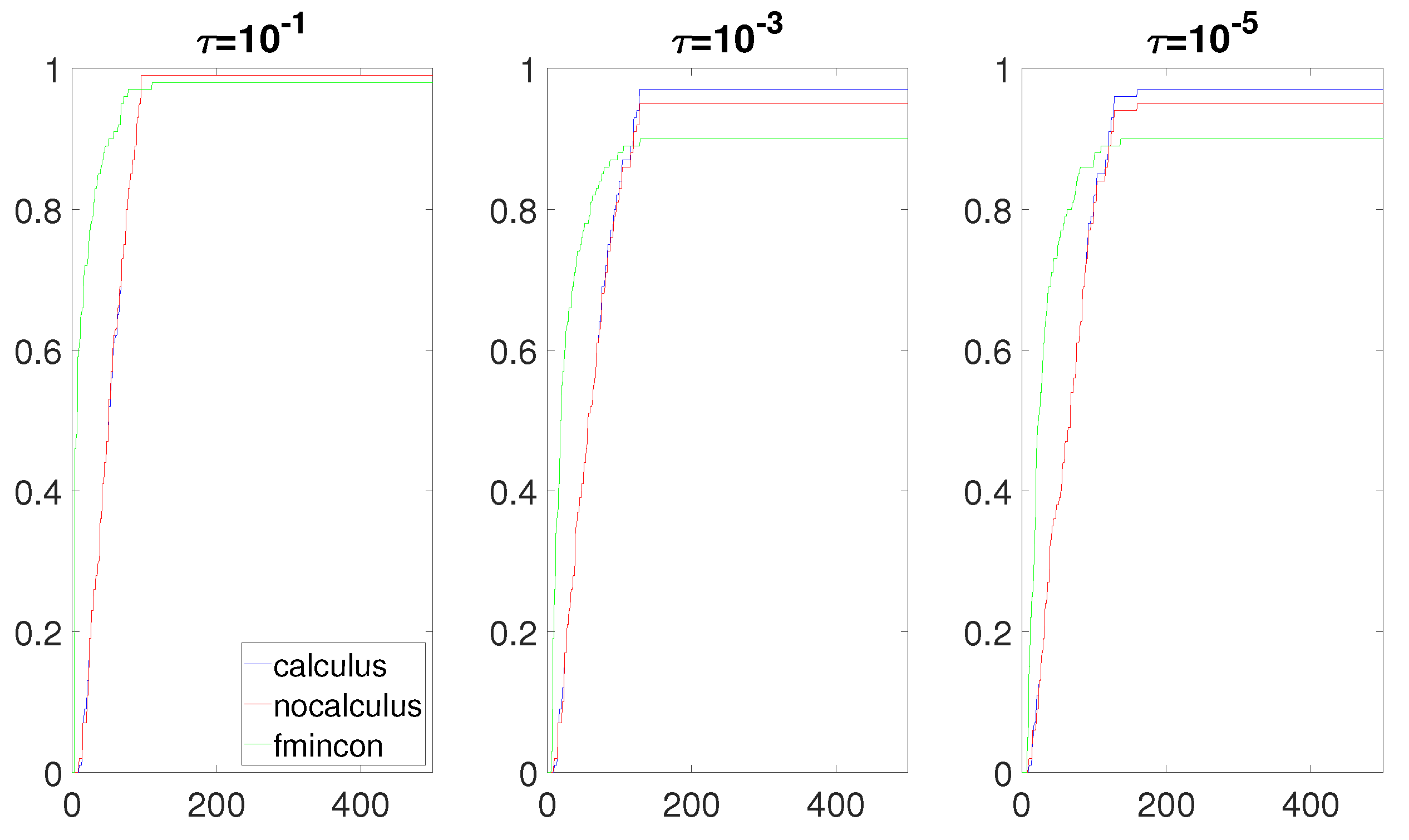
4. Results
In this section, the data profiles for each of the three experiments are presented. We begin by presenting the data profiles for the product rule. The following nine data profiles (three data profiles per situation) were obtained (
Figure 1,
Figure 2 and
Figure 3). In the following figures, the
x-axis represents the independent variable
, as defined in
Section 3.2. The
y-axis represents the percentage of problems solved. For a given tolerance parameter
, the robustness of an algorithm was obtained by looking at the value of its curve at the greatest value of
in the figures. For example, fmincon solved 100% of the problems for all three values of
in
Figure 1. For a given percentage of problems solved, the curve with the smallest value of
represented the most efficient algorithm, as it used fewer function evaluations to solve a certain percentage of the problems. For example, when
in
Figure 1, the fmincon algorithm was the most efficient and the most robust of all three algorithms. Roughly speaking, if a curve is on top of all other curves in a data profile, then it was the most efficient and the most robust algorithm on this set of problems for a given value of
Testing different values of
provides information about the level of accuracy that an algorithm can achieve. Small values of
provide information about the capabilities of an algorithm for finding accurate minimizers, and large values of
provide information about the capabilities of an algorithm for finding rough approximations of the minimizers.
6. Conclusions
When dealing with a composite objective function, the numerical results obtained in
Section 4 clearly suggest that a calculus-based approach should be used. In particular, in all cases tested, the calculus-based approach was better or as good as the non-calculus-based approach. Since a calculus-based approach is not more difficult to implement than a non-calculus-based approach, the former approach seems to be the best approach to implement and use whenever a composite objective function is optimized.
When the composite objective function was a quotient (
) and there was a real root of
near the box constraint, the calculus-based approach greatly outperformed the other methods. In this case, the sampling radius needed to be very small to obtain a relatively accurate gradient and Hessian when using the non-calculus-based approach. In some situations, numerical errors may occur before obtaining the accuracy required for convergence. In general, based on the results obtained, it seems reasonable to think that a calculus-based approach will outperform a non-calculus-based approach when the Lipschitz constant of the gradient and∖or Hessian of
F on the box constraint are large numbers. By increasing the range of numbers allowed to generate the functions
and
when using the product rule in the experiment described in
Section 3.3.1, it is relatively easy to create a test set of problems in which the differences in performance between the calculus-based approach and the non-calculus-based approach are more pronounced than the results presented in this paper (
Figure 1,
Figure 2 and
Figure 3), which are in favor of the calculus-based approach. However, the gain in performance is not as drastic as the results obtained with the quotient rule in our third experiment (
Figure 8,
Figure 9,
Figure 10 and
Figure 11). Further investigation is needed to determine situations in which the calculus-based approach significantly outperforms the non-calculus-based approach when using the product rule.
We remark that our implementation of Algorithm 1 is simple. This is intentional, as the goal is to compare the calculus-based approach with the non-calculus-based approach. Nonetheless, we remark that, recently, Nocedal et al. found that a DFTR algorithm that used quadratic models built from a forward-finite-difference gradient and a forward-finite-difference Hessian can be surprisingly competitive with state-of-the-art derivative-free algorithms [
64]. From our perspective, now that the calculus-based approach has been established as the superior method within a model-based derivative-free algorithm, the next logical step is to use this knowledge to improve current state-of-the-art software (e.g., [
65]). Applying a calculus-based approach to real-world optimization problems is, then, the obvious direction of future research.
Another direction to explore is inspired by model-based methods for high-dimensional blackbox optimization [
66]. In [
66], the authors used subspace decomposition to reduce a high-dimensional blackbox optimization problem into a sequence of low-dimensional blackbox optimization problems. At each iteration, the subspace was rotated, requiring new models to be frequently constructed. An examination of whether calculus rules could be adapted to help in this situation would be an interesting direction for future research.
This further links to a direction of future research based on underdetermined gradient/Hessian approximations. An underdetermined approximation does not contain accurate information about all entries of a gradient/Hessian, but uses fewer function evaluations than the determined case. It would be valuable to explore if calculus-based approaches could be merged with underdetermined approximations to create more accuracy with a minimal increase in function evaluations.


