
Acoustic Echo Cancellation with the Normalized Sign-Error Least Mean Squares Algorithm and Deep Residual Echo Suppression


Andrew and Erna Viterbi Faculty of Electrical & Computer Engineering, Technion–Israel Institute of Technology, Technion City, Haifa 3200003, Israel
*
Authors to whom correspondence should be addressed.
Algorithms 2023, 16(3), 137; https://0-doi-org.brum.beds.ac.uk/10.3390/a16030137
Submission received: 30 December 2022
/
Revised: 1 February 2023
/
Accepted: 7 February 2023
/
Published: 3 March 2023
(This article belongs to the Special Issue Deep Learning Architecture and Applications)
Abstract
:This paper presents an echo suppression system that combines a linear acoustic echo canceller (AEC) with a deep complex convolutional recurrent network (DCCRN) for residual echo suppression. The filter taps of the AEC are adjusted in subbands by using the normalized sign-error least mean squares (NSLMS) algorithm. The NSLMS is compared with the commonly-used normalized least mean squares (NLMS), and the combination of each with the proposed deep residual echo suppression model is studied. The utilization of a pre-trained deep-learning speech denoising model as an alternative to a residual echo suppressor (RES) is also studied. The results showed that the performance of the NSLMS is superior to that of the NLMS in all settings. With the NSLMS output, the proposed RES achieved better performance than the larger pre-trained speech denoiser model. More notably, the denoiser performed considerably better on the NSLMS output than on the NLMS output, and the performance gap was greater than the respective gap when employing the RES, indicating that the residual echo in the NSLMS output was more akin to noise than speech. Therefore, when little data is available to train an RES, a pre-trained speech denoiser is a viable alternative when employing the NSLMS for the preceding linear AEC.
1. Introduction
Acoustic echo cancellation is a long-standing problem in real-life telecommunication scenarios where a near-end speaker communicates with a far-end speaker. A loudspeaker plays the far-end signal, and a microphone captures the echo of the loudspeaker signal, and the near-end signal and background noise [1].
Traditional acoustic echo cancellers (AECs) employ linear adaptive filters [2]. Linear AECs commonly use the least mean squares (LMS) algorithm [3,4] and its normalized version, the normalized LMS (NLMS) [5,6]. The improvement introduced by the normalization is that the step size can be set independently of the reference signal’s power [7]. Variants of the LMS and NLMS algorithms are the sign-error LMS (SLMS), and normalized SLMS (NSLMS) algorithms [8]. In contrast to the NLMS, the NSLMS adjusts the weight for each filter tap, based on the polarity (sign) of the error signal. Several studies have shown the advantages of the NSLMS over the NLMS. For example, Freire and Douglas [9] used the NSLMS adaptive filter to cancel geomagnetic background noise in magnetic anomaly detection systems and demonstrated its superiority over the NLMS. Pathak et al. [10] utilized the NSLMS adaptive filter to perform speech enhancement in noisy magnetic resonance imaging (MRI) environments. According to their experiments, the NSLMS achieved faster convergence than the NLMS, and residual noise produced by the NSLMS had characteristics of white noise. In contrast, residual noise produced by the NLMS was more structured.
The linear AECs lack the ability to cancel the nonlinear components of the echo. Therefore, further suppression of the residual echo is required, and a residual echo suppressor (RES) is typically employed. While traditional residual echo suppression relies on filter-based techniques [11,12], recent advances in deep learning have shifted the focus toward neural network-based approaches [13,14,15,16]. Under challenging real-life conditions, for example, low signal-to-echo ratios (SERs) and changing acoustic echo paths, the performance of the linear AEC preceding the RES model has a significant impact on the overall performance. Hence, it may be beneficial to investigate the AECs in conjunction with deep-learning models for residual echo suppression.
The output of a linear AEC is expected to contain a distorted weaker version of the echo signal, while keeping the near-end signal almost distortionless. Therefore, denoising the estimated near-end signal with a designated speech denoiser might suppress the residual echo, while eliminating other noises. Research on deep-learning-based speech enhancement algorithms has seen significant progress over the last few years, with many models exhibiting excellent performances [17,18,19]. For a speech denoiser to achieve good performance as an RES, the AEC must produce residual echo that closely resembles noise, rather than human speech.
In this paper, two aspects of residual echo suppression were investigated: the impact of the preceding linear AEC on the performance of the residual echo suppression deep-learning model and the utilization of a pre-trained speech denoiser as an alternative to an RES. In addition, an echo suppression system, that employs NSLMS to perform linear acoustic echo cancellation and a deep complex convolutional recurrent network (DCCRN) [18] to achieve residual echo suppression, is proposed. The performances of the NSLMS and the commonly-used NLMS algorithms were compared, and the utilization of a speech denoiser to the output of the linear AEC to suppress the residual echo and additional noises was evaluated. The results showed that the performances of systems using NSLMS were superior to those using NLMS in all settings. This suggested that NSLMS was better suited for acoustic echo cancellation and residual echo suppression tasks, emphasizing the importance of choosing the right linear AEC. Additionally, the performance of the pre-trained denoiser in combination with each linear AECs was investigated to determine which of the outputs contained residual echo that resembled noise more closely than speech. The results indicated that, contrary to the NLMS, the outputs of the NSLMS were more akin to noise than speech. Therefore, the preceding linear AEC choice had an even more significant impact when employing a pre-trained speech denoiser model for the residual echo suppression task. With the NSLMS, a speech denoiser might be a suitable alternative when insufficient data is available to train an RES model. Finally, the advantages and efficacy of the proposed RES model over a larger pre-trained denoiser model are shown. To summarize the contributions of the presented study, the main findings are highlighted below:
- The performance of the NSLMS is superior to that of the common NLMS, both as a standalone linear AEC and combined with a deep-learning residual echo suppressor. More generally, the reported findings indicated that the linear AEC significantly impacted the performance of the following residual echo suppressor and should be carefully chosen.
- When combined with a pre-trained speech denoiser, the NSLMS brings a more significant performance improvement than when combined with a residual echo suppressor. This indicated that the outputs of the NSLMS were less structured and more akin to noise than the NLMS outputs. Therefore, with the NSLMS, employing a pre-trained speech denoiser might be a viable alternative to training a residual echo suppressor.
- The DCCRN architecture, initially proposed for speech enhancement, is offered to perform residual echo suppression. While requiring only a minor modification to adapt to the residual echo suppression task, the proposed residual echo suppressor outperformed the larger, pre-trained speech denoiser.
The presented study focused on challenging real-life scenarios, such as echo–path changes, low signal-to-echo ratios (SERs), and real-time considerations.
Following is the outline of the manuscript. In Section 2, formulation of the residual echo suppression problem is provided, the relevant signals are denoted, the different systems and their components are described, and details regarding the datasets and experimental procedures are provided. In Section 3, the experimental results are provided. The results are discussed and interpreted in this section as well. The manuscript is concluded in Section 4.
2. Materials and Methods
This section is organized as follows. First, the different signals of concern are denoted and explained. A high-level overview of the residual echo suppression setting is also provided. Next, the different systems and system components are described in detail. Lastly, the training and evaluation data are described, and experimental, and implementation details are provided.
2.1. Problem Formulation
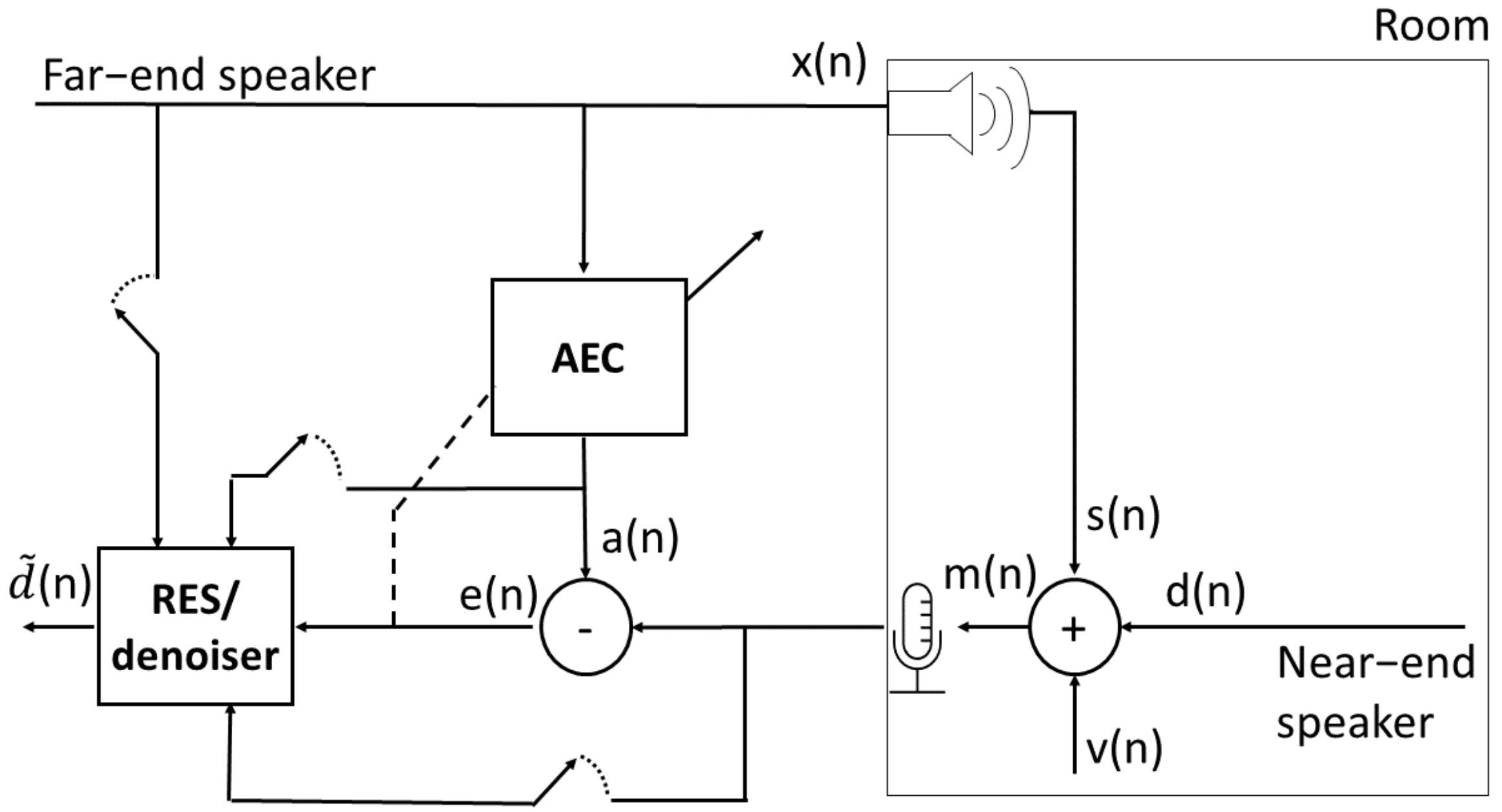
First, the different signals presented in the manuscript are denoted. The far-end reference signal is denoted by . The echoic loudspeaker signal is denoted by , and the near-end signal is denoted by . The value denotes the background noise. The microphone signal is given by:
The linear AEC receives as inputs, and , and outputs two signals: , the estimate of the echo signal , and the estimate of the noisy near-end signal, i.e., the error signal . The filter tap weights vector of length N is denoted by , where represents the transposed vector. Similarly, the far-end signal’s vector at time n and length N is denoted by .
The error signal contains noise and residual echo components. The goal was to enhance by further suppressing the residual echo and possibly removing noise. This is done either by a speech denoising model, in which case it receives as a single input to be denoised, or by an RES model, in which case it also receives as inputs , , and . The RES/denoiser block predicts . The problem’s setup and the related signals are depicted in Figure 1. When referring to the short-time Fourier transform (STFT) [20] domain transformations of the above signals, f denotes the frequency index, and k denotes the time index of the transformed signals. For example, is the STFT of .
2.2. System Components
A residual echo suppression system comprises a linear AEC and an RES model. Two linear AECs were compared: NSLMS and NLMS. For residual echo suppression, two alternatives were considered: the proposed RES model and a pre-trained speech-denoising model.
2.2.1. Linear Acoustic Echo Cancellers
For linear acoustic echo cancellation, an AEC with the NSLMS algorithm was employed. The algorithm operates in the subband domain by transforming the signals with uniform single-sideband filter banks [21]. The filters’ tap weights update equation for each subband is given by:
where is the step size, and is the signum function. The performance of NSLMS was compared to that of NLMS, for which the tap weights update equation is given by:
2.2.2. Residual Echo Suppression Model
The DCCRN [18] architecture, which employs a complex convolutional encoder–decoder structure and a complex long short-term memory (LSTM), was adopted for residual echo suppression. The model was initially developed for speech enhancement in the time–frequency (T–F) domain. It estimates a complex ratio mask (CRM) applied to the STFT of the input signal. For residual echo suppression, the model was adapted to have 4 input channels instead of one, and its inputs were all available signals: , , , and . The estimated CRM was applied to the STFT of the error signal, . Figure 2 depicts the model’s architecture.
The encoder and decoder branches of the model were symmetrical, where the outputs of each encoder block were used as the inputs of the next encoder block and as additional inputs to the decoder block of the same level. These connections between the different encoder and decoder blocks are termed skip connections. Skip connections have two advantages: they provide an alternative path for the gradient during back-propagation, which is beneficial for model convergence, and they allow re-use of features from the encoder in the decoder. Each encoder/decoder block comprised a complex 2-D convolution layer, a complex batch-normalization layer, and a real parametric rectified linear unit (PReLU) activation function [22], as depicted in Figure 3.
A complex 2-D convolution layer comprised two real 2-D convolution layers, each operating on the real and imaginary parts of its input. The output of a complex 2-D convolution layer, denoted by , is formulated as:
where and are the real and imaginary parts of the input, respectively, and are the real and imaginary convolution kernels, respectively, and ∗ is the convolution operation. Like the complex 2-D convolution layer, the complex LSTM layer comprised two real LSTM layers, denoted by and . The output of the complex LSTM, denoted by , is formulated as:
Further details regarding the original model’s architecture and the structure of the different layers can be found in [18].
Since a clean near-end signal is unavailable when training with real, recorded data, the noisy near-end signal was the training target. The training objective was the waveform loss, combined with the multi-resolution STFT magnitude loss adopted from [17]. For an estimated signal and its ground-truth , the loss is defined as:
where T denotes the total time steps number, is the norm, M is the number of STFT resolutions, and i is the resolution index.
2.2.3. Speech Denoising Model
As an alternative to the RES model, an off-the-shelf, pre-trained speech-denoising deep-learning model [17], which accepts a single input and outputs , was utilized. A speech-denoising model might be considered an alternative to an RES in cases where the residual echo resembles noise more closely than speech. In these cases, the residual echo might be suppressed while preserving the near-end speech. The utilized speech-denoising model was based on the DEMUCS architecture [23]. The model operated in the time domain, and similarly to DCCRN, it employed a convolutional encoder–decoder structure and an LSTM between the encoder and the decoder. A single encoder block consisted of two 1-D convolution layers. The activation function of the first convolution layer was the rectified linear unit (ReLU) [24] and the activation function of the second convolution layer was the gated linear unit (GLU) [25]. The output of the encoder block was passed to the next encoder block (or to the LSTM when it was the final encoder block) and to its matching decoder block via a skip connection. A decoder block received both the output of the matching encoder block and the output of the previous decoder block (or the output of the LSTM when it was the first decoder block). The inputs were summed element-wise. The structure of the decoder block mirrored that of the encoder block, except after the first convolution layer, a 1-D transpose convolution layer was employed to upsample the signal. The structure of the encoder and decoder blocks is depicted in Figure 4. The general structure of the speech-denoising model is depicted in Figure 5. Further details regarding the model’s architecture can be found in [17].
As mentioned in Section 1, the speech enhancement field is well-studied, with an abundance of excellent works and a variety of readily-available, pre-trained models trained on large and diverse datasets. With careful fine-tuning, the features learned by such pre-trained models might be effectively utilized for the residual echo suppression task. This might be especially effective when there is only a small amount of data to train a residual echo suppression model. Therefore, a pre-trained model, provided by the authors [17], was employed. The model was pre-trained on the Valentini dataset [26] and the INTERSPEECH 2020 deep noise suppression (DNS) challenge dataset [27]. The model was subsequently fine-tuned with the same training data used for training the RES models, once with the NSLMS outputs and once with the NLMS outputs. The loss function that was minimized is given in (6).
2.3. Datasets
Two datasets were employed for training the different models: the ICASSP 2021 AEC challenge synthetic dataset [28] and an independently recorded dataset. Unlike the synthetic data, the independent recordings were taken in real-life conditions with low SERs. Various scenarios were considered, including echo–path changes, variations in near-end source positions and distances from the microphone, and varying room sizes. A total of 11 h of speech data were taken from the LibriSpeech [29] corpus and the TIMIT [30] corpus. Spider MT503TM or Quattro MT301TM speakerphones (Shure Inc., Niles, IL, USA) were utilized to simulate low-SER scenarios. The loudspeaker and microphone were positioned 5 cm from each other in these devices. Echo path changes were simulated by moving a Logitech type Z120TM loudspeaker (Logitech International S.A., Lausanne, Switzerland), playing the echo signal. The loudspeaker’s distance from the microphone was either 1, , or 2 m. The near-end speech was simulated using mouth simulator type 4227-ATM of Bruel&Kjaer (Bruel&Kjaer, Naerum, Denmark). The distance of the mouth simulator from the microphone also varied between recordings and was either 1, , or 2 m from the microphone. Double-talk utterances always contained two different speakers, so the average overlap between the two was . Rooms of different sizes were used for the recordings (sizes varied between m3 and m3). Reverberation time () varied between and s. The training data SER was distributed on decibels, and the test data SER was distributed on decibels. Test data speakers were unique and not used in the training set. Further details regarding the data creation can be found in [14].
The ICASSP 2021 AEC challenge synthetic dataset was used to augment the training data. About h of data were generated, with different scenarios, including double-talk, far-end or near-end single-talk, with/without near-end noise, and likewise for far-end. In addition, several nonlinear distortions were applied, with different SERs and signal-to-noise ratios. Further details regarding the dataset can be found in [28].
2.4. Implementation Details
All signals were sampled with a sampling rate of 16 kHz. Initially, the input signals were transformed to the subband domain by uniform 32-band single-sideband filter banks [21]. Each subband consisted of 150 taps. These were the equivalent of filters in the time domain with 2400 taps and of length 150 ms.
For the RES model, the transformation of the input signals to the T-F domain was achieved by a 512-point STFT, resulting in 257 frequency bins. The STFT window length was 25 ms, and the hop length was ms. The number of convolution kernels for the different encoder layers was . The LSTM had two layers with a 128 hidden size. The model comprised M parameters. The Adam optimizer [31] was employed for model optimization. Training started with a learning rate of . The learning rate was decreased by a factor of 2 if the validation loss did not improve after 3 consecutive epochs. The mini-batch size was 16, and the training continued for a maximum number of 100 epochs.
The number of encoder and decoder blocks for the speech-denoising model was 5. The number of the first encoder block’s output channels was 64, and each encoder block doubled the number of channels. Subsequently, each decoder block halved the number of channels, where the output of the last decoder block consisted of 1 channel. The convolution kernel size was 8, and its stride was 4. The LSTM consisted of two layers, and its hidden size matched the number of channels of the last encoder block (and the number of channels of the first decoder block). The input to the model was normalized by its standard deviation. The model was pre-trained using the Valentini dataset [26] and the INTERSPEECH 2020 DNS challenge dataset [27]. The model comprised M parameters. For a fair comparison with the RES model, the causal version of the denoiser was employed. For both linear AECs, the model was fine-tuned using the same data used to train the RES model. Training continued for 20 epochs with a learning rate of using the Adam optimizer [31]. Further details regarding the model architecture can be found in [17].
3. Results
This section presents performance measures and experimental results.
3.1. Performance Measures
Performance was evaluated in two scenarios: far-end single-talk and utterances containing near-end speech, either double-talk or near-end single-talk. When only the far-end speaker spoke, the goal was to reduce the output signal’s energy as much as possible. Optimally, the enhanced signal was silent during these periods. We utilized the echo return loss enhancement (ERLE) measure to evaluate performance during far-end-only periods. The ERLE in decibels is defined as:
During double-talk periods, the goal was to maintain near-end speech quality while suppressing the residual echo. Since the performance measures used during these periods focused on speech quality rather than echo reduction, these measures were also used during near-end single-talk periods. Two different measures were employed to evaluate performance during these periods. Perceptual evaluation of speech quality (PESQ) [32] aimed to approximate a subjective assessment of an enhanced speech signal. PESQ was intrusive, i.e., the enhanced signal was compared to the clean, ground-truth signal. PESQ score was in the range . PESQ is known to only sometimes correlate well with subjective human ratings. Therefore, deep noise-suppression meant opinion score (DNSMOS) [33] was also used to evaluate performance during these periods. DNSMOS is traditionally used to assess noise suppressors, although it can be employed to estimate speech quality in any setting. DNSMOS is non-intrusive, i.e., it does not require a clean near-end signal to evaluate speech quality. DNSMOS is a neural network trained with hundreds of hours of ground-truth subjective human speech quality ratings. The model predicted a score in the range.
Further measures used in the next section included the SER, measured in double-talk scenarios and defined in decibels as:
and the echo-to-noise ratio (ENR), measured in far-end-only scenarios and defined in decibels as:
3.2. Experimental Results
Table 1 shows the different methods’ performances on the test set: the linear AECs (NLMS and NSLMS), the denoiser [17] operating on the outputs of each of the linear AECs (NLMS + Denoiser and NSLMS + Denoiser), and the RES model combined with each of the linear AECs (NLMS + RES and NSLMS + RES). First, the performances of the NLMS and NSLMS acoustic echo cancellers were compared. As the table shows, NSLMS had significantly better echo cancellation performance than NLMS, as indicated by the dB gap in ERLE. NSLMS also outperformed NLMS in preserving near-end speech quality, as shown by DNSMOS and PESQ, both in near-end single-talk and double-talk periods. PESQ and DNSMOS results for the double-talk-only scenario (DT) were differentiated from the respective results when including the near-end-only scenario (DT + NE). Notably, the performance gap during DT was more significant than during DT + NE: the DNSMOS difference between NSLMS and NLMS was for DT + NE and for DT, and the PESQ score difference was for DT + NE and for DT. These results indicated that a proper choice of a linear AEC was even more crucial when considering the challenging double-talk scenario, and NSLMS was notably superior to NLMS in this scenario. Overall, the performance of the NSLMS as a linear AEC was superior to that of the NLMS in all scenarios.
Next, the performance of the proposed RES was considered, both with the NLMS and the NSLMS. It can be seen from the table that the NSLMS + RES system’s performance was superior to the NLMS + RES system’s performance in all scenarios. When comparing the performance of the NLMS + RES and NSLMS + RES systems to the respective linear AECs (NLMS and NSLMS), different trends in DNSMOS and PESQ scores were observed. For both systems, DNSMOS deteriorated, and PESQ improved. This emphasized the differences between the two measures and the importance of examining several measures when evaluating the performance of residual echo suppression systems. While NLMS + RES DNSMOS deteriorated by for DT + NE and for DT, NSLMS+RES DNSMOS deteriorated by for DT + NE and by for DT. In other words, the NSLMS RES system saw a smaller degradation in DNSMOS than the NLMS RES system, further showing the advantage of employing NSLMS over NLMS. Furthermore, the NLMS+RES PESQ increased by for DT + NE and by for DT, while the NSLMS+RES PESQ increased by for DT + NE and by for DT. In other words, the improvement in PESQ was greater for the NSLMS system than for the NLMS system. A different trend could be seen in the far-end-only performance. For the NLMS, ERLE increased by dB compared to the linear AEC, and for the NSLMS system, ERLE increased by dB. These results indicated that, when combined with the deep-learning RES, the NLMS achieved a greater performance gain than the NSLMS. Overall, it could be seen that the NLMS was more efficient than the NSLMS when combined with the deep-learning RES model during far-end-only periods, but NSLMS was more efficient than the NLMS in near-end-only and double-talk scenarios. While it might be worthwhile to investigate these different trends, the overall performance of the NSLMS + RES system was superior to the performance of the NLMS + RES system, indicating that NSLMS was a better choice for a linear AEC than the NLMS when combined with a deep-learning RES model.
When comparing the performances of the NLMS + Denoiser and the NSLMS + Denoiser systems, it could be seen again that the system using NSLMS as a linear AEC was superior to the system using NLMS in all settings. NSLMS + Denoiser ERLE was dB greater than the NLMS + Denoiser ERLE. Similarly to the RES systems, DNSMOS deteriorated for both denoisers compared to the linear AECs, both during DT + NE and during DT. NLMS + Denoiser DNSMOS deteriorated by during DT + NE and by during DT, while NSLMS+Denoiser DNSMOS deteriorated by during DT + NE and by during DT. Contrary to the RES system, the NLMS + Denoiser PESQ decreased both for DT + NE and DT, while the NSLMS+Denoiser PESQ increased. Notably, the PESQ score of the denoiser with the NSLMS linear AEC was greater than the PESQ score of the denoiser using the NLMS linear AEC during double-talk periods. Furthermore, the Denoiser + NSLMS DNSMOS was greater than the Denoiser + NLMS DNSMOS during double-talk periods. These significant gaps in performance during double-talk periods, and the notable ERLE gap during far-end-only periods, further asserted the claim that the NSLMS produced a residual echo that was more akin to noise than speech when compared to the NLMS. In light of all the above observations, it was clear that when employing a pre-trained speech denoising model to the task of residual echo suppression, the preceding linear AEC significantly impacted the denoiser’s performance, and NSLMS was preferable over NLMS to a large degree.
Next, the performances of the NSLMS + Denoiser and NSLMS + RES systems were compared. The RES system achieved better far-end single-talk performance, as indicated by the dB gap in ERLE. The DNSMOS of both systems was on-par, with a minor difference during DT periods. The RES system’s PESQ was greater during DT + NE and lower during DT. Overall, it could be concluded that the performance of the RES system was superior to the denoiser system’s performance during far-end single-talk periods, and the performances were on-par during near-end single-talk and double-talk periods, which indicated that the overall performance of the RES system was superior to the performance of the denoiser system. These results asserted the efficacy of the proposed RES model, which consisted of 10 times fewer model parameters than the denoiser model, which was also pre-trained on a large corpus with diverse speakers and noises. Nevertheless, the performance gap was not significant, which suggested that in cases where a large dataset for training a residual echo suppressor is not available, fine-tuning an off-the-shelf speech denoiser might be a reasonable alternative to a residual echo suppressor.
To complete the comparison between the different systems, the different measures’ gaps between the NLMS and the NSLMS systems for the denoiser and the RES models were compared. During far-end single-talk periods, the gap between the NSLMS + RES and NLMS + RES ERLE was dB, while the gap between the respective denoiser systems was dB. In other words, the denoiser brought a more significant performance improvement between the NLMS and NSLMS systems, compared to the gap in the residual echo suppression setting. During DT + NE periods, the DNSMOS gap between the NLMS + RES and the NSLMS + RES systems was , and the respective gap in the denoiser setting was . During DT, the DNSMOS gap in the residual echo suppression setting was , and the DNSMOS gap in the denoiser setting was . Again, the denoiser brought a greater DNSMOS improvement between the NLMS and NSLMS compared to the improvement between the respective systems in the RES settings. For PESQ, the same trend could be observed: during DT + NE, the PESQ gap was in the residual echo suppression setting and in the denoiser setting, and during DT, the gap in the residual echo suppression setting was and in the denoiser setting. Overall, it could be seen that in all scenarios, the gap between the NLMS and NSLMS performances in the denoiser setting was greater than the respective gap in the residual echo suppression settings. In other words, the denoiser benefited more from choosing NSLMS over NLMS than the proposed RES, which further asserted that the outputs produced by the NSLMS were more akin to noise than the outputs produced by the NLMS. Therefore, although NSLMS was preferable over NLMS in all settings when employing a pre-trained speech denoiser to the task of residual echo suppression, using NSLMS as a linear AEC resulted in significantly superior performance compared to using NLMS, showing that the proper choice of a linear AEC was even more critical in this setting.
Finally, the performances of the NSLMS and NLMS as linear AECs, as well as combined with the proposed RES model, were compared for different SERs and ENRs. Figure 6 shows the PESQ scores for different values of SER in the double-talk scenario. NSLMS achieved superior PESQ over NLMS in all SERs, both as a standalone linear AEC and combined with the RES model. Furthermore, in all SERs, the RES model did not improve PESQ when employing the NLMS linear AEC. On the other hand, in the more challenging scenarios of lower SERs, the RES model improved in PESQ when employing the NSLMS linear AEC. Figure 7 shows the ERLE for different values of ENR during far-end single-talk periods. Again, NSLMS achieved superior performance over NLMS in all ENRs, both as a standalone linear AEC and combined with the RES model. In the challenging low ENR scenarios, the performance gap between the NLMS + RES and NSLMS + RES systems was greater than the respective gap in higher ENRs, further showing the advantage of using NSLMS over using NLMS in challenging scenarios. Overall, the graphs show the superiority of NSLMS over NLMS, both as standalone linear AECs and combined with the proposed RES model, in various conditions and settings. Furthermore, the graphs show that the advantage of using NSLMS over NLMS was even more significant in challenging scenarios and conditions.
4. Conclusions
In this study, an echo suppression system, based on the NSLMS linear AEC and the DCCRN speech enhancement model, was presented. Experiments in challenging real-life conditions with low SER were conducted. The performances of the proposed system and a pre-trained speech-denoising model operating on the AEC output that was fine-tuned with the same training data were compared. The proposed system’s ERLE was dB greater than the denoiser’s ERLE, indicating better far-end single-talk performance. The near-end single-talk and double-talk performances of the systems were on-par. These results showed that, although the speech denoising model was pre-trained on a large corpus with diverse speakers and conditions and was 10 times larger concerning the number of parameters, the proposed RES model was favorable. A comparison of the performances of all the systems using NSLMS–AEC and NLMS–AEC was also made. The NSLMS was favorable over NLMS in all settings and scenarios. Notably, NSLMS’s ERLE was db greater than NLMS’s ERLE as a stand-alone linear AEC. When combined with the proposed RES, NSLMS’s DNSMOS was greater than the NLMS, and its PESQ score was greater, both in the challenging double-talk scenario. Overall, the results showed that, although the NLMS algorithm is commonly employed for linear acoustic echo cancellation, the NSLMS may be a better choice, which raises a more general question regarding the importance of choosing a proper linear AEC and its effect on the performance of the deep-learning residual echo suppressor. When analyzing the performance of the pre-trained speech denoiser, both with the NLMS and the NSLMS, a notable ERLE gap of dB was observed. This gap was considerably larger than the respective dB gap in the RES setting. Furthermore, there was a gap in double-talk PESQ scores, which was also considerably larger than the respective gap in the RES setting. When including near-end single-talk periods, the differences between the different measures’ gaps were less notable. These observations supported the claim that the NSLMS produced a residual echo that was less structured than the output produced by the NLMS. Therefore, when the complexity of the model is not an important consideration, fine-tuning a readily available denoiser could be a reasonable alternative to creating a new RES model. However, the choice of linear AEC becomes more critical, and NSLMS is preferable to NLMS.
Author Contributions
Conceptualization, E.S., I.C. and B.B.; methodology, E.S., I.C. and B.B.; software, E.S. and B.B.; validation, E.S.; formal analysis, E.S.; investigation, E.S., I.C. and B.B.; resources, I.C. and B.B.; data curation, E.S. and B.B.; writing—original draft preparation, E.S.; writing—review and editing, I.C. and B.B.; visualization, E.S.; supervision, I.C. and B.B.; project administration, I.C.; funding acquisition, I.C. All authors have read and agreed to the published version of the manuscript.
Funding
This research received no external funding.
Data Availability Statement
The data presented in this study are available on request from the corresponding author.
Conflicts of Interest
The authors declare no conflict of interest.
Abbreviations
The following abbreviations were used in this manuscript:
| AEC | Acoustic echo canceller |
| CRM | Complex ratio mask |
| DCCRN | Deep complex convolution network |
| DNS | Deep noise suppression |
| DNSMOS | Deep noise suppression mean opinion score |
| ENR | Echo-to-noise ratio |
| GLU | Gated linear unit |
| LSTM | Long short-term memory |
| MRI | Magnetic resonance imaging |
| NLMS | Normalized least mean squares |
| NSLMS | Normalized sign-error least mean squares |
| PESQ | Perceptual evaluation of speech quality |
| PReLU | Parametric rectified linear unit |
| ReLU | Rectified linear unit |
| RES | Residual echo suppressor |
| SER | Signal-to-echo ratio |
| SLMS | Sign-error least mean squares |
| STFT | Short-time Fourier transform |
| T-F | Time-frequency |
References
- Sondhi, M.; Morgan, D.; Hall, J. Stereophonic Acoustic Echo Cancellation-an Overview of the Fundamental Problem. IEEE Signal Process. Lett. 1995, 2, 148–151. [Google Scholar] [CrossRef] [PubMed]
- Benesty, J.; Gänsler, T.; Morgan, D.R.; Sondhi, M.M.; Gay, S.L. Advances in Network and Acoustic Echo Cancellation; Springer: Berlin/Heidelberg, Germany, 2001. [Google Scholar]
- Macchi, O. Adaptive Processing: The Least Mean Squares Approach; John Wiley and Sons Inc.: Hoboken, NJ, USA, 1995. [Google Scholar]
- Rusu, A.G.; Ciochină, S.; Paleologu, C.; Benesty, J. An Optimized Differential Step-Size LMS Algorithm. Algorithms 2019, 12, 147. [Google Scholar] [CrossRef] [Green Version]
- Bershad, N. Analysis of the Normalized LMS Algorithm with Gaussian Inputs. IEEE Trans. Acoust. Speech Signal Process. 1986, 34, 793–806. [Google Scholar] [CrossRef]
- Rusu, A.G.; Paleologu, C.; Benesty, J.; Ciochină, S. A Variable Step Size Normalized Least-Mean-Square Algorithm Based on Data Reuse. Algorithms 2022, 15, 111. [Google Scholar] [CrossRef]
- Koike, S. Analysis of Adaptive Filters Using Normalized Signed Regressor LMS Algorithm. IEEE Trans. Signal Process. 1999, 47, 2710–2723. [Google Scholar] [CrossRef]
- Farhang-Boroujeny, B. Adaptive Filters: Theory and Applications; John Wiley and Sons Inc.: Hoboken, NJ, USA, 1998. [Google Scholar]
- Freire, N.; Douglas, S. Adaptive Cancellation of Geomagnetic Background Noise Using a Sign-Error Normalized LMS algorithm. In Proceedings of the IEEE International Conference on Acoustics, Speech, and Signal Processing (ICASSP), Minneapolis, MN, USA, 27–30 April 1993; Volume 3, pp. 523–526. [Google Scholar]
- Pathak, N.; Panahi, I.; Devineni, P.; Briggs, R. Real Time Speech Enhancement for the Noisy MRI Environment. In Proceedings of the Annual International Conference of the IEEE Engineering in Medicine and Biology Society, Minneapolis, MN, USA, 3–6 September 2009; pp. 6950–6953. [Google Scholar]
- Guerin, A.; Faucon, G.; Le Bouquin-Jeannes, R. Nonlinear Acoustic Echo Cancellation Based on Volterra Filters. IEEE Trans. Speech Audio Process. 2003, 11, 672–683. [Google Scholar] [CrossRef]
- Malik, S.; Enzner, G. State-Space Frequency-Domain Adaptive Filtering for Nonlinear Acoustic Echo Cancellation. IEEE Trans. Audio Speech Lang. Process. 2012, 20, 2065–2079. [Google Scholar] [CrossRef]
- Wang, Z.; Na, Y.; Liu, Z.; Tian, B.; Fu, Q. Weighted Recursive Least Square Filter and Neural Network Based Residual Echo Suppression for the AEC-Challenge. In Proceedings of the International Conference on Acoustics, Speech, and Signal Processing (ICASSP), Virtual, 6–11 June 2021; pp. 141–145. [Google Scholar]
- Ivry, A.; Cohen, I.; Berdugo, B. Deep Residual Echo Suppression with A Tunable Tradeoff Between Signal Distortion and Echo Suppression. In Proceedings of the IEEE International Conference on Acoustics, Speech, and Signal Processing (ICASSP), Virtual, 6–11 June 2021; pp. 126–130. [Google Scholar]
- Franzen, J.; Fingscheidt, T. Deep Residual Echo Suppression and Noise Reduction: A Multi-Input FCRN Approach in a Hybrid Speech Enhancement System. In Proceedings of the IEEE International Conference on Acoustics, Speech, and Signal Processing (ICASSP), Singapore, 22–27 May 2022; pp. 666–670. [Google Scholar]
- Ma, L.; Huang, H.; Zhao, P.; Su, T. Acoustic Echo Cancellation by Combining Adaptive Digital Filter and Recurrent Neural Network. arXiv 2020, arXiv:2005.09237. [Google Scholar]
- Defossez, A.; Synnaeve, G.; Adi, Y. Real Time Speech Enhancement in the Waveform Domain. arXiv 2020, arXiv:2006.12847. [Google Scholar]
- Hu, Y.; Liu, Y.; Lv, S.; Xing, M.; Zhang, S.; Fu, Y.; Wu, J.; Zhang, B.; Xie, L. DCCRN: Deep Complex Convolution Recurrent Network for Phase-Aware Speech Enhancement. arXiv 2020, arXiv:2008.00264. [Google Scholar]
- Koizumi, Y.; Yatabe, K.; Delcroix, M.; Masuyama, Y.; Takeuchi, D. Speech Enhancement Using Self-Adaptation and Multi-Head Self-Attention. In Proceedings of the IEEE International Conference on Acoustics, Speech, and Signal Processing (ICASSP), Barcelona, Spain, 4–8 May 2020; pp. 181–185. [Google Scholar]
- Ortiz-Echeverri, C.J.; Rodríguez-Reséndiz, J.; Garduño-Aparicio, M. An approach to STFT and CWT learning through music hands-on labs. Comput. Appl. Eng. Educ. 2018, 26, 2026–2035. [Google Scholar] [CrossRef]
- Crochiere, R.E.; Rabiner, L.R. Section 7.6. In Multirate Digital Signal Processing; Prentice Hall PTR: Hoboken, NJ, USA, 1983. [Google Scholar]
- He, K.; Zhang, X.; Ren, S.; Sun, J. Delving Deep into Rectifiers: Surpassing Human-Level Performance on ImageNet Classification. arXiv 2015, arXiv:1502.01852. [Google Scholar]
- Défossez, A.; Usunier, N.; Bottou, L.; Bach, F. Music Source Separation in the Waveform Domain. arXiv 2019, arXiv:1911.13254. [Google Scholar]
- Xu, B.; Wang, N.; Chen, T.; Li, M. Empirical Evaluation of Rectified Activations in Convolutional Network. arXiv 2015, arXiv:1505.00853. [Google Scholar]
- Dauphin, Y.N.; Fan, A.; Auli, M.; Grangier, D. Language Modeling with Gated Convolutional Networks. arXiv 2016, arXiv:1612.08083. [Google Scholar]
- Valentini-Botinhao, C. Noisy Speech Database for Training Speech Enhancement Algorithms and TTS Models; Centre for Speech Technology Research (CSTR), School of Informatics, University of Edinburgh: Edinburgh, UK, 2017. [Google Scholar]
- Reddy, C.K.A.; Beyrami, E.; Dube, H.; Gopal, V.; Cheng, R.; Cutler, R.; Matusevych, S.; Aichner, R.; Aazami, A.; Braun, S.; et al. The INTERSPEECH 2020 Deep Noise Suppression Challenge: Datasets, Subjective Speech Quality and Testing Framework. arXiv 2020, arXiv:2001.08662. [Google Scholar]
- Sridhar, K.; Cutler, R.; Saabas, A.; Parnamaa, T.; Loide, M.; Gamper, H.; Braun, S.; Aichner, R.; Srinivasan, S. ICASSP 2021 Acoustic Echo Cancellation Challenge: Datasets, Testing Framework, and Results. In Proceedings of the IEEE International Conference on Acoustics, Speech, and Signal Processing (ICASSP), Virtual, 6–11 June 2021; pp. 151–155. [Google Scholar]
- Panayotov, V.; Chen, G.; Povey, D.; Khudanpur, S. Librispeech: An ASR Corpus Based on Public Domain Audio Books. In Proceedings of the IEEE International Conference on Acoustics, Speech, and Signal Processing (ICASSP), Toronto, ON, Canada, 6–11 June 2015; pp. 5206–5210. [Google Scholar]
- Garofolo, J.S.; Lamel, L.F.; Fisher, W.M.; Fiscus, J.G.; Pallett, D.S.; Dahlgren, N.L. DARPA TIMIT Acoustic Phonetic Continuous Speech Corpus CDROM. NIST Speech Disc 1-1.1.; Technical Report LDC93S1; National Institute of Standards Technolology: Gaithersburg, MD, USA, 1993. [Google Scholar]
- Kingma, D.P.; Ba, J. Adam: A Method for Stochastic Optimization. arXiv 2017, arXiv:1412.6980. [Google Scholar]
- Rix, A.; Beerends, J.; Hollier, M.; Hekstra, A. Perceptual Evaluation of Speech Quality (PESQ)-A New Method for Speech Quality Assessment of Telephone Networks and Codecs. In Proceedings of the IEEE International Conference on Acoustics, Speech, and Signal Processing (ICASSP), Salt Lake City, UT, USA, 7–11 May 2001; Volume 2, pp. 749–752. [Google Scholar]
- Reddy, C.K.A.; Gopal, V.; Cutler, R. DNSMOS: A Non-Intrusive Perceptual Objective Speech Quality Metric to Evaluate Noise Suppressors. In Proceedings of the IEEE International Conference on Acoustics, Speech, and Signal Processing (ICASSP), Virtual, 6–11 June 2021; pp. 6493–6497. [Google Scholar]
Figure 1.
Residual echo suppression setup.

Figure 2.
Residual echo suppression model architecture.

Figure 3.
Structure of a complex convolution block. The input features map, consisting of real and imaginary parts, was fed to a complex 2-D convolution layer, the outputs of which were fed to a complex 2-D batch normalization layer. A PReLU activation function provided the block’s output.
Figure 3.
Structure of a complex convolution block. The input features map, consisting of real and imaginary parts, was fed to a complex 2-D convolution layer, the outputs of which were fed to a complex 2-D batch normalization layer. A PReLU activation function provided the block’s output.

Figure 4.
Structure of the speech-denoising model’s encoder and decoder blocks. Conv. stands for convolution, and Trans. stands for transpose.
Figure 4.
Structure of the speech-denoising model’s encoder and decoder blocks. Conv. stands for convolution, and Trans. stands for transpose.

Figure 5.
High-level structure of the speech denoising model.

Figure 6.
PESQ in double-talk-only scenarios for different SERs.

Figure 7.
ERLE in far-end-only scenarios for different ENRs.


Table 1.
Performance comparison of the different systems. FE stands for far-end-only scenarios, NE stands for near-end-only scenarios, and DT stands for double-talk scenarios. Results in bold represent the best result in the column and row group (where row groups are separated with bold lines.)
Table 1.
Performance comparison of the different systems. FE stands for far-end-only scenarios, NE stands for near-end-only scenarios, and DT stands for double-talk scenarios. Results in bold represent the best result in the column and row group (where row groups are separated with bold lines.)
| FE | DT | DT + NE | |||
|---|---|---|---|---|---|
| ERLE | DNSMOS | PESQ | DNSMOS | PESQ | |
| NLMS | |||||
| NSLMS | |||||
| NLMS + Denoiser | |||||
| NSLMS + Denoiser | |||||
| NLMS + RES | |||||
| NSLMS + RES | |||||
Disclaimer/Publisher’s Note: The statements, opinions and data contained in all publications are solely those of the individual author(s) and contributor(s) and not of MDPI and/or the editor(s). MDPI and/or the editor(s) disclaim responsibility for any injury to people or property resulting from any ideas, methods, instructions or products referred to in the content. |
© 2023 by the authors. Licensee MDPI, Basel, Switzerland. This article is an open access article distributed under the terms and conditions of the Creative Commons Attribution (CC BY) license (https://creativecommons.org/licenses/by/4.0/).
Share and Cite
MDPI and ACS Style
Shachar, E.; Cohen, I.; Berdugo, B. Acoustic Echo Cancellation with the Normalized Sign-Error Least Mean Squares Algorithm and Deep Residual Echo Suppression. Algorithms 2023, 16, 137. https://0-doi-org.brum.beds.ac.uk/10.3390/a16030137
AMA Style
Shachar E, Cohen I, Berdugo B. Acoustic Echo Cancellation with the Normalized Sign-Error Least Mean Squares Algorithm and Deep Residual Echo Suppression. Algorithms. 2023; 16(3):137. https://0-doi-org.brum.beds.ac.uk/10.3390/a16030137
Chicago/Turabian StyleShachar, Eran, Israel Cohen, and Baruch Berdugo. 2023. "Acoustic Echo Cancellation with the Normalized Sign-Error Least Mean Squares Algorithm and Deep Residual Echo Suppression" Algorithms 16, no. 3: 137. https://0-doi-org.brum.beds.ac.uk/10.3390/a16030137
Note that from the first issue of 2016, this journal uses article numbers instead of page numbers. See further details here.