


Hierarchical Modelling for CO2 Variation Prediction for HVAC System Operation


Department of Electrical and Computer Engineering, Western University, 1151 Richmond St., London, ON N6A 3K7, Canada
*
Authors to whom correspondence should be addressed.
Algorithms 2023, 16(5), 256; https://0-doi-org.brum.beds.ac.uk/10.3390/a16050256
Submission received: 27 April 2023
/
Revised: 12 May 2023
/
Accepted: 15 May 2023
/
Published: 17 May 2023
(This article belongs to the Special Issue Algorithms for Smart Cities)
Abstract
:Residential and industrial buildings are significant consumers of energy, which can be reduced by controlling their respective Heating, Ventilation, and Air Conditioning (HVAC) systems. Demand-based Ventilation (DCV) determines the operational times of ventilation systems that depend on indoor air quality (IAQ) conditions, including CO2 concentration changes, and the occupants’ comfort requirements. The prediction of CO2 concentration changes can act as a proxy estimator of occupancy changes and provide feedback about the utility of current ventilation controls. This paper proposes a Hierarchical Model for CO2 Variation Predictions (HMCOVP) to accurately predict these variations. The proposed framework addresses two concerns in state-of-the-art implementations. First, the hierarchical structure enables fine-tuning of the produced models, facilitating their transferability to different spatial settings. Second, the formulation incorporates time dependencies, defining the relationship between different IAQ factors. Toward that goal, the HMCOVP decouples the variation prediction into two complementary steps. The first step transforms lagged versions of environmental features into image representations to predict the variations’ direction. The second step combines the first step’s result with environment-specific historical data to predict CO2 variations. Through the HMCOVP, these predictions, which outperformed state-of-the-art approaches, help the ventilation systems in their decision-making processes, reducing energy consumption and carbon-based emissions.
1. Introduction
The amount of energy consumed by buildings and industrial facilities accounts for around 70% of the total energy consumption in the US [1], and it constitutes a primary source of energy consumption in the majority of European countries [2]. Heating, Ventilation, and Air Conditioning (HVAC) systems represent a controllable energy consumer that fluctuates based on the thermal needs and occupants’ comfort requirements [3]. Maintaining indoor air quality (IAQ) is an essential requirement for occupants due to the downstream effect of poor ventilation on the occupants’ health [4]. An array of health-related problems arises with poor ventilation, such as decreased productivity [4,5] and increased risks of COVID-19 infections [6,7] which can reduce a human’s quality of life [8]. Examples of these potential health-related hazards are encountered on a daily basis. Vehicle-based indoor contaminant levels increase in houses and buildings with indoor garages, increasing the risk of developing cancer and inducing fires [9,10]. Moreover, households within industrial cities suffer from elevated levels of heavy metal contamination, which contributes to health-related problems [11]. In a similar context, Liao et al. [12] uncovered a direct association between extended exposure to cooking oil fumes and deterioration in sleep quality. These dire consequences can be tackled with proper ventilation systems that provision fresh outdoor air to facilitate indoor air circulation [13].
The increased buildings’ energy bills due to increased oil prices coupled with strict legislation to stifle Greenhouse Emissions (GHG) and the comfort needs of occupants are pushing the HVAC system operators to a critical juncture [14]. As a result, there is a need to match the occupants’ comfort requirements while reducing the energy consumption of the HVAC systems by properly activating them. The demand-controlled ventilation (DCV) methods alter the ventilation systems based on the ventilation demands of the indoor environment. Since these demands are centred around the occupants’ requirements, the prediction of the occupant’s number changes is essential for controlling the ventilation loads. The regulatory bodies for efficient building development in North America and Europe [15] did not reach a consensus on concrete strategies or methods to utilize for measuring occupancy. In that regard, the literature and practical implementations suggest two main strategies [16]. The first method involves inferring the number of occupants by video surveillance cameras or the collection of occupants’ identities, which raises some privacy concerns. The second method depends on proxy estimators of changes in occupancy using either motion and thermal energy sensors [17], Wi-Fi signals [18], or CO2 levels [19], or a combination of sensors.
The collection of ground truth data to reflect the number of occupants is infeasible in real time; thus, resorting to proxy estimators is a more practical approach with the already existing sensor infrastructure. In regard to proxy estimators, changes in occupancy can be estimated using Wi-Fi signals, CO2 concentration level changes, and PassiveInfrared (PIR) sensors. However, employing Wi-Fi signals or activity levels to that end hinges on very loose assumptions. The Wi-Fi signals pre-suppose that occupants are connected to access points or hold a single device [20] while the PIR sensors are oblivious to static occupants and can potentially overestimate the number of occupants [21]. These factors favour CO2 concentration changes that vary with the occupancy changes, which either stem from changes in their number or their activity, both with similar effects to the ventilation demands [22]. The occupant’s respiratory activity directly affects the indoor CO2 concentrations, which highlights the distinctive property of CO2 concentrations as a more accurate representation of occupancy changes.
The predictions of CO2 concentration changes reveal two things about the environment, both signalling changes in the ventilation demands of the indoor environment. The lagged effect of the current collective occupants’ respiration can be reflected in the prediction of CO2 concentration changes. Similarly, due to its hysteresis property, the prediction of CO2 concentration changes shows the lagged effect of the current ventilation controls on indoor CO2 concentrations [20]. Therefore, these predictions serve to piece together different parts of the indoor environment that can aid DCV in producing an informed decision about its activity. As a result, the optimization of HVAC system energy consumption while maintaining the indoor occupants’ comfort is a downstream effect of accurate predictions of the variation in CO2 concentrations [23]. The reduction in HVAC system energy consumption aligns with the overall sustainability goals of reducing the buildings’ carbon footprint.
The abundance of computing resources and the miniaturization of sensors have promoted the implementation of Machine Learning (ML) and Deep Learning (DL) applications in estimating indoor environmental conditions using different sensors [24]. The state-of-the-art approaches to predicting occupancy lack the incorporation of time dependencies or suffer from transferability issues. Therefore, to address these issues, this paper proposes a Hierarchical Model for CO2 Variation Predictions (HMCOVP), which divides the problem of predicting CO2 variations into two complementary sub-problems, each solved using supervised Machine Learning (ML) techniques. The first sub-problem uses lagged versions of time-series environmental features transformed into images to predict the variations’ future direction, which can be increasing, decreasing, or constant. The second sub-problem combines the predictions of the first step with the historical difference between the minimum and maximum value (e2s) of the feature to predict the variations in CO2 concentrations in a pre-defined time window. The proposed framework serves to achieve two main goals. The first goal is to accurately predict the CO2 variations. The second goal is to facilitate the transferability of the model to other buildings or rooms, which is a missing component in state-of-the-art implementations. The second goal is achieved by the framework’s hierarchical structure that enables the fine-tuning of specific blocks of the proposed architecture. The HMCOVP is applied to a publicly available dataset [25], encompassing CO2 levels, humidity, pressure, temperature, and Passive Infrared (PIR) Count, and its transferability is evaluated in different spatial settings.
The main contributions of this paper are as follows:
- Propose a hierarchical framework, including Convolutional Neural Networks (CNNs), transfer learning, and supervised learning that accurately predicts CO2 variations to serve as proxy estimators of occupancy and provide feedback about the utility of the current ventilation system controls;
- Utilize a novel time-series-to-image data transformation strategy that reflects the time-correlation aspect of time-series data in general and environmental sensory data in particular;
- Evaluate and compare the proposed approaches with state-of-the-art approaches applied to the same dataset in terms of prediction accuracy using different history and future time windows;
- Evaluate the proposed approach to different office spaces using transfer learning and re-tuning techniques.
The rest of the paper is organized as follows. Section 2 discusses the related work to shed light on the novelty of this manuscript. Section 3 explains some preliminaries pertaining to the dataset. Section 4 describes the different steps of the proposed methodology. Section 5 details the experimental procedure. Section 6 investigates the results of applying the proposed methodology, and Section 7 concludes the paper.
2. Related Work
The field of occupancy estimation through environmental data has incorporated ML and DL techniques. However, the research works differ regarding the features used for estimating the occupancy and the utility of the developed models in connection to HVAC systems.
The work of Dong et al. [26] is flagship research evaluating the usefulness of environmental sensors in capturing occupancy. A feature engineering module is employed to output the most relevant features out of lagged versions of CO2 concentrations and acoustic levels. The authors report a 73% accuracy in occupancy estimation using Artificial Neural Networks, a Support Vector Machine, and Hidden Markov Models. The authors of [27,28] employ low-complexity ML methods [29] such as Classification And Regression Trees (CART), and Random Forest (RF) for the approach in [27] and an Extreme Learning Machine Classifier for the approach in [28] to estimate occupancy. Candanedo et al. [27] uniquely incorporate the time aspect in their feature engineering steps, whereas the methodology in [28] designs wrapper and filter methods to address the noisiness of the raw sensory data. Similarly, Kallio et al. [30] explored different combinations of lagged indoor environment data to predict CO2 concentrations and made available the dataset used throughout their paper. To predict CO2 in different future time horizons, the resultant features are fed to Ridge Regression (RR), Decision Trees (DT), RF, and Multi-Layer Perceptron (MLP) algorithms.
Different types of Deep Neural Networks (DNNs) such as CNNs and Long Short-Term Memory (LSTM) were utilized for occupancy predictions. The work by Chen et al. [24] combines CNNs and bi-directional LSTM to predict different classes of occupancy. The data in [31] incorporate HVAC sensory data with indoor climate sensory data to infer the number of occupants using particle filtering and neural networks. In a similar manner, Li et al. [23] tackle DCV by proactively predicting CO2 concentrations. The authors of [32] uniquely tackle the transferability of occupancy estimation models using a transfer learning approach. To that end, the authors build their models using data collected in a small conference room. Later, the developed models are evaluated by transferring them to a large room. This process is achieved because of the layer-wise architecture of their developed CNN and LSTM models.
Some of the literature identified the use of Wi-Fi signals to estimate occupancy. The authors of [18] collect the Channel State Information (CSI) from commercial Internet of Things (IoT) devices. A pipeline of DL models, encompassing Autoencoders and LSTM, is proposed to predict occupancy. Similarly, Wang et al. [33] utilize Wi-Fi usage to predict occupancy trends using RF, DNNs, and LSTMs.
Despite advancing the state-of-the-art in terms of occupancy estimation, there are some limitations to the current literature. A general limitation concerns the absence of publicly available datasets, hindering the comparison or replication of different approaches. The authors of [23,30] broke this trend by relying on the same dataset that is used throughout the paper. In terms of the methodology, time dependencies are not incorporated in most previous works, which constitute a critical aspect in occupancy estimation and HVAC-related operations [34]. We compare our methodology with the applied methodology in [30], which is referred to as Feature Engineering for CO2 Predictions (FECOP). The limitations of this work cover four main aspects:
- Utility: Their work predicts CO2 concentrations, such that a value of concentration can drastically vary from one spatial setting to another. For example, a specific prediction value can be interpreted differently in a room with two or 12 people. Mapping CO2 concentrations to occupancy represents a physical modelling exercise, which varies depending on the studied space. Both these aspects are addressed when predicting the future variations of CO2 concentrations.
- Feature Engineering: When linked to occupancy, the pressure feature is indicative of invasive airflow introduced by the occupants entering or leaving a specific space. This detail is overlooked by excluding this feature from the feature engineering step. Their methodology involves a tedious feature engineering step, resulting in many extracted features;
- Results: Their reported results are not categorized based on the capacities of each room. This factor is instrumental because of the drastic changes in the relationship between environmental features in different spatio-temporal modalities.
- Transferability: This aspect is missing among most of the state-of-the-art methods. The developed models lack the structural disposition for fine-tuning, which jeopardises their utility in multi-zonal spaces of different capacities or different buildings. This characteristic is instrumental when encountering an environment with a limited amount of data.
This paper addresses these limitations using a framework that decomposes the problem into two complementary sub-problems and encompasses data transformation, transfer learning, hierarchical modelling, and ensemble learning. The data transformation method adheres to the time-dependent nature of the environmental data. Applying transfer learning facilitates the training and testing processes and the transferability of the proposed approach to different spatial resolutions. The ensemble models improve the predictions’ accuracy by practically implementing the concept of the crowd’s wisdom.
3. Data Preliminaries
This section explores the dataset used for training and testing the developed models and the exploratory data analysis essential for finding the historical and prediction time horizons.
3.1. Dataset Description
The dataset used includes IAQ data collected over a period of one year in 2019 in the Nordic climate. As a result, the dataset includes 22.6 million samples collected from 62 nodes mounted in 13 rooms [25]. The IAQ features include temperature (°C), relative humidity (%), pressure (hecto Pascals), CO2 concentration (ppm), and activity levels ranging from 0 to 12. Each sample was captured with one-minute granularity. The activity level was calculated using PIR sensors that aggregate movement levels within a five-second interval. The collected data covered 13 rooms, including 11 cubicles that can fit 2–3 people and 2 meeting rooms that can fit 12 people. The code made available by the authors produces continuous chunks of data in separate datasets, which reduced the total number of samples to 6.1 million datapoints distributed over all the rooms [30]. The steps to obtain these datasets are as follows [30]:
- Data from different sensors in each room are aggregated;
- Gaps of less than two minutes are interpolated;
- Continuous data samples of high variability in CO2 levels are extracted as testing set to evaluate the developed methodology.
3.2. Exploratory Data Analysis
The exploratory data analysis is fundamental to estimating the prediction and history time windows predicated on the studied space. These time frames best reflect the existing relationship between the CO2 concentration levels, and the lagged versions of activity levels, humidity, pressure, temperature, and CO2 levels. This analysis is important to validate the existence and the extent of time correlations between IAQ features; a characteristic that rationalises any modelling-related decision.
Many methods can be applied to quantify the relationship between lagged versions of IAQ features and the CO2 concentration. The original work’s feature engineering step extracted lagged versions of features to predict future CO2 using ML techniques such as RR. Good results with a low Mean Absolute Error (MAE) were obtained using RR, which assumes a linear relationship between the features and the response variable. Therefore, a linear function can successfully quantify the relationship between lagged versions of the environment features and the CO2 concentrations. These assumptions align with the guiding principles of the Pearson Correlation Coefficient (PCC), which measures the strength of the linear relationship between two continuous variables.
The environmental features and their lagged versions are denoted by and the CO2 level by C. Given an environmental feature and C, the PCC represented by is as follows:
such that:
- –
- is the expectation
- –
- is the mean of
- –
- is the mean of C
- –
- is the standard deviation of
- –
- is the standard deviation of C
The analysis that follows is conducted on a single room denoted by room00, which fits 12 people. The lag time distribution with respect to each dataset when the correlation between CO2 and other features is below a certain threshold is displayed in Figure 1. This calculation allows inferring the time window whereby a lagged feature can explain the changes in CO2 concentrations. The correlation thresholds involved are with a 0.1 increment. If the threshold is not found, meaning the dataset has a higher correlation than the threshold, a value of −10 is returned to emphasize the distinction in the distribution figure.
Figure 1 shows the lag time distribution with respect to each parameter using correlation thresholds. The displayed thresholds are determined based on a comprehensive evaluation of the obtained correlations for each feature. Both activity levels and CO2 displayed high correlation values of above 0.5 in the majority of the datasets. These results justify the results in [30], whereby the lowest MAE is the result of combining these two features. This observation can be inferred by small peaks for both parameters for lag time 0. Moreover, the figure shows that in the majority of the datasets, a high positive correlation exists (≥0.5) at a lag time above 20 min, which also includes the lag time of −10. On the other hand, the distribution results demonstrate a weaker positive relationship (≤0.2) with the CO2 concentrations. The datasets with no occupancy changes have contributed to the dilution of the results with no or low correlation results.
These correlation results do not prove that there is no complementarity between the environmental features, rather it determines the reasonable prediction time windows. Therefore, in the applied methodology, all the parameters were used with a variable lag time of 5, 10, 15, and 20 min. These lag times incorporate all the levels of the existing correlations between environmental features. The choice of prediction horizons is also connected to HVAC systems. The prediction horizons of 5–20 min are equivalent to a HVAC control loop that varies within these ranges [23,35,36], dictated by the studied space. As a result, predictions within the pre-defined time horizons serve as indicators of the environment’s future state, in terms of CO2 concentration changes, if the HVAC systems keep their currently defined ventilation and heating/cooling setpoints. The control system can leverage this piece of information to calibrate its subsequent decisions, especially in use cases that depend on data-driven control achieved through Reinforcement Learning techniques.
4. Method: Hierarchical Model for CO2 Variation Predictions (HMCOVP)
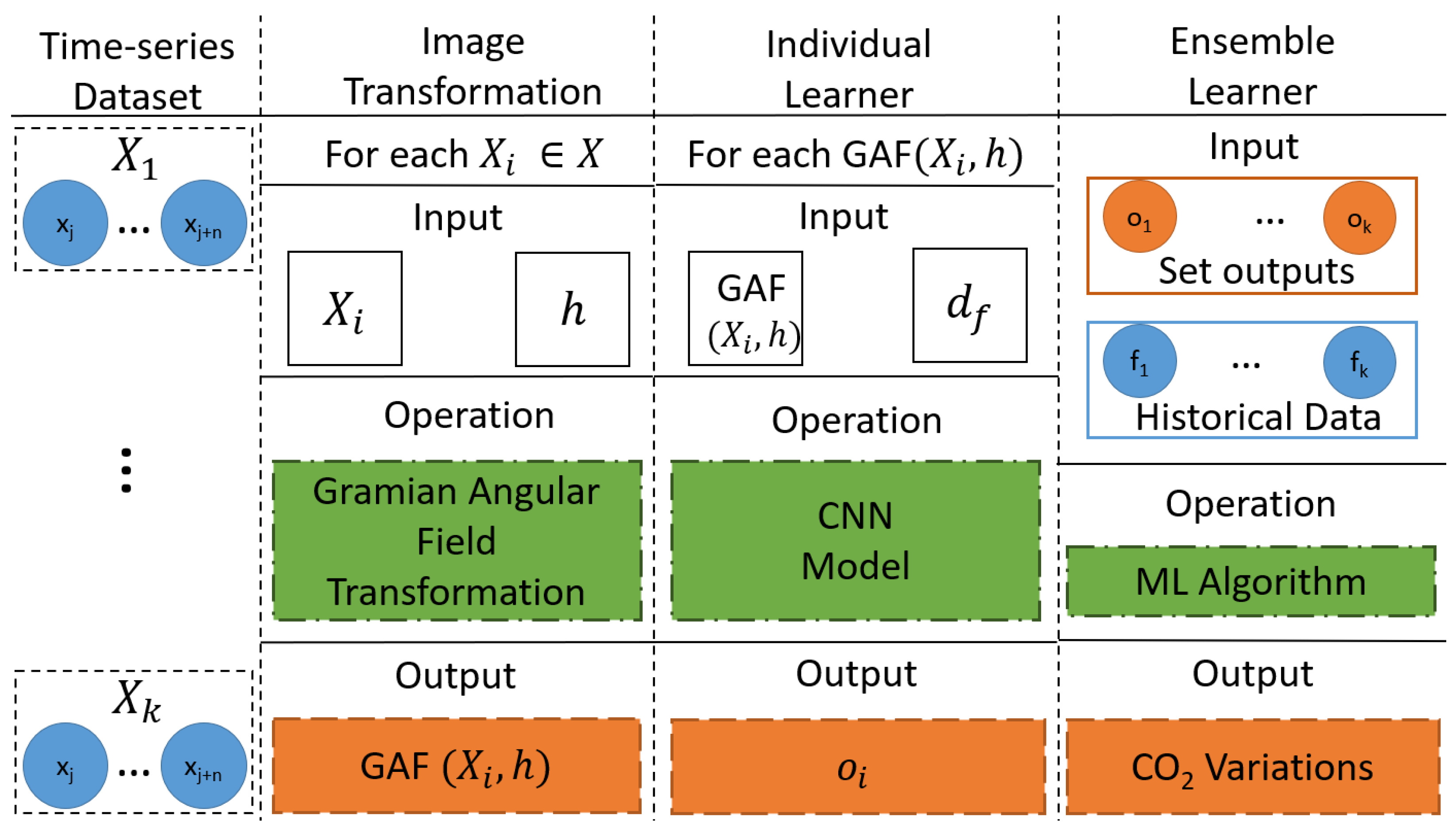
This section describes the steps applied to obtain accurate predictions of the variations in CO2 concentrations over a future time window. Figure 2 depicts the methodology referred to as the HMCOVP, such that each practical step is detailed based on the input to this step, the operation taking place, and its output. The following subsections explain each step of predicting CO2 variation direction and predicting CO2 variations. Time-series to Image Transformation and CNN Individual Learners are the building blocks to predict the CO2 future direction. Outputs of decreasing CO2 variation direction and ensemble learners are the foundations for CO2 variation predictions.
4.1. Time-Series to Image Transformation
The input represents time-series data of environmental features defined by , such that each where describes the time-series data of a single environmental feature. The discussion about the extracted environmental features is provided in the experimental setup. Accordingly, , such that n is the number of observations. To simplify the subsequent equations, would represent values of a feature i at timestamp j.
The exploratory data analysis showed that a lag time of up to 20 min for each environmental feature can be used to predict the CO2 concentration changes for a conference room that fits 12 people. As such, there is a need to reflect the existing time correlation in the feature engineering step. Python packages can be used for extracting time-based features such as the Time Series Feature Extraction Library [37] and Time Series FeatuRe Extraction on the basis of the Scalable Hypothesis test [38] (tsfresh). The extraction of hand-crafted features resulting from these two packages requires incorporating domain-specific insights, which are not available for the case under study. Additionally, the large feature space necessitates integrating feature selection or transformation steps. To address the limitations of the hand-crafted extraction of features, DNNs create their own features by the composition of multiple non-linear functions, each representing combinations of the input dataset features. One concern with DNNs, in their crude form, is their inability to model the time aspect, despite the manual process of including lagged versions of the features. Therefore, a feature engineering stage is incorporated to reflect the underlying time correlation between lagged versions of the available variables.
Wang and Oates [39] have devised the Gramian Angular Field (GAF) method for the transformation of time series data into a symmetrical 2D matrix. As opposed to other time series-to-image transformations, the resulting GAF image exposes the temporal dependencies between data points in a time series. Towards obtaining GAF images, two steps are followed. In the first step of the transformation, the time series data are normalized between . The normalization process is conducted in the following equation, whereby is the normalized value:
In the second step, the normalized data is transformed into the polar coordinate system that is calculated as follows:
After obtaining the transformation to polar coordinates for each data point, the next step is to generate a matrix that reflects the data dependencies between the new form of observations. The GAF technique exploits the angular representation by calculating the pairwise trigonometric sum between the points to reflect the temporal correlations. Considering a time frame of k seconds, such that , the GAF matrix is defined as follows:
The GAF matrix fits the requirements of the use case under study. First, it exposes the temporal dependencies present in the original time series as the time increases progressively from top-left to bottom-right. Second, the polar coordinates expose the relative correlations between data points with the help of superposition. Lastly, the time-series information is retained in the GAF matrix, which is beneficial when there is a need to integrate original data in any envisioned process. These original values can be extracted from the diagonal values. Each value in the GAF matrix is in the range of , which can be easily transformed into an image.
4.2. Individual Learners
The GAF images resulting from the time-series transformation process reflect the correlation by colour intensities. In their turn, these intensities translate the time correlation aspect of environmental sensory data through spatial resolution. CNNs, one of the variations of DNNs, are a strong candidate to find patterns in the produced grid-like structures and the output variable of concern. This selection stems from a CNN’s capability to infer spatial dependencies in a gird-structured input via its filters that extract specific features. Moreover, a CNN’s architecture is characterized by its sparse connections and weight sharing, which enables any developed model to be swiftly retrained and tested [40] compared to other resource-intensive and data-intensive DNN models such as LSTM. These properties are desirable for CNN models’ deployment in a resource-constrained and dynamically changing environment.
Predicting the variations in CO2 values is split into two steps. The first step is achieved using the individual learners considering the future direction of CO2 variations as its output variable. The direction is divided into three groups, decreasing equivalent to 0, increasing equivalent to 2, and constant equivalent to 1. The new definition of the output variables transforms the task at hand from regression to a classification task, which allows exploiting the wealth of literature for CNN-related classification tasks. The second step is achieved using the ensemble learner explained in the following sections.
A large body of research was conducted in the field of image recognition that experimented with different CNN architectures to obtain good accuracy results for their respective tasks. Therefore, a Transfer Learning (TL) approach is adopted to extract spatial features in the GAF representations to exploit these accumulated contributions. TL is a methodology to transfer the knowledge gained from an extensive source dataset to improve the learning process in the target dataset [41]. In DL, this methodology is implemented by transferring the weights learned from the source model to the target model. The differences between the source task, trained on the ImageNet dataset [42], and target tasks, trained on GAF representations, necessitate re-tuning the model’s weights using the target dataset or augmenting the initial model with extra layers so that the resulting model can accrue some of the characteristics of the target dataset. The employment of a TL approach has several benefits. The available pre-trained CNN models have proven their merit in a similar domain, saving the time needed to train and tune CNN models from scratch. The addition of more layers and consequently the exponential growth in the number of parameters are required to extract more abstract features from the input images. This step is integral for pattern recognition, which pre-conditions the existence of a large amount of data. The limitations of the deployment environment in terms of the constrained resources and gathered data drive the adoption of the TL approach.
The newly developed CNN model is built on each of the environmental features, such that the predictor of each variable is the feature’s GAF image for the history time window and the response variable is the direction of the variation of CO2 concentration levels for the future time window. The past and future time windows are denoted by h and f. Assuming that the CNN model is denoted by a function built on the data from the environmental feature , the predictor input GAF image by , and the prediction is , the created CNN model on the feature is as follows:
The following example is given to clarify the notation, the notions of history and future time windows, and the expression in general. If the current time is with a one-minute granularity, and the history and future time windows are 5 min for a feature , the GAF image represents values from to . The future time frame encompasses the values at and . Assuming that CO2 at is equal to 545 and CO2 and at is equal to 547, which means that .
4.3. Ensemble Learner
The dataset is split into training, validation, and testing sets. Models of each individual feature are developed using the training set. Since each individual learner outputs a probability prediction of each class, the probability of predicting decreasing change on the validation set is retained. This method is adopted to avoid overfitting the individual learners on the validation set. The individual learner’s classification task predicts the direction of future CO2 variations, instead of the variation itself. Therefore, the learner’s output probability values are combined with other features, describing the historical e2s values of each environmental feature, as inputs to an ensemble model to predict CO2 variations. This method is referred to as a Stacked Generalization ensemble. These features are obtained from the validation set. The set of outputs of all the individual features is denoted by such that represents the output of environmental feature i at the current time t. The set of historical features is defined as such that represents the historical environmental e2s values. The ensemble learner is denoted by . The predictors of the ensemble learner are represented by and the output is , such that p represents the variation of CO2 concentrations in , whereby w represents the future time window. The notation of the ensemble learner is as follows:
The exploratory data analysis has shown a varying correlation between CO2 values and the other environmental sensors. Because correlation values do not fully reflect the relationship between different environmental features, all the features were included in the Individual Learner step. This step yielded learners that are skillful in modelling the relationship between each environmental feature and the CO2 variation direction. However, since all of the features contribute to some extent to this variation, there is a need to reflect the relative importance of each model. Assigning weights based on the classification results is a method to convey the contribution of each model to the regression task. The environmental features’ predictions can be replaced by averaging the outcomes of each feature. However, this method does not explore the potential interactions existing between the input variables and undermines the classification of weak individual learners. Therefore, in this paper, different ensemble methods, representing supervised ML models, are explored and evaluated.
5. Experimental Setup
This section discusses the experimental procedure, which explains the different steps undertaken to solve the issue under study. After that, details of the implementation procedure are outlined and the evaluation criteria are investigated.
5.1. Experimental Parameters
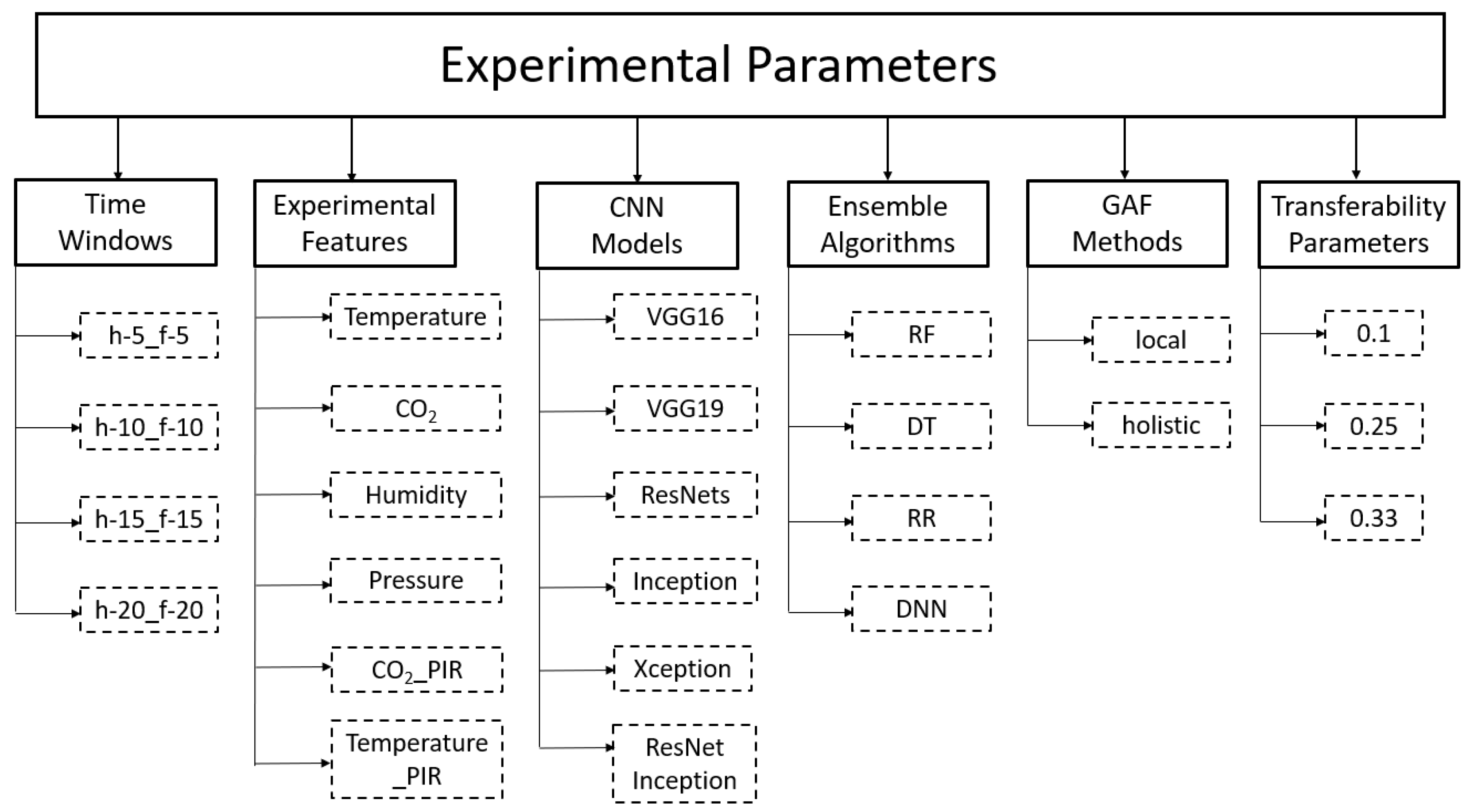
The analysis of HMCOVP commences by applying it to a large conference room, referred to as room00 and then later the models are evaluated on a smaller conference room, referred to as room01. Room00 can fit 12 people, with an area comprising 28.0 m2 and a volume of 89.6 m3 while room01 is of area 14.2 m2 and a volume of 38.3 m3 [25]. This process is followed to evaluate the transferability of the developed models to a room of different capacities. The hierarchical structure of HMCOVP promotes its transferability, which addresses a common concern in the IAQ-related literature. The following paragraphs explain the parameters involved in the experimental procedure summarized in Figure 3.
History and Future Time Windows: The EDA highlighted the relationship between lagged environmental features and the CO2 concentrations to infer a reasonable prediction time window. This EDA showed that a prediction horizon of 20 min is viable for the available dataset. The analysis includes the results of applying HMCOVP with the same time window for history and future time horizons. These parameters are subsets of the ones evaluated in FECOP. The remainder of the possible combinations will be considered in future work, given that the current formulation is not concerned with the memory constraints of the deployment environment. The history and the future time horizon will be referred to as “h-{w}_f-{w}”, whereby w represents the time window. Time windows of 5, 10, 15, and 20 min were considered. The combinations of the history and future time windows experimented with are h-5_f-5, h-10_f-10, h-15_f-15, and h-20_f-20.
The time series to image transformation step yielded several datasets that vary depending on the historical and future time windows. A 1-min sliding window is implemented to produce larger datasets. For example, for h-5_f-5, a single row is formed by predictors representing GAF images from to and the CO2 variations from to . The next row would represent the GAF images from to and the CO2 variations from to . The resulting process yields datasets of different sizes that range between 328,647 to 334,677 data points for training data and 74,085 to 74,730 data points for testing data for different history and future time horizons. The training and testing data points for different history and future time windows are summarized in Table 1.
Experimental Features: The original dataset consists of five environmental features: pressure, temperature, humidity, CO2 concentration, and activity levels. The activity level or PIR is a categorical variable formed of 0.5 increments from 0 to 12, amounting to 25 variables. The PIR feature space is first reduced to four categories, each representing eight contiguous activity levels, except 0, which is a category on its own. The one-hot encoding schema would create many 0–1 variables, which cannot be transformed into an image representation. Therefore, the PIR feature is transformed into two features, denoted by temperature_PIR and CO2_PIR. These two features are chosen because they exhibit the highest correlation with the PIR feature. The quantities are obtained by calculating the ratio of CO2 and temperature to the PIR feature. Six environmental features are obtained following this feature engineering step that includes CO2, temperature, pressure, humidity, CO2_PIR, and temperature_PIR.
GAF Representation: Normalization is a fundamental step in the time series to image transformation. Two main methods can branch out from this step, referred to as “local” and “holistic” approaches. Each of these methods targets a specific angle of the studied phenomenon. On the one hand, the “local” method calculates the minimum and the maximum in a defined w. This representation accentuates the small differences in such windows, reflected by the colour intensities of the GAF representation. On the other hand, the “holistic” approach calculates the minimum and the maximum over the whole datasets of a single environmental feature. The resulting GAF images are in concert with the dynamics in the whole dataset, which means that the images’ colour intensities mirror the differences in values in a w compared to value differences over the whole dataset. Both of these approaches are investigated in the experimental procedure. The existence of outliers is fundamental in the GAF representation, affecting the accuracy of CO2 variation predictions.
The EDA provided interesting insights into each environmental feature. Features such as CO2, CO2_PIR, and humidity displayed highly skewed distributions with large differences between the minimum and maximum values, to the detriment of the “holistic” approach. If these features are normalized based on these extremes, the majority of the data will fall within a small margin, and the resulting differences in GAF images will be minuscule. As a result, the CNNs will fail to infer any meaningful relationship from the GAF representation. A log transformation is applied to these features to mitigate the effect of outliers and to shrink the values’ ranges. Other features, such as pressure and temperature features displayed little variations. The exponential function is applied to each of these features to amplify these small differences. These concerns are not shared with the “local” approach, since its GAF representation depends on the minimum and maximum calculated in a time window. Therefore, the differences in feature values will be mirrored in the GAF representation despite their value ranges resulting from any transformation.
Individual CNN Models: The research community provides ample image recognition models for individual learners that can be applied to the generated datasets. These pre-trained CNN models include VGG16 and VGG19 [43], ResNets [44], ResNet_inception [45], Inception [46], and Xception [47] with different respective architectures. The experimental procedure evaluated all these CNN models. Keen readers can find the details of their respective architectures in the papers listed with every CNN model. Each of their architectures includes many convolutional and Fully Connected Layers (FCL). In the experimental procedure, the last layer that outputs the classification result is removed, given that a different dataset with different outputs is used in this study. Therefore, the remainder of the layers is augmented with a global average pooling layer and Fully Connected Layers (FCL). The obtained CNN models include either no FCLs, one FCL, or two FCLs. The number of neurons of these FCLs ranges from 64 to 4096 neurons.
Ensemble Learner Algorithms: Different algorithms were evaluated for the ensemble learning step. In particular, the same algorithms used in FECOP were evaluated following HMCOVP. These ML algorithms include RF, DT, RR, and DNNs. This step is followed to emphasize the distinction between the two methodologies in terms of the validity of feature engineering techniques.
Transferability Parameters: The transferability of the developed models is evaluated by applying them to a small room, denoted by room01, that fits two people. When the results were unsatisfactory, part of the training data of the target room is used to tune the parameters of the source room’s model. The fraction of the used training data is . Moreover, this experimental analysis included re-tuning or re-training the ensemble learners. Future works will include a more profound evaluation of the HCOMVP transferability.
5.2. Experimental Procedure
In the training phase of the methodology, the dataset is split into training, validation, and testing datasets. The training dataset is used to train the individual learners. The validation dataset is used to obtain the outputs of each of the individual learners that are used with the historical e2s values of environmental features in the validation set as inputs to train the ensemble learners. Such a split is followed to avoid overfitting the ensemble learner if fed with the outputs of the individual learners applied to the training set. After obtaining the trained individual learners and the ensemble learner, these learners are evaluated on the testing set.
5.3. Evaluation Metrics
The HMCOVP is evaluated against FECOP [30] and 1D CNNs, a popular method for time-series prediction. Since the problem of predicting CO2 variation prediction is a regression task, multiple evaluation metrics such as Mean Square Error (MSE) or Mean Absolute Error (MAE) can be used. Choosing one of these metrics depends on the experiments’ main goals.
The MSE metric emphasises the large errors while minimizing the effect of the smaller ones. On the other hand, the MAE equalises the effect of all individual errors. No anomaly detection method was applied to sanitize the gathered data, which suggests the existence of data corrupted with noise. This noise originates either from the environment itself or from the inaccuracies of the sensing technologies. Such circumstances call for a robust evaluation metric that can offset the noise’s effect. On a different note, the small prediction errors that are continually produced by models can result in long-term consequences to the HVAC systems. The predictions of CO2 variations affect the ventilation systems that need to maintain the indoor CO2 concentrations within acceptable levels and the estimation of current occupancy changes dictating the HVAC system’s operation. Consequently, small deviations, while insignificant in the short term, can accumulate unnecessary activation of HVAC systems, increasing the building’s Carbon footprint and energy expenditure. Large deviations of predictions originate either from models’ under-fitting data, which can be identified if it is a shared trend among different input values or from the existence of anomalous data that the model fails to fit. The anomalous data can be manifested by wrong sensor readings, corrupting the data with noise, or the occurrence of rare events that have little implications on long-term energy expenditure. As such, the robustness requirement and the equal importance of small and large deviations favour the use of MAE as an evaluation metric.
The MAE evaluation metric is used to find the best set of hyper-parameters on the validation set and to compare the performance of the HMCOVP, FECOP, and 1D CNNs on the testing set. The methods are evaluated on a set of CO2 variations exceeding pre-defined thresholds, including . These thresholds unveil different methods’ capability to predict big variations in CO2 concentration, which can potentially activate the HVAC systems and determine the instantaneous energy expenditure. The average MAE combining all these thresholds is employed to highlight the performance differences between the proposed methodology and the other approaches, providing a comprehensive overview of the proposed methods’ performance under different circumstances. The training and instance-wise testing times are incorporated into the evaluation to gauge the methods’ ability to learn in resource-constrained environments. Different CO2 variation thresholds and execution times are important factors of the deployment of proper solutions for building operators. The accurate predictions of CO2 changes are envisioned to facilitate the ventilation system’s decision-making processes. Therefore, the reduction in the superfluous activation of these systems translates into limiting energy expenditure. In the grand scheme of things, this methodology contributes to the mitigation of Carbon emissions, which can be quantified depending on the ore used for electricity production.
5.4. Implementation
The different algorithms used throughout this paper were built using sklearn [48] and Keras [49] python libraries. The developed models were evaluated on Windows 10 PC with a 3.00 GHz 24-Core AMD Threadripper processor, 128 GB of RAM, and 8 GB Nvidia GeForce RTX 3060 Ti GPU. The code is made available on the GitHub repository (https://github.com/Western-OC2-Lab/hierarchical-CO2, accessed on 14 May 2023).
6. Results and Discussion
This section analyses and discusses the results obtained from applying the HMCOVP. Firstly, it compares the performance of the HMCOVP using different parameters over different combinations of history and future time windows. After that, the best parameters are evaluated against competing methodologies. Lastly, the transferability of the models is investigated when applied to a smaller conference room.
6.1. Parameter Selection
Under different history and future time windows, this subsection explains the effect of parameters, including the GAF representation method, CNN models and their hyper-parameters, and ensemble learners. To that end, a subset of 10,000 data points for each history and future window combination (h&f) are used for parameter selection. A trial-and-error approach is conducted to find a subset that can balance training and evaluation times and underfitting avoidance. All the combinations of features were evaluated using a Grid Search method. More profound and less time-demanding approaches [50] will be investigated in future work. The sample of 10,000 data points is split into training, validation, and testing sets following the explained experimental procedure. Since many parameters are involved in the parameter selection procedure, this section explains a subset of these experiments. Keen readers and practitioners can refer to the code available through the GitHub repository for a comprehensive overview of the obtained results and the effect of all parameters. As such, the analysis in this section is restricted to the effect of different ensemble learners, the h&f combinations, and CO2 variation thresholds on the performance of the HMCOVP.
Table 2 summarises the findings of the parameter selection grouped by h&f. The best-performing combination of parameters and hyper-parameters with respect to each h&f are highlighted in bold. To highlight the significance of these differences in the MAE, it is important to map the obtained MAE values to their physical representations. The CO2 variation predictions help the ventilation systems in their decision-making process. Therefore, as previously mentioned, small MAEs can accumulate to falsely trigger the ventilation system. Moreover, less accurate CO2 variation predictions imply inaccurate prediction of the current effect of occupants and ventilation systems on CO2 concentration variations. Both of these factors contribute to reflecting an imprecise image of the environment in the HVAC decision-making systems. Accordingly, HVAC systems can be activated either early or late, contributing to potential violations of indoor environmental requirements and an increase in energy expenditure. As such, the MAE reflects a fundamental aspect of the HVAC system operation.
The variants of decision trees are the best-performing algorithms, represented by DT and RF. This shows that the non-linearity defines the relationship between the individual learners’ predictions and the historical e2s environmental features manifested through the superior MAE of non-linear algorithms (NN, RF, and DT) compared to the RR algorithm. The expansion of the prediction window contributed to a systematic increase in the MAE for all algorithms. This consensus is broken by the RF algorithm such that its MAE value decreases when the prediction horizon increases from 15 to 20 min. However, with more runs to execute, this exception will be reversed to conform to the trend. This increase in MAE is expected with the expansion of the future time window, given the increased probability of uncertainties affecting the environment, including the CO2 concentrations. In terms of the GAF representation, the best-performing models for each h&f combination do not highlight a preferable method. However, most ensemble learners display a better performance with the local method. Therefore, the CNN models extract representative information of CO2 variation direction with better accuracy when fed with GAF representations that accentuate local differences within a time window.
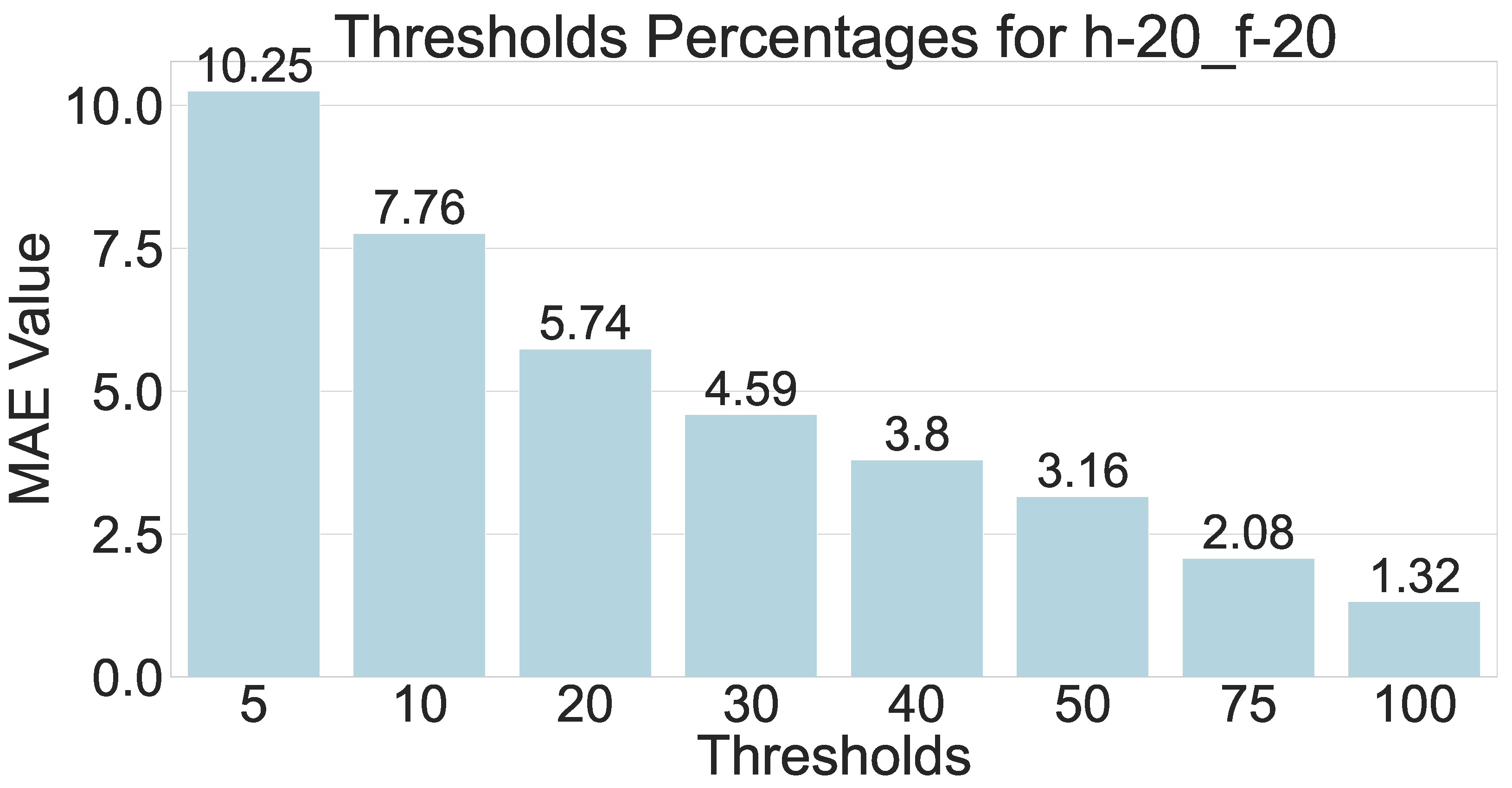
The summarized results in Table 2 have shown some parameter combinations that clearly outperform others. However, a clear limitation of the MAE parameter in this application is that it is skewed toward the values that constitute the majority of the response variable. In order to clarify this caveat, Figure 4 shows the percentage distributions of different absolute values of thresholds defined in the evaluation criteria. These results suggest that more than 60% of the variations are under 5 ppm. Therefore, a model with a low MAE is not fully representative of its performance on drastic changes in data. These radical changes are of higher importance for HVAC systems and building operators, but they are less common in the studied dataset. As a result, the crude MAE is replaced by a metric that averages the MAEs over each of the defined thresholds. This new metric is referred to as Thresh_MAE.
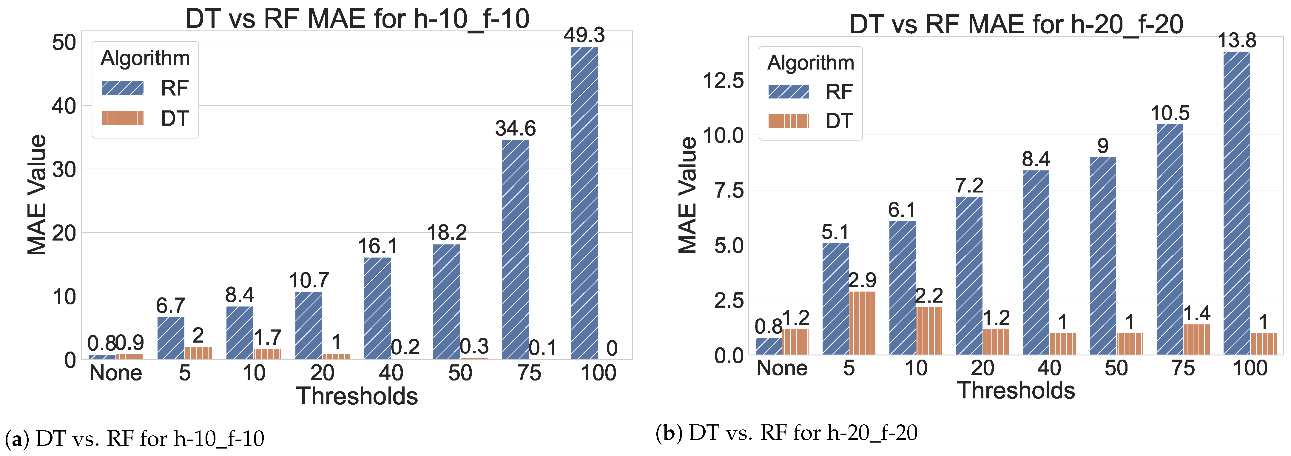
Figure 5 shows the differences in MAE for each of the defined thresholds for the two best-performing models in Table 2 that use DT or RF for ensemble learning. Figure 5a shows that RF combined with the other parameters included in Table 2 outperforms its DT counterpart when no thresholds are imposed. However, the performances start to diverge with increasing thresholds until a huge gap in performance is prominent. This trend shows that the RF model performs well on small variations in CO2 while DT outperforms RF when more drastic changes are involved. A similar observation can be applied to Figure 5b, whereby DT outperforms RF when thresholds are considered. However, a notable separation exists between the results of the RF for higher thresholds with the expansion of the prediction time horizon. This discrepancy is attributed to the abundance of more extreme variations with the expansion of future time windows. This fact enables the models to better map the relationships between these extreme values and the input variables, manifested by the lower MAE for higher thresholds.
Following the newly defined metric, Thresh_MAE, the best-performing parameters are shown in Table 3. As opposed to pure MAE, DT clearly outperformed all other ensemble learners and showed superior performance in predicting drastic variations. This observation is demonstrated by the decrease in Thresh_MAE value compared to MAE value, when DT is involved, for all h&f combinations. All the CNN models included FCLs, which emphasize the existing distinction between the source and target datasets in terms of the interactions between the extracted CNN features. Lastly, the local method of GAF representation dominates the better-performing combinations. This result shows that CNNs produce more informative features for CO2 direction prediction when the effect of small differences in values are magnified, resulting in more accurate classifications. The parameters included in Table 3 qualify for the next stage in the evaluation pipeline by training them on the whole training data and evaluating their performance on the testing test. The small Thresh_MAEs obtained in Table 3 unveil that the models overwhelmingly captured the factors affecting the environment. However, these small differences show that some environmental conditions are not considered, potentially playing a role in deciding the future variations in CO2 concentrations. These conditions may include the uncertainty of the environment that can be challenging to incorporate. Another factor can be connected to the interpolation strategy that is not reflective of the environmental dynamics. Lastly, the effect of the ventilation systems’ activation is excluded from the gathered data. This condition can affect the dynamics of the CO2 variation in connection with other environmental features.
6.2. HMCOVP vs. FECOP vs. 1D CNN
Table 4 summarises the performance of the three methods, our proposed methodology HMCOVP, FECOP, and 1D CNN, which are evaluated using Thresh_MAE and their training times. The best-performing combination configurations of hyper-parameters for the FECOP and 1D CNN are applied to the testing set. Similarly, the HMCOVP was implemented using the configurations outlined in Table 3. The HMCOVP significantly outperforms the other two methods in the prediction of the future CO2 variations in all the h&f combinations. The results prove the GAF images are better representatives of the time correlation aspects than the local features extracted by the 1D CNN to reflect these correlations. Additionally, the combination of image representations and numerical features present in the HMCOVP outperforms the rigorous feature engineering process of FECOP. While the HMCOVP incorporates some of the FECOP features, the distinctive quality of the features obtained from CNN models contributed to its superior performance. In some way, the HMCOVP combines the numeric features extracted in the FECOP and the time correlation found in the 1D CNN approach. These results prove the significance of hierarchical modelling.
The training times highlight salient differences between the methods. The 1D CNN method training time decreases with the expansion of the time window. This trend is expected given that fewer data are available for training when this happens. On the other hand, this trend is reversed for the FECOP. This phenomenon can be attributed to the feature engineering step, which extracts lagged versions of each environmental feature. As such, more features are extracted with the expansion of the time window, contributing to an increase in training time. Lastly, the HMCOVP does not exhibit any trend with the changes in the time window. Different configurations with varying model complexities contribute to the non-uniformity of training times. Compared to the FECOP and 1D CNN, the HMCOVP takes significantly more time to train given that it requires training six DL models and one ensemble model. The training of individual models can be executed in parallel, which significantly reduces the total training time. Therefore, a tradeoff exists between training times and the accuracy of the developed models.
6.3. Transferability Assessment
After proving its superior performance in predicting CO2 variations in room00, the next stage assesses the transferability of the developed models by applying them to a smaller room, referred to as room01, which only fits two people. The FECOP models’ results are obtained by training the models on the training set of room01. Both the HMCOVP and FECOP approaches are evaluated on the testing set of room01 using the Thresh_MAE metric. The evaluation criteria include the testing time per instance to infer the computational footprint of these methods. As for the HMCOVP, the models developed using room00’s training data are applied to the testing data of room01 without fine-tuning any of its individual learners or ensemble learner. As such, the transferability of the developed models is assessed in different spatial settings.
Table 5 summarises the results of the outlined process. In terms of predictive performance, the untuned HMCOVP outperforms its counterpart in every h&f combination. The HMCOVP models performed best with the h-15_f-15 and h-20_f-20 compared to other combinations. The h-15_f-15 combination performed best in terms of its Thresh_MAE, breaking the established trend of increasing Thresh_MAE with the increase in the prediction horizon. The h-20_f-20 experienced the least performance percentage gap in Thresh_MAE from room00 to room01. This observation means that the larger room’s environment dynamics acquired through hierarchical modelling closely resemble those of the smaller room in the bespoke combinations. As for smaller prediction horizons, it is expected that smaller rooms would exhibit different variations. In fact, changes in the small room’s environment, such as the existence of occupants, can momentarily affect the CO2 concentrations as opposed to the more spacious rooms. Lastly, the differences in the capacities of both rooms result in changes in the ranges of activity level-related features; thus, affecting the HMCOVP models’ accuracy. Consistent with the previous analysis, the FECOP approach is a less time and resource-intensive approach, manifested by its lower per-instance testing time. A 6–7× speedup is obtained by the FECOP approach; however, at the expense of its underwhelming prediction performance. The speedup benefit is blurred when the individual learners’ are parallelised.
The differences in feature scales between the two rooms require incorporating some of these missing characteristics into the developed HMCOVP model. Thanks to the hierarchical structure of the HMCOVP, the induction of this novel information can be realized on the level of individual and ensemble learners. As a result, the next step can include one of these scenarios. The first scenario re-tunes the individual CNN models by freezing some layers and training others. The second scenario replaces the old ensemble trained on room00 training data with a newer one trained using room01’s training data. While both scenarios are viable, choosing one of them depends on the obtained results and the nature of the data. The results have shown that the greatest performance divergence occurs in the ensemble learning phase as the individual learners almost produce the same accuracy results in both rooms. This gap can be surmised by the differences in e2s values and their effect on the future CO2 variations. Therefore, the ensemble learners are retrained using a subset of room01’s training data and evaluated using its testing data.
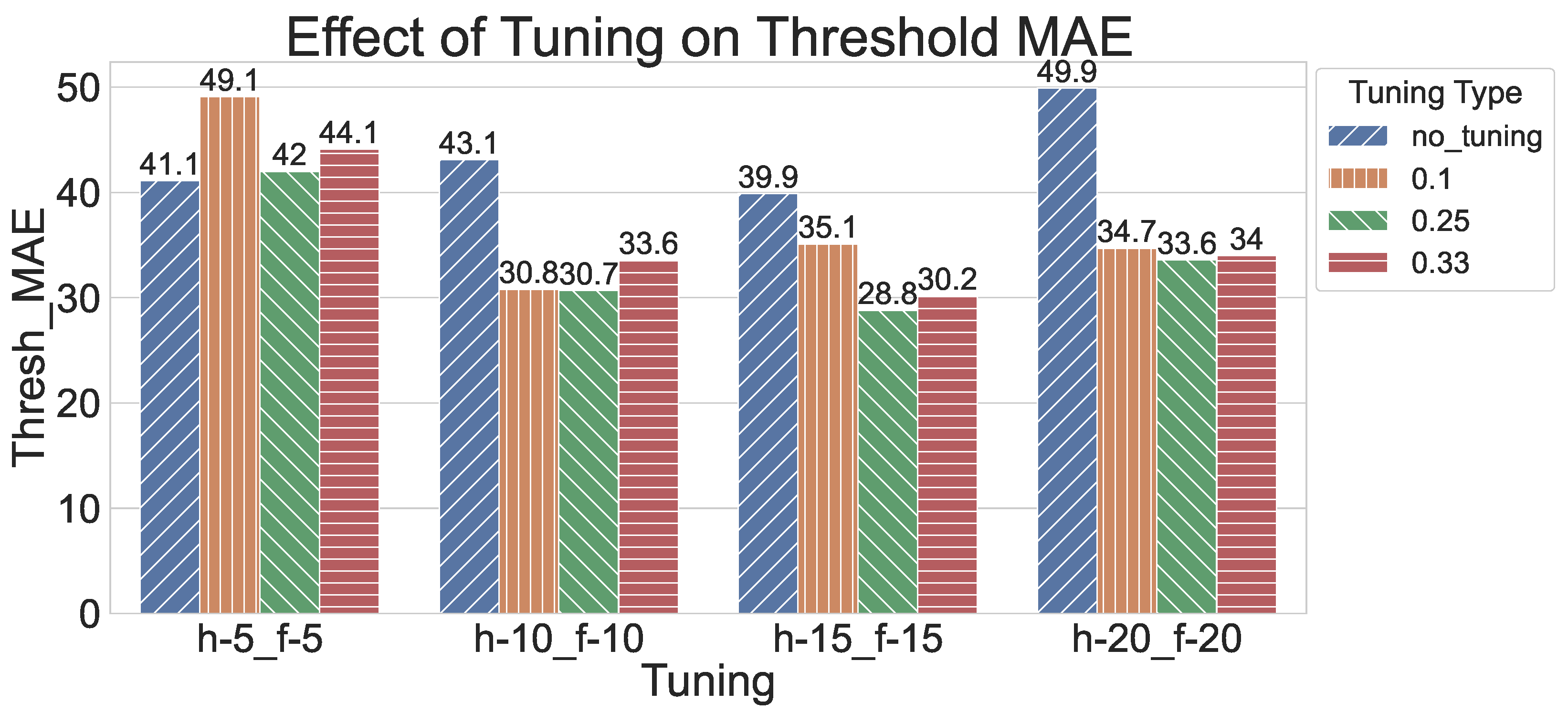
Figure 6 shows the effect of retraining the ensemble learner with different training sizes. The HMCOVP’s retrained ensemble model regressed in performance when applied to the h-5_f-5 combinations, regardless of the integrated training set’s size. This observation essentially suggests that the tuning process for this combination should incorporate individual models. On the other hand, a significant performance improvement is noted for all the other combinations. The greatest improvement is observed for the h-20_f-20 combinations, whereby its performance is the closest to the model applied to room00. For all the improved combinations, retraining the ensemble model with a quarter of the training set yields the best results. The results of these combinations show that incorporating the historical numerical values with the individual learners’ outputs contributes to performance enhancement. However, this alteration does not fully capture the dynamics of the target set, representing the small conference room. To mitigate the performance gap in CO2 variation predictions, the individual learners should be tuned the same as the ensemble learner. This aspect will be addressed in future work.
7. Conclusions
Buildings are one of the main contributors to energy consumption, whereby HVAC systems represent a controllable energy consumer. Specifically, ventilation systems are activated based on the requirements and existence of occupants. Therefore, the prediction of occupants and the utility of current ventilation control can be achieved through accurate predictions of proxy indicators, CO2 concentration changes, in particular, are key to the optimization of HVAC systems. This work proposes a hierarchical modelling approach, termed the HMCOVP, with the goal of accurately predicting CO2 concentration changes. The HMCOVP incorporates the time aspect by creating image-based lagged environment features and a hierarchical structure that enables the transferability of the developed models. These two features are missing in the state-of-the-art approaches. The HMCOVP was evaluated using a host of history and future time windows in a large office room and outperformed the state-of-the-art approaches by 400% using the mean absolute error metric. The transferability of the HMCOVP is investigated by applying and re-tuning the developed models in a smaller room and promising results are obtained. Overall, the HMCOVP successfully predicted future CO2 concentration changes in different spatial settings, facilitating the decision-making process of ventilation systems. Future work will experiment with ways to shorten the training time of the HMCOVP using feature selection techniques and enhance the transferability performance.
Author Contributions
Conceptualization, I.S. and A.S.; methodology, I.S.; software, I.S.; validation, I.S. and A.S.; formal analysis, I.S.; investigation, I.S.; resources, I.S.; data curation, I.S.; writing—original draft preparation, I.S.; writing—review and editing, I.S. and A.S.; visualization, I.S.; supervision, A.S.; project administration, A.S.; funding acquisition, A.S. All authors have read and agreed to the published version of the manuscript.
Funding
This research received no external funding.
Institutional Review Board Statement
Not applicable.
Data Availability Statement
The data presented and used in this study are openly available in Zenodo at (10.5281/zenodo.3774723).
Conflicts of Interest
The authors declare no conflict of interest.
References
- The Rockefeller Foundation and Deutsche Bank Group. Building Retrofit Paper—Final 3-1-12 vEDIT. Rockefellerfoundation. Available online: https://www.rockefellerfoundation.org/wp-content/uploads/United-States-Building-Energy-Efficiency-Retrofits.pdf (accessed on 16 May 2020).
- Berardi, U. Building energy consumption in US, EU, and BRIC countries. Procedia Eng. 2015, 118, 128–136. [Google Scholar] [CrossRef]
- Pérez-Lombard, L.; Ortiz, J.; Pout, C. A review on buildings energy consumption information. Energy Build. 2008, 40, 394–398. [Google Scholar] [CrossRef]
- Satish, U.; Mendell, M.J.; Shekhar, K.; Hotchi, T.; Sullivan, D.; Streufert, S.; Fisk, W.J. Is CO2 an indoor pollutant? Direct effects of low-to-moderate CO2 concentrations on human decision-making performance. Environ. Health Perspect. 2012, 120, 1671–1677. [Google Scholar] [CrossRef] [PubMed]
- Du, B.; Tandoc, M.C.; Mack, M.L.; Siegel, J.A. Indoor CO2 concentrations and cognitive function: A critical review. Indoor Air 2020, 30, 1067–1082. [Google Scholar] [CrossRef]
- Lewis, D. Why indoor spaces are still prime COVID hotspots. Nature 2021, 592, 22–25. [Google Scholar] [CrossRef] [PubMed]
- Berry, G.; Parsons, A.; Morgan, M.; Rickert, J.; Cho, H. A review of methods to reduce the probability of the airborne spread of COVID-19 in ventilation systems and enclosed spaces. Environ. Res. 2022, 203, 111765. [Google Scholar] [CrossRef]
- World Health Organization. A Conceptual Framework for Action on the Social Determinants of Health; World Health Organization: Geneva, Switzerland, 2010. [Google Scholar]
- Xin, J.; Duan, Q.; Jin, K.; Sun, J. A reduced-scale experimental study of dispersion characteristics of hydrogen leakage in an underground parking garage. Int. J. Hydrogen Energy 2023, 48, 16936–16948. [Google Scholar] [CrossRef]
- Mallach, G.; St-Jean, M.; MacNeill, M.; Aubin, D.; Wallace, L.; Shin, T.; Van Ryswyk, K.; Kulka, R.; You, H.; Fugler, D.; et al. Exhaust ventilation in attached garages improves residential indoor air quality. Indoor Air 2017, 27, 487–499. [Google Scholar] [CrossRef]
- Cao, S.; Chen, X.; Zhang, L.; Xing, X.; Wen, D.; Wang, B.; Qin, N.; Wei, F.; Duan, X. Quantificational exposure, sources, and health risks posed by heavy metals in indoor and outdoor household dust in a typical smelting area in China. Indoor Air 2020, 30, 872–884. [Google Scholar] [CrossRef]
- Liao, W.; Liu, X.; Kang, N.; Song, Y.; Wang, L.; Yuchi, Y.; Huo, W.; Mao, Z.; Hou, J.; Wang, C. Associations of cooking fuel types and daily cooking duration with sleep quality in rural adults: Effect modification of kitchen ventilation. Sci. Total Environ. 2023, 854, 158827. [Google Scholar] [CrossRef]
- Cakyova, K.; Figueiredo, A.; Oliveira, R.; Rebelo, F.; Vicente, R.; Fokaides, P. Simulation of passive ventilation strategies towards indoor CO2 concentration reduction for passive houses. J. Build. Eng. 2021, 43, 103108. [Google Scholar] [CrossRef]
- Metcalf, G.E.; Weisbach, D. The design of a carbon tax. Harv. Environ. Law Rev. 2009, 33, 499. [Google Scholar] [CrossRef]
- Act, E.P. Energy Policy Act of 2005; US Congress: Washington, DC, USA, 2005.
- Esrafilian-Najafabadi, M.; Haghighat, F. Occupancy-based HVAC control systems in buildings: A state-of-the-art review. Build. Environ. 2021, 197, 107810. [Google Scholar] [CrossRef]
- Kleiminger, W.; Mattern, F.; Santini, S. Predicting household occupancy for smart heating control: A comparative performance analysis of state-of-the-art approaches. Energy Build. 2014, 85, 493–505. [Google Scholar] [CrossRef]
- Zou, H.; Zhou, Y.; Yang, J.; Spanos, C.J. Towards occupant activity driven smart buildings via WiFi-enabled IoT devices and deep learning. Energy Build. 2018, 177, 12–22. [Google Scholar] [CrossRef]
- Scislo, L.; Szczepanik-Scislo, N. Air quality sensor data collection and analytics with iot for an apartment with mechanical ventilation. In Proceedings of the 2021 11th IEEE International Conference on Intelligent Data Acquisition and Advanced Computing Systems: Technology and Applications (IDAACS), Cracow, Poland, 22–25 September 2021; Volume 2, pp. 932–936. [Google Scholar]
- Sun, K.; Zhao, Q.; Zou, J. A review of building occupancy measurement systems. Energy Build. 2020, 216, 109965. [Google Scholar] [CrossRef]
- Naylor, S.; Gillott, M.; Lau, T. A review of occupant-centric building control strategies to reduce building energy use. Renew. Sustain. Energy Rev. 2018, 96, 1–10. [Google Scholar] [CrossRef]
- Chen, Z.; Jiang, C.; Xie, L. Building occupancy estimation and detection: A review. Energy Build. 2018, 169, 260–270. [Google Scholar] [CrossRef]
- Li, C.; Cui, C.; Li, M. A proactive 2-stage indoor CO2-based demand-controlled ventilation method considering control performance and energy efficiency. Appl. Energy 2023, 329, 120288. [Google Scholar] [CrossRef]
- Chen, Z.; Zhao, R.; Zhu, Q.; Masood, M.K.; Soh, Y.C.; Mao, K. Building occupancy estimation with environmental sensors via CDBLSTM. IEEE Trans. Ind. Electron. 2017, 64, 9549–9559. [Google Scholar] [CrossRef]
- Räsänen, P.; Koivusaari, J.; Kallio, J.; Rehu, J.; Ronkainen, J.; Tervonen, J.; Peltola, J. VTT SCOTT IAQ Dataset. 2020. Available online: https://zenodo.org/record/3774723#.ZGOobXbMKUk (accessed on 16 June 2022).
- Dong, B.; Andrews, B.; Lam, K.P.; Höynck, M.; Zhang, R.; Chiou, Y.S.; Benitez, D. An information technology enabled sustainability test-bed (ITEST) for occupancy detection through an environmental sensing network. Energy Build. 2010, 42, 1038–1046. [Google Scholar] [CrossRef]
- Candanedo, L.M.; Feldheim, V. Accurate occupancy detection of an office room from light, temperature, humidity and CO2 measurements using statistical learning models. Energy Build. 2016, 112, 28–39. [Google Scholar] [CrossRef]
- Masood, M.K.; Soh, Y.C.; Jiang, C. Occupancy estimation from environmental parameters using wrapper and hybrid feature selection. Appl. Soft Comput. 2017, 60, 482–494. [Google Scholar] [CrossRef]
- Shaer, I.; Shami, A. Sound Event Classification in an Industrial Environment: Pipe Leakage Detection Use Case. In Proceedings of the International Wireless Communications and Mobile Computing (IWCMC), Dubrovnik, Croatia, 30 May–3 June 2022; pp. 1212–1217. [Google Scholar]
- Kallio, J.; Tervonen, J.; Räsänen, P.; Mäkynen, R.; Koivusaari, J.; Peltola, J. Forecasting office indoor CO2 concentration using machine learning with a one-year dataset. Build. Environ. 2021, 187, 107409. [Google Scholar] [CrossRef]
- Golestan, S.; Kazemian, S.; Ardakanian, O. Data-driven models for building occupancy estimation. In Proceedings of the Ninth International Conference on Future Energy Systems, Karlsruhe, Germany, 12–15 June 2018; pp. 277–281. [Google Scholar]
- Stjelja, D.; Jokisalo, J.; Kosonen, R. Scalable Room Occupancy Prediction with Deep Transfer Learning Using Indoor Climate Sensor. Energies 2022, 15, 2078. [Google Scholar] [CrossRef]
- Wang, Z.; Hong, T.; Piette, M.A.; Pritoni, M. Inferring occupant counts from Wi-Fi data in buildings through machine learning. Build. Environ. 2019, 158, 281–294. [Google Scholar] [CrossRef]
- Laaroussi, Y.; Bahrar, M.; El Mankibi, M.; Draoui, A.; Si-Larbi, A. Occupant presence and behavior: A major issue for building energy performance simulation and assessment. Sustain. Cities Soc. 2020, 63, 102420. [Google Scholar] [CrossRef]
- Yu, L.; Sun, Y.; Xu, Z.; Shen, C.; Yue, D.; Jiang, T.; Guan, X. Multi-agent deep reinforcement learning for HVAC control in commercial buildings. IEEE Trans. Smart Grid 2020, 12, 407–419. [Google Scholar] [CrossRef]
- Wang, Y.; Velswamy, K.; Huang, B. A long-short term memory recurrent neural network based reinforcement learning controller for office heating ventilation and air conditioning systems. Processes 2017, 5, 46. [Google Scholar] [CrossRef]
- Barandas, M.; Folgado, D.; Fernandes, L.; Santos, S.; Abreu, M.; Bota, P.; Liu, H.; Schultz, T.; Gamboa, H. TSFEL: Time series feature extraction library. SoftwareX 2020, 11, 100456. [Google Scholar] [CrossRef]
- Christ, M.; Braun, N.; Neuffer, J.; Kempa-Liehr, A.W. Time series feature extraction on basis of scalable hypothesis tests (tsfresh–a python package). Neurocomputing 2018, 307, 72–77. [Google Scholar] [CrossRef]
- Wang, Z.; Oates, T. Imaging time-series to improve classification and imputation. In Proceedings of the Twenty-Fourth International Joint Conference on Artificial Intelligence, Buenos Aires, Argentina, 25–31 July 2015. [Google Scholar]
- Osaku, D.; Gomes, J.F.; Falcão, A.X. Convolutional neural network simplification with progressive retraining. Pattern Recognit. Lett. 2021, 150, 235–241. [Google Scholar] [CrossRef]
- Weiss, K.; Khoshgoftaar, T.M.; Wang, D. A survey of transfer learning. J. Big Data 2016, 3, 1–40. [Google Scholar]
- Deng, J.; Dong, W.; Socher, R.; Li, L.J.; Li, K.; Fei-Fei, L. Imagenet: A large-scale hierarchical image database. In Proceedings of the 2009 IEEE Conference on Computer Vision and Pattern Recognition, Miami, FL, USA, 20–25 June 2009; pp. 248–255. [Google Scholar]
- Simonyan, K.; Zisserman, A. Very deep convolutional networks for large-scale image recognition. arXiv 2014, arXiv:1409.1556. [Google Scholar]
- He, K.; Zhang, X.; Ren, S.; Sun, J. Deep residual learning for image recognition. In Proceedings of the IEEE Conference on Computer Vision and Pattern Recognition, Las Vegas, NV, USA, 27–30 June 2016; pp. 770–778. [Google Scholar]
- Szegedy, C.; Ioffe, S.; Vanhoucke, V.; Alemi, A.A. Inception-v4, inception-resnet and the impact of residual connections on learning. In Proceedings of the Thirty-First AAAI Conference on Artificial Intelligence, San Francisco, CA, USA, 4–9 February 2017. [Google Scholar]
- Szegedy, C.; Vanhoucke, V.; Ioffe, S.; Shlens, J.; Wojna, Z. Rethinking the inception architecture for computer vision. In Proceedings of the IEEE Conference on Computer Vision and Pattern Recognition, Las Vegas, NV, USA, 27–30 June 2016; pp. 2818–2826. [Google Scholar]
- Chollet, F. Xception: Deep learning with depthwise separable convolutions. In Proceedings of the IEEE Conference on Computer Vision and Pattern Recognition, Honolulu, HI, USA, 21–26 July 2017; pp. 1251–1258. [Google Scholar]
- Pedregosa, F.; Varoquaux, G.; Gramfort, A.; Michel, V.; Thirion, B.; Grisel, O.; Blondel, M.; Prettenhofer, P.; Weiss, R.; Dubourg, V.; et al. Scikit-learn: Machine Learning in Python. J. Mach. Learn. Res. 2011, 12, 2825–2830. [Google Scholar]
- Chollet, F. Keras. 2015. Available online: https://keras.io (accessed on 16 May 2023).
- Yang, L.; Shami, A. On hyperparameter optimization of machine learning algorithms: Theory and practice. Neurocomputing 2020, 415, 295–316. [Google Scholar] [CrossRef]
Figure 1.
Distribution of Correlations.

Figure 2.
Methodology Steps.

Figure 3.
Summary of Experimental Parameters.

Figure 4.
Thresholds’ Data Percentages.

Figure 5.
MAE for Different Thresholds.

Figure 6.
Effect of Tuning.


Table 1.
Dataset Sizes.
| History (Minutes) | Future (Minutes) | Training Data Testing Data |
|---|---|---|
| h-5 | f-5 | 334,677 74,730 |
| h-10 | f-10 | 332,667 74,514 |
| h-15 | f-15 | 330,657 74,300 |
| h-20 | f-20 | 328,647 74,085 |
Table 2.
Parameter Selection on the Training Dataset.
| History and Future Time Window (in Minutes) | Ensemble Algorithm | CNN Model | CNN FCL | Method | MAE |
|---|---|---|---|---|---|
| h-5_f-5 | RR | VGG_16 | [64] | holistic | 1.61 |
| DT | Resnet_152 | [256] | local | 0.65 | |
| RF | VGG_16 | [512] | holistic | 0.4 | |
| NN | Resenet_152 | [512, 256] | holistic | 1.3 | |
| h-10_f-10 | RR | VGG_19 | [4096] | local | 3.25 |
| DT | VGG_19 | [512] | local | 0.84 | |
| RF | Resnet_152 | [128, 64] | local | 0.765 | |
| NN | Resnet_101 | [256, 128] | local | 2.63 | |
| h-15_f-15 | RR | VGG_16 | None | local | 5.54 |
| DT | Resnet_152 | [256, 128] | local | 0.98 | |
| RF | Xception | None | local | 1.22 | |
| NN | Resnet_101 | [256] | local | 4.48 | |
| h-20_f-20 | RR | Resnet_50 | [128] | holistic | 6.07 |
| DT | Resnet_101 | [128, 64] | local | 1.18 | |
| RF | VGG_19 | [4096] | holistic | 0.84 | |
| NN | Resnet_50 | [128, 64] | local | 4.91 |
Table 3.
Best-Performing Combinations.
| h&f | Ensemble | CNN Model | CNN FCL | Method | Thresh_MAE |
|---|---|---|---|---|---|
| h-5_f-5 | DT | Xception | [512] | local | 0.11 |
| h-10_f-10 | DT | Resnet_50 | [128, 64] | local | 0.6 |
| h-15_f-15 | DT | Resnet_152 | [256, 128] | local | 1.0 |
| h-20_f-20 | DT | Resnet_101 | [128, 64] | local | 1.49 |
Table 4.
HMCOVP vs. FECOP vs. 1D-CNN.
| Parameter | Thresh_MAE | Training Time (min) | ||||
|---|---|---|---|---|---|---|
| Methodologies | HMCOVP | FECOP | 1D-CNN | HMCOVP | FECOP | 1D-CNN |
| h-5_f-5 | 10.14 | 40.89 | 2331.11 | 229.69 | 2.1 | 36.5 |
| h-10_f-10 | 14.48 | 52.52 | 8969.98 | 360.34 | 2.275 | 22.62 |
| h-15_f-15 | 19.37 | 66.83 | 9201.81 | 716.54 | 2.83 | 19.16 |
| h-20_f-20 | 27.74 | 77.21 | 10,128.83 | 381.78 | 3.62 | 17.84 |
Table 5.
Room01 Result Comparisons.
| Parameters | Thresh_MAE | Time/Instance (ms) | ||
|---|---|---|---|---|
| Methodologies | HMCOVP | FECOP | HMCOVP | FECOP |
| h-5_f-5 | 41.11 | 49.35 | 6.24 | 0.67 |
| h-10_f-10 | 43.14 | 52.4 | 6.48 | 1.14 |
| h-15_f-15 | 39.90 | 55.9 | 14.64 | 2.16 |
| h-20_f-20 | 49.93 | 54.2 | 10.44 | 1.44 |
Disclaimer/Publisher’s Note: The statements, opinions and data contained in all publications are solely those of the individual author(s) and contributor(s) and not of MDPI and/or the editor(s). MDPI and/or the editor(s) disclaim responsibility for any injury to people or property resulting from any ideas, methods, instructions or products referred to in the content. |
© 2023 by the authors. Licensee MDPI, Basel, Switzerland. This article is an open access article distributed under the terms and conditions of the Creative Commons Attribution (CC BY) license (https://creativecommons.org/licenses/by/4.0/).
Share and Cite
MDPI and ACS Style
Shaer, I.; Shami, A. Hierarchical Modelling for CO2 Variation Prediction for HVAC System Operation. Algorithms 2023, 16, 256. https://0-doi-org.brum.beds.ac.uk/10.3390/a16050256
AMA Style
Shaer I, Shami A. Hierarchical Modelling for CO2 Variation Prediction for HVAC System Operation. Algorithms. 2023; 16(5):256. https://0-doi-org.brum.beds.ac.uk/10.3390/a16050256
Chicago/Turabian StyleShaer, Ibrahim, and Abdallah Shami. 2023. "Hierarchical Modelling for CO2 Variation Prediction for HVAC System Operation" Algorithms 16, no. 5: 256. https://0-doi-org.brum.beds.ac.uk/10.3390/a16050256
Note that from the first issue of 2016, this journal uses article numbers instead of page numbers. See further details here.