1. Introduction
Lung cancer ranks as one of the most common causes of death amongst all diseases. While there have been a lot of approaches to minimize the fatalities caused by this disease, early detection is considered the best step towards effective treatment. The overall five-year survival rate for lung cancer is 14%. Nonetheless, patients at the early stage of the disease who undergo curative resection have a five-year survival rate of 40% to 70%. The most recent estimate statistics, according to the American Cancer Society, indicate that in 2014, there were 224,210 new cases, accounting for about 13% of all cancer diagnoses. Lung cancer accounts for more deaths than any other cancer in both men and women. An estimated 221,200 new cases of lung cancer are expected in 2015. Furthermore, an estimated 158,040 deaths are expected to occur in 2015, accounting for about 27% of all cancer deaths [
1].
The detection of lung cancer can be achieved in several ways, such as computed tomography (CT), magnetic resonance imaging (MRI), and X-ray. All these methods consume a lot of resources in terms of both time and money, in addition to their invasiveness. Recently, scientists have proven that the non-invasive technique of sputum cell analysis can assist in the successful diagnosis of lung cancer. A computer-aided-diagnosis (CAD) system using this modality would be of great support for pathologists when dealing with large amounts of data, in addition to relieving doctors from tedious and routine tasks. The design and development of sputum color image segmentation is an extremely challenging task. A part from the work reported in [
2], where the authors used Hopfield Neural Network (HNN) to classify the sputum cells into cancer or non-cancer cell, little or nothing has been done in developing a CAD system based on sputum cytology.
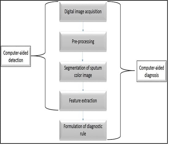
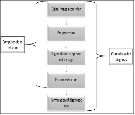
In this paper a state-of-the-art CAD system is implemented based on sputum color image analysis. The CAD system can play a significant role in early lung cancer detection. It serves as a useful second opinion when physicians examine patients during lung cancer screening [
3]. A CAD system involves a combination of image processing and artificial intelligent techniques that can be used to detect abnormalities in medical images as well as enhancing medical interpretation for a better performance in the diagnosis process. In addition, a CAD system could direct the pathologist’s attention to the regions where the probability of presence of the disease is greater [
4]. On the other hand, the major role of the CAD system is to improve the sensitivity of the diagnosis process and not to make decisions about the patient’s health status [
5]. The proposed CAD system was tested on 100 sputum color images for early lung cancer detection, the experimental results were substantially improved, with high values of sensitivity, specificity and accuracy, in addition to an accurate detection of the cancerous cells when compared with the pathologist’s diagnosis results. Therefore, the new CAD system could increase the efficiency of the mass screening process by detecting the lung cancer candidates successfully and improve the performance of pathology in the diagnosis process. The novelty of this work is defined as follows: a state-of-the-art complete CAD system is implemented based on the sputum color image analysis, and optimal deployment and combination of existing image processing and analysis techniques for building the computer aided diagnosis (CAD) system is used. The contributions can be summarized as follows: (1) Detection of sputum cell using a Bayesian classification framework; (2) Best color space after analysis of the images with histogram analysis; (3) Mean shift technique for the sputum cell segmentation; (4) Feature extraction, where a set of features are extracted from the nucleus region to be used in the diagnosis process. Based on medical knowledge, the following features were used in our proposed CAD system: Nucleus to Cytoplasm (NC) ratio, perimeter, density, curvature, circularity and eigen ratio; (5) Classification of sputum cells into benign or malignant cells is done by using different classification techniques: artificial neural network (ANN) and support vector machine (SVM).
The rest of the paper is organized as follows.
Section 2 provides the background to the existing methods of lung cancer diagnosis.
Section 3 describes sputum cells extraction and segmentation.
Section 4 presents the feature extraction.
Section 5 provides a detail description about the different classification methods.
Section 6 compares the proposed CAD system with other systems. Finally, the conclusion and future works are discussed in
Section 7.
2. Background
Lung cancer remains the leading cause of mortality. There is significant evidence indicating that the early detection of lung cancer will decrease the mortality rate, by using asymptomatic screening methods, followed by effective treatment. Most recent research relies on quantitative information, such as size, shape, and the ratio of the affected cells. Computer vision methods are employed to elicit information from medical images, such as the detection of cancerous cells. Many diagnostic ambiguities are removed when transforming these images from their continuous to their digital form. Today, very large amounts of data are produced from medical imaging modalities, such as sputum cytology, computed tomography (CT) and magnetic resonance imaging (MRI) [
6]. In the literature, there exists many modalities that have been used for detecting lung cancer, some of them can detect the cancer in early stages, and others can detect the cancer in advanced stages. Some of lung cancer modalities are: computed tomography (CT) scans, positron emission tomography (PET) data, X-ray images and sputum color image analysis.
The authors in [
7] used CT scans to detect histological images of the lungs and diagnose into cancerous or non-cancerous nodules. The segmentation process is done by using a fuzzy system based on the area and the gray level of the nodule region. These methods attain an accuracy of 90% with high values for sensitivity and specificity that can meet the clinical diagnosis requirement. Other authors [
8] used high resolution (HRCT) images to detect small lung nodules by applying a series of 3D cylindrical and spherical filters. The drawback was in the limitation of this method in detecting all cancerous nodules. Using CT scans in detecting lung cancer has a number of limitations with high false-positive rate, because it detects a lot of non-cancerous nodules and it misses many small cancer nodules.
The PET scan which is used in conjunction with X-rays or CT scans, is considered the most recent nuclear medicine imaging of the functional processes within the human body. The biggest advantage of a PET scan, compared to other modalities, is that it can reveal how a part of the patient’s body is functioning, rather than just how it looks. The author in [
9] proposed an automated process of tumor delineation and volume detection from each frame of PET lung images. The spatial and frequency domain features have been used to represent the data. K-nearest neighbor and support vector machines (SVM) classifiers have been used to measure the performance of the features. Wavelet features with a SVM classifier gave a consistent accuracy of 97% with an average sensitivity and specificity of 81% and 99%, respectively. The calculated volume from the detected tumor by the proposed method matched the manually segmented volume by physicians. Their methods succeeded in eliminating the need for manual tumor segmentation, thus reducing physician fatigue to a great extent, however the limitation of the PET scan is that it can be time consuming. It can take from several hours to days for the radiotracer to accumulate in the body part of interest. In addition, the resolution of body structures with nuclear medicine may not be as high as with other imaging techniques, such as CT.
The X-ray image, or chest radiography, is one of the most commonly used diagnostic modalities in lung cancer detection and is regarded as one of the cheapest diagnostic tools. The authors in [
10] proposed a nodule detection algorithm in chest radiographs. The algorithm consisting of four steps: image acquisition, image preprocessing, nodule candidate segmentation and feature extraction. Active shape model technique for lung image segmentation was used, while gray level co-occurrence matrix technique was adopted for texture features. The limitation can be in its invasive nature (patients’ radiation exposure), plus high false positive and negative rates.
The latest modality is sputum cytology, which has developed to become an important modality that can be used to detect early lung cancer. A number of medical researchers now utilize analysis of sputum cells for this early detection. The detection of lung cancer by using sputum color images was introduced in [
2] where, for the diagnosis, the authors presented unsupervised classification technique based on HNN to segment the sputum cells into cancerous and normal cells. They used energy function with cost term to increase the accuracy in the segmented regions. Their technique resulted in correct segmentation of sputum color image cells into nuclei, cytoplasm and clear background classes. However, the methods have limitations due to the problem of early local minima of the HNN. The HNN can make a crisp classification of the cells after removing all debris cells. The authors in [
11] overcame this problem by using a mask algorithm as a pre-processing step for removing all debris cells and classifying the overlapping cells as separate cells. They concluded that the HNN gives better classification results than other methods such as fuzzy clustering technique and can be used in the diagnosis process.
The author in [
12] used all the previous results to come up with an automatic computer aided diagnosis system for early detection of lung cancer based on the analysis of pathological sputum color images. Two segmentation processes were used, the first one was Fuzzy C-Means Clustering algorithm (FCM), and the second was the improved version of HNN for the classification of the sputum images into background, nuclei and cytoplasm. The two regions were used as a main feature to diagnose each extracted cell. It was found that the HNN segmentation results are more accurate and reliable than FCM clustering in all cases. The HNN succeeded in extracting the nuclei and cytoplasm regions. However, FCM failed in detecting the nuclei, instead detecting only part of it. In addition, the FCM is not sensitive to intensity variations as segmentation error at convergence is larger with FCM compared to that with HNN.
In the previous cases [
2,
11,
12], the detection of lung cancer was done through the analysis of sputum color images by applying data mining techniques such as clustering and classification followed by shape detection. However, the techniques which were used to analyze these images have a number of limitations namely: the high number of false negatives representing the missed cancer cells, and the high number of false positives representing cells classified as cancerous, resulting in putting a patient through unnecessary radiation and surgical operations. In addition, most techniques fail to consider the outer pixels which may sometimes represent a class in themselves. Moreover, the preprocessing techniques need further enhancement to discard the debris cells in the background of the images, and to remove all noise from the images, in addition to the overlapping between the sputum cells which have not been considered by the previous techniques.
The current segmentation results are not accurate enough to be used in the diagnosis part. In the HNN-based method, the cluster number has to be provided in advance. This affects the feature extraction part, especially in the presence of outliers. These problems have to be tackled, and more features have to be computed to develop a successful CAD system. Hence this leaves scope for further investigation of a method that detects the lung cancer in the early stage.
4. Feature Extraction
After detecting the nucleus and cytoplasm area in the cell, we extracted different features, which will be used in the diagnostic process for detecting the cancer cells. The main problem that faces any CAD systems for early diagnosis of lung cancer is associated with the ability of the CAD system to discriminate between normal and abnormal cells (cancer cells). Thus, using the appropriate features we can reduce or eliminate the number of misclassifications. In the literature, different features have been proposed depending on the adopted decision method. In our proposed CAD system, we used the following features: Nucleus to Cytoplasm (NC) ratio, perimeter, density, curvature, circularity and eigen ratio.
The first feature is the NC ratio, which is computed by dividing the nucleus area (total number of the pixels in the nucleus region) over the cytoplasm area (total number of pixels in the cytoplasmic region), as follows:
Therefore, based on medical information, the morphology, the size, and the growing correlation of the nuclei and their corresponding cytoplasm regions, reflect the diagnostic situation of the cell life cycle, bearing in mind that cancerous cells are characterized by oversized nucleus-relatively to the cytoplasm.
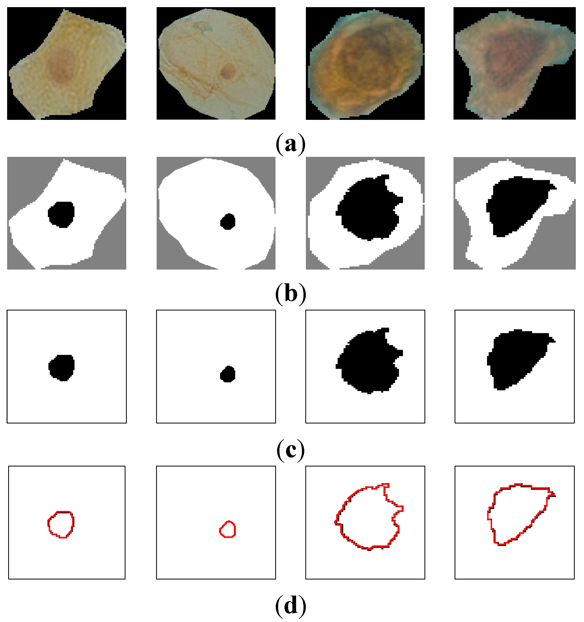
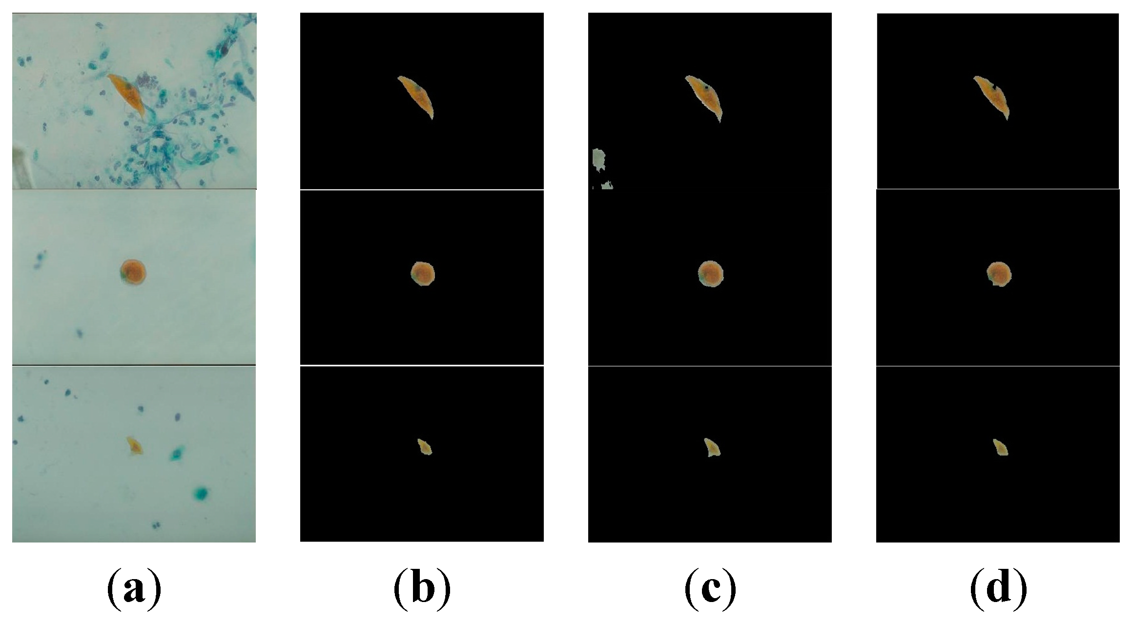
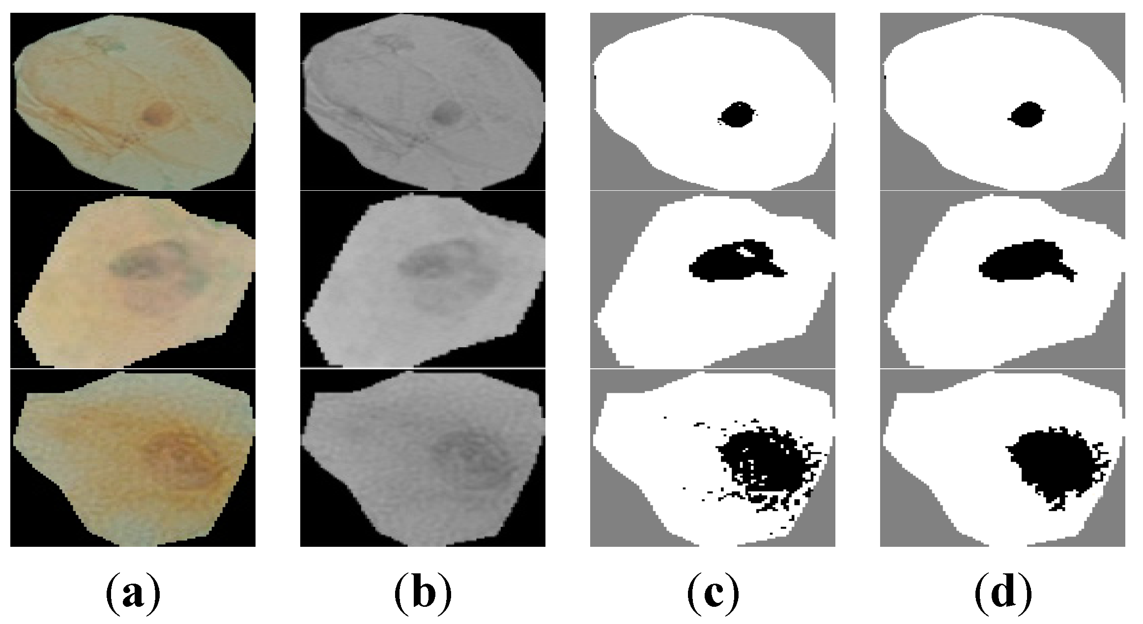
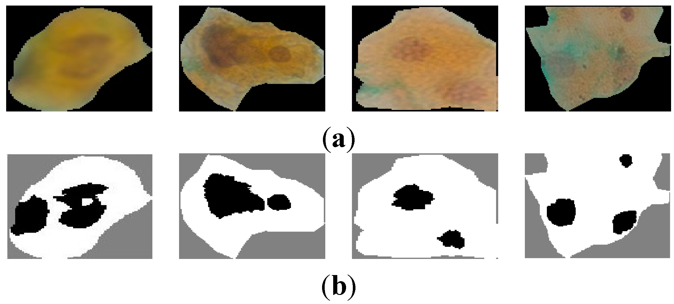
Figure 5a shows samples of extracted nuclei and cytoplasm.
Figure 5b depicts the nucleus and cytoplasm extraction where the black and white areas represent the nucleus and the cytoplasm respectively.
Figure 5c shows the nucleus area.
The second feature is the nucleus perimeter defined by:
where
x(
t) and
y(
t) are the parameterized contour point coordinates. In the discrete case,
x(
t) and
y(
t) are defined by a set of pixels in the image. Thus, Equation (4) is approximated by:
Figure 5d depicts the perimeter area in color red for the nuclei cell in
Figure 5c.
Figure 5.
(a) raw sputum cells; (b) nucleus and cytoplasm segmentation; (c) nucleus region; (d) the perimeter of the nucleus area.
Figure 5.
(a) raw sputum cells; (b) nucleus and cytoplasm segmentation; (c) nucleus region; (d) the perimeter of the nucleus area.
The third feature representing the density is based on the darkness of the nucleus area after staining with a certain dye, thus it is based on the mean value of the nucleus region. The mean value represents the average intensity value of all pixels that belong to the same region, and in our case, each mean value is represented as a vector of RGB components, and is calculated as follows for a given nucleus:
where
i is the intensity color value and
N is the total number of the pixels in the nucleus area.
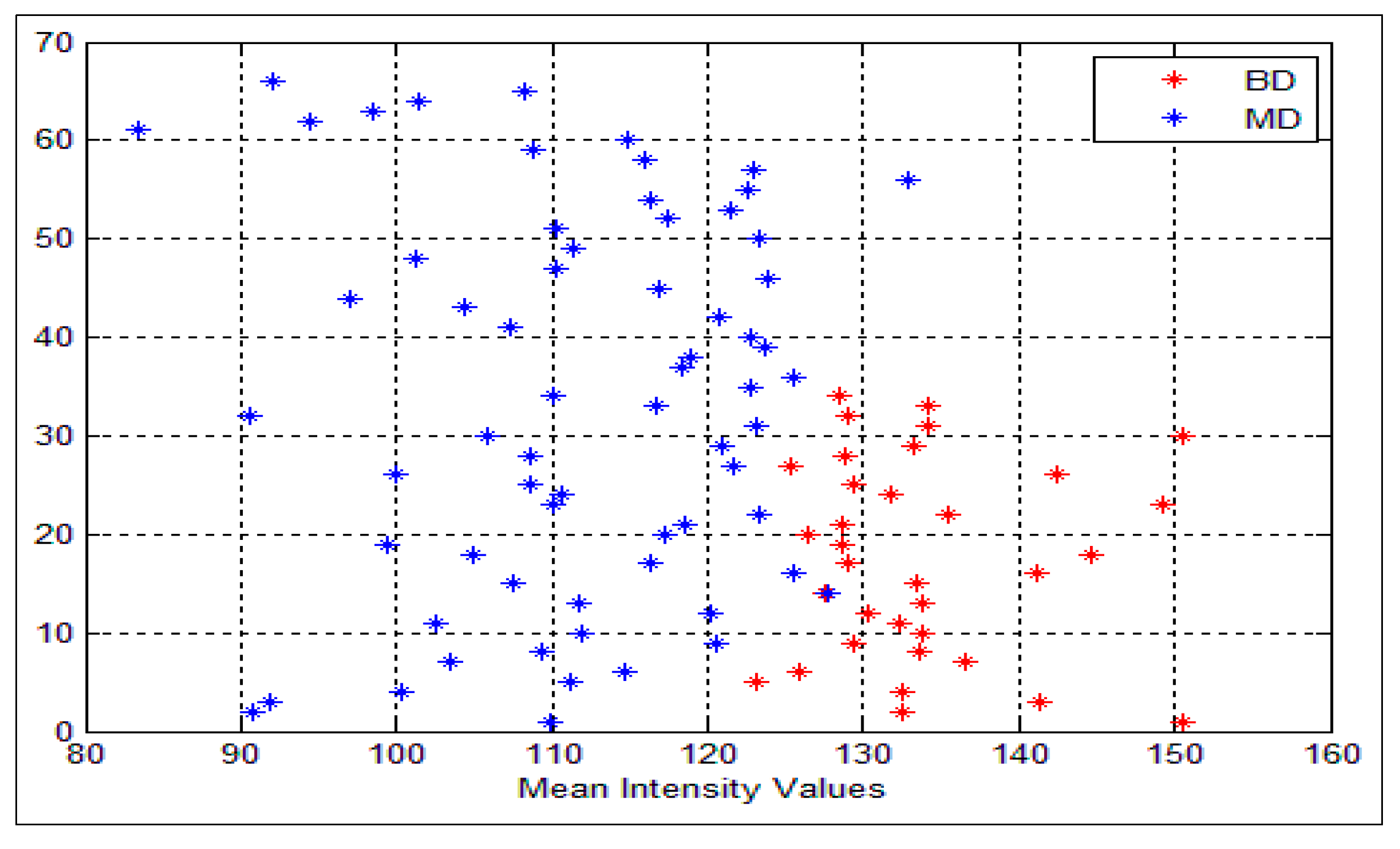
Figure 6 shows the mean intensity values for both benign and malignant cells. As can be seen, all the values that are greater than or equal to the threshold value θ are classified as benign cells (color red) and, the other values which are less than θ are classified as malignant (color blue), BD and MD refer to the benign and malignant density respectively. In our system θ = 128. Nevertheless, some overlapping does exist, where very few malignant cells are classified as benign cells (FN) and vice versa. In this situation, we cannot consider the intensity feature alone.
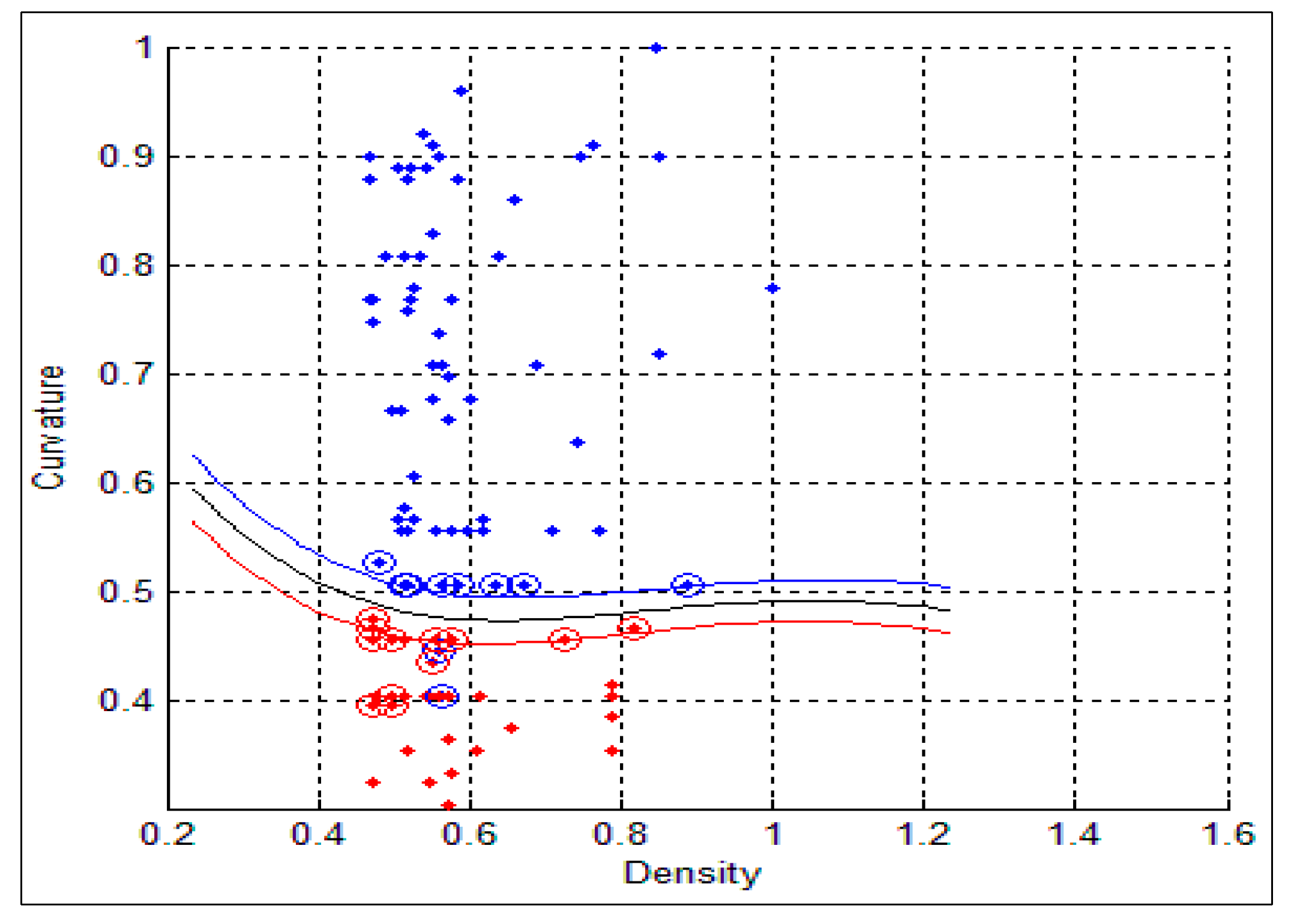
The fourth feature is the curvature, which is delineated by the rate of change in the edge direction. This rate of change characterizes the points in a curve which are known as corners where the edge direction changes rapidly [
18]. A lot of significant information can be extracted from these points. The curvature at a single point in the boundary can be defined by its adjacent tangent line segments. The difference between slopes of two adjacent straight line segments is a good measure of the curvature at that point of intersection [
19]. The slope is defined by:
where
and
denote the derivative of
x(
t) and
y(
t). We computed the difference between adjacent slopes (δθ) for each point in the nucleus contour.
Figure 6.
Intensity variances for the nuclei cells, the blue represents the malignant cells (MD) and the red represents the benign cells (BD).
Figure 6.
Intensity variances for the nuclei cells, the blue represents the malignant cells (MD) and the red represents the benign cells (BD).
In our data, we found that in the case of malignant cells, δθ goes above a threshold estimated to 50.
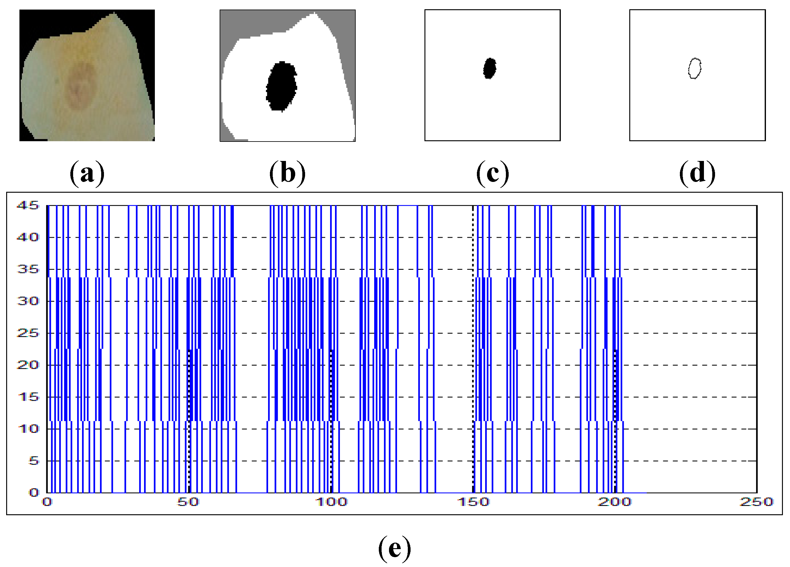
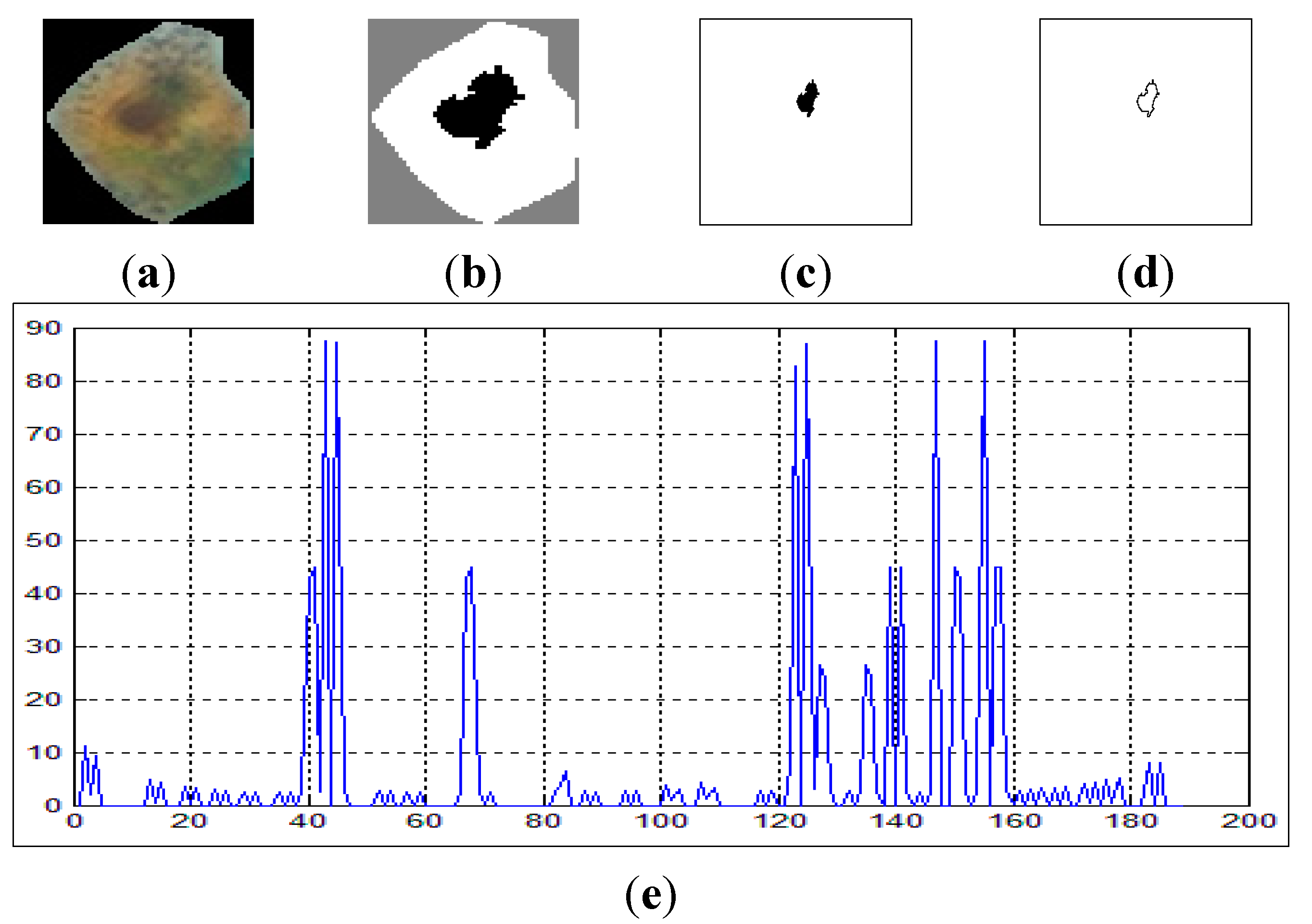
Figure 7 shows the curvature extraction (δθ) of the benign cell.
Figure 7a shows the benign sputum cell and
Figure 7d shows the boundary, which is used to compute the curvature.
Figure 7e depicts the curvature where the
x-axis represents the slope between the points in the image boundaries and the
y-axis represents the curvature. As can be seen from this figure, all the lines are between 0° and 45°, and no line exceeds our δθ = 50.
Figure 7.
The curvature extraction of a benign cell. (a) Sputum cell; (b) Nucleus and cytoplasm segmentation; (c) Nucleus extraction; (d) Nucleus boundary and (e) reflects the curvature plot for the image boundary in (d).
Figure 7.
The curvature extraction of a benign cell. (a) Sputum cell; (b) Nucleus and cytoplasm segmentation; (c) Nucleus extraction; (d) Nucleus boundary and (e) reflects the curvature plot for the image boundary in (d).
On the other hand,
Figure 8 shows the curvature extraction of a malignant cell. As can be seen from
Figure 8e, there are some lines in the curvature (
y-axis) which exceed δθ = 50, and this is a clear reflection of the irregularities in the boundary of the cell.
Figure 8.
The curvature extraction of a malignant cell. (a) sputum cell; (b) nucleus and cytoplasm segmentation; (c) nucleus extraction; (d) nucleus boundary and (e) reflects the curvature plot for the image in (d).
Figure 8.
The curvature extraction of a malignant cell. (a) sputum cell; (b) nucleus and cytoplasm segmentation; (c) nucleus extraction; (d) nucleus boundary and (e) reflects the curvature plot for the image in (d).
The fifth feature is the circularity, which is a feature that describes the roundness of the nucleus, and is defined as
Cells in cleavage are normally round, so their roundness value will be higher. On the other hand, normal growing cells are irregular so their roundness value will be lower. For the circularity, it should be less than or equal to 1 within the threshold ratio, to distinguish between normal and abnormal cells, where 1 means a perfect circle [
20].
The last feature is the Eigen ratio [
21]. In our system, irregular cells are long, thus expected to have a higher Eigen ratio than that of round floating cells. Thus, using a proper threshold value we can distinguish between benign and malignant cells with this feature. The Eigen ratio is computed as follows:
where (
a,
b) are the eigenvalues of the covariance matrix
C, defined by:
where
is a point in the nucleus area. The eigenvalues (
a,
b) are used to show the direction of the cell distribution in the nucleus region in the horizontal direction by using value of (
a) and in the vertical direction by using value of (
b).
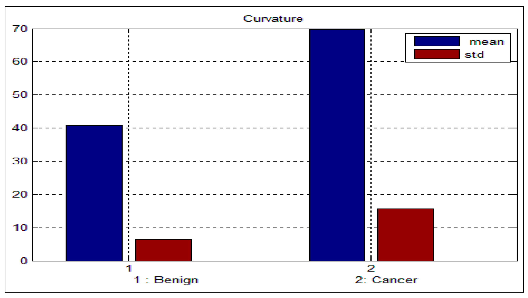
Table 3 and
Table 4 depict the mean and standard deviation (
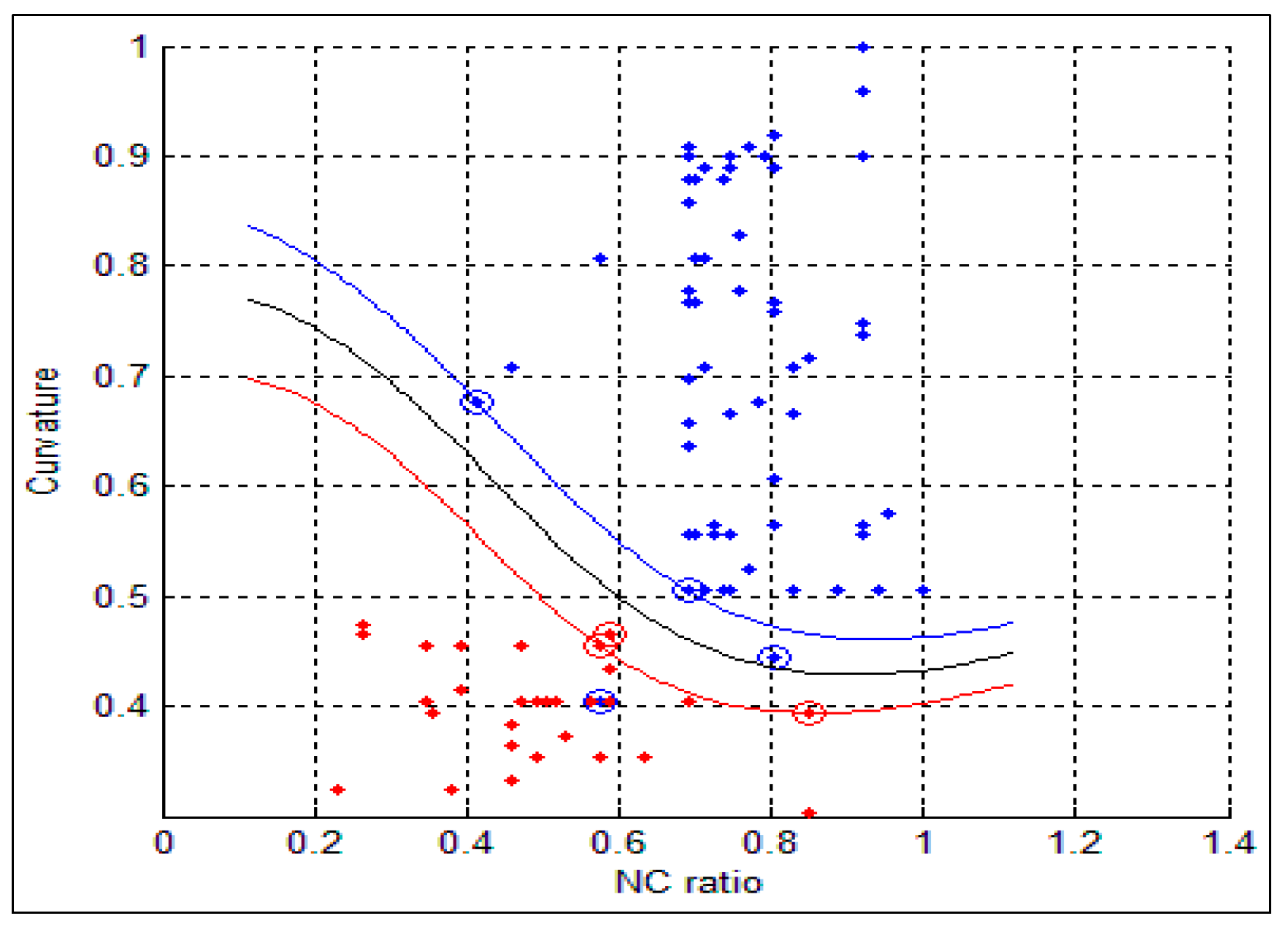
std) for the benign and malignant cells, respectively. As can be seen from these two tables, there is a big difference between the mean and std for benign and malignant cells, thus indicating the potential of the proposed features for discriminating between benign and malignant cells. In addition to this, the NC ratio and the curvature show the possibility of linear separation between the benign and malignant cells.
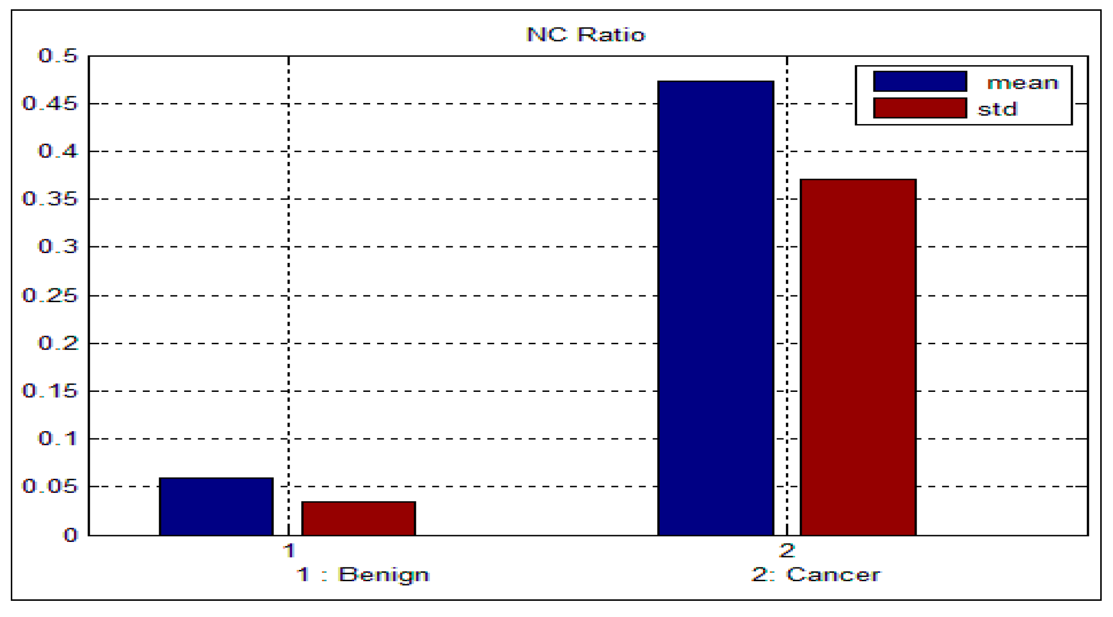
Figure 9 and
Figure 10 show the bar chart of the mean and standard deviation for the malignant and benign cells for the NC ratio and curvature.
Table 3.
Mean and standard deviation for the benign sputum cell.
Table 3.
Mean and standard deviation for the benign sputum cell.
| Features | NCratio | Perimeter | Density | Curvature | Circularity | Eigen Rati |
|---|
| Mean | 0.06 | 87.8 | 128.3 | 40.88 | 0.44 | 1.21 |
| Std | 0.03 | 27.9 | 9.5 | 6.46 | 0.12 | 0.22 |
Table 4.
Mean and standard deviation for the malignant sputum cell.
Table 4.
Mean and standard deviation for the malignant sputum cell.
| Ftures | NCratio | Perimeter | Density | Curvature | Circularity | Eigen Rati |
|---|
| Mean | 0.47 | 124.3 | 113.4 | 69.59 | 0.55 | 1.42 |
| Std | 0.37 | 41.1 | 12.1 | 15.57 | 0.16 | 0.22 |
Figure 9.
Mean and standard deviation for the NC ratio.
Figure 9.
Mean and standard deviation for the NC ratio.
Figure 10.
Mean and standard deviation for the curvature.
Figure 10.
Mean and standard deviation for the curvature.
7. Conclusions
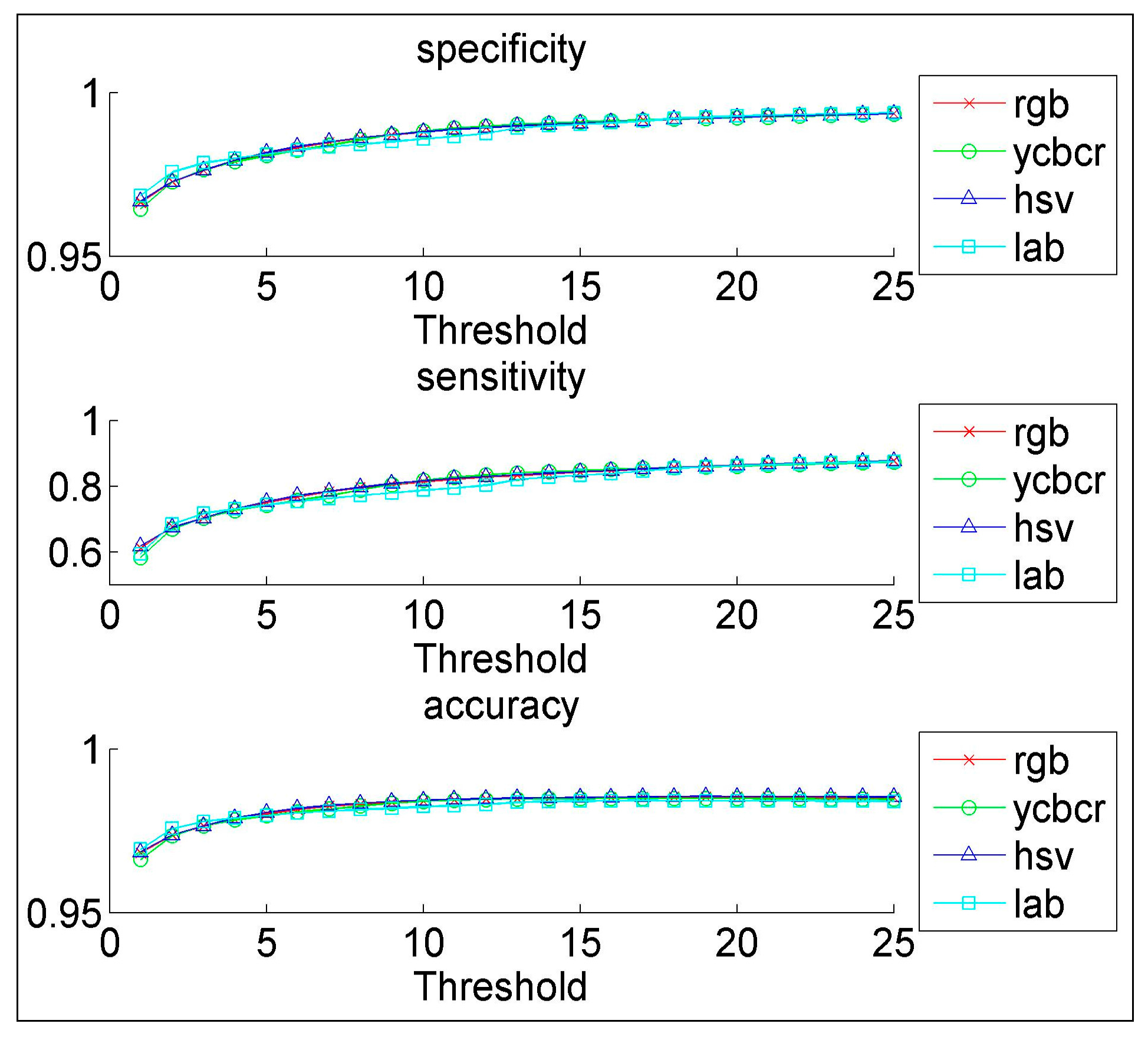
We have proposed a novel CAD system for the early diagnosis of lung cancer. We have used a database of 100 sputum color images for different patients collected by the Tokyo center of lung cancer. The new CAD system can process sputum images and classify them into benign or malignant cells. For the color quantization, it was found that, the higher the color space resolution, the more accurate the detection and extraction of the sputum cell. It was found that the Bayesian classification is better than the heuristic rule-based classification as the former achieved an accuracy of 98%. The comparability of the performance with regard to the color format reveals close scores for histogram resolution above 64. In the segmentation process, it was demonstrated that the mean shift approach significantly outperforms the HNN technique, especially after acquiring additional information such as pixel space coordinates. The mean shift has a reasonable accuracy of 87%.
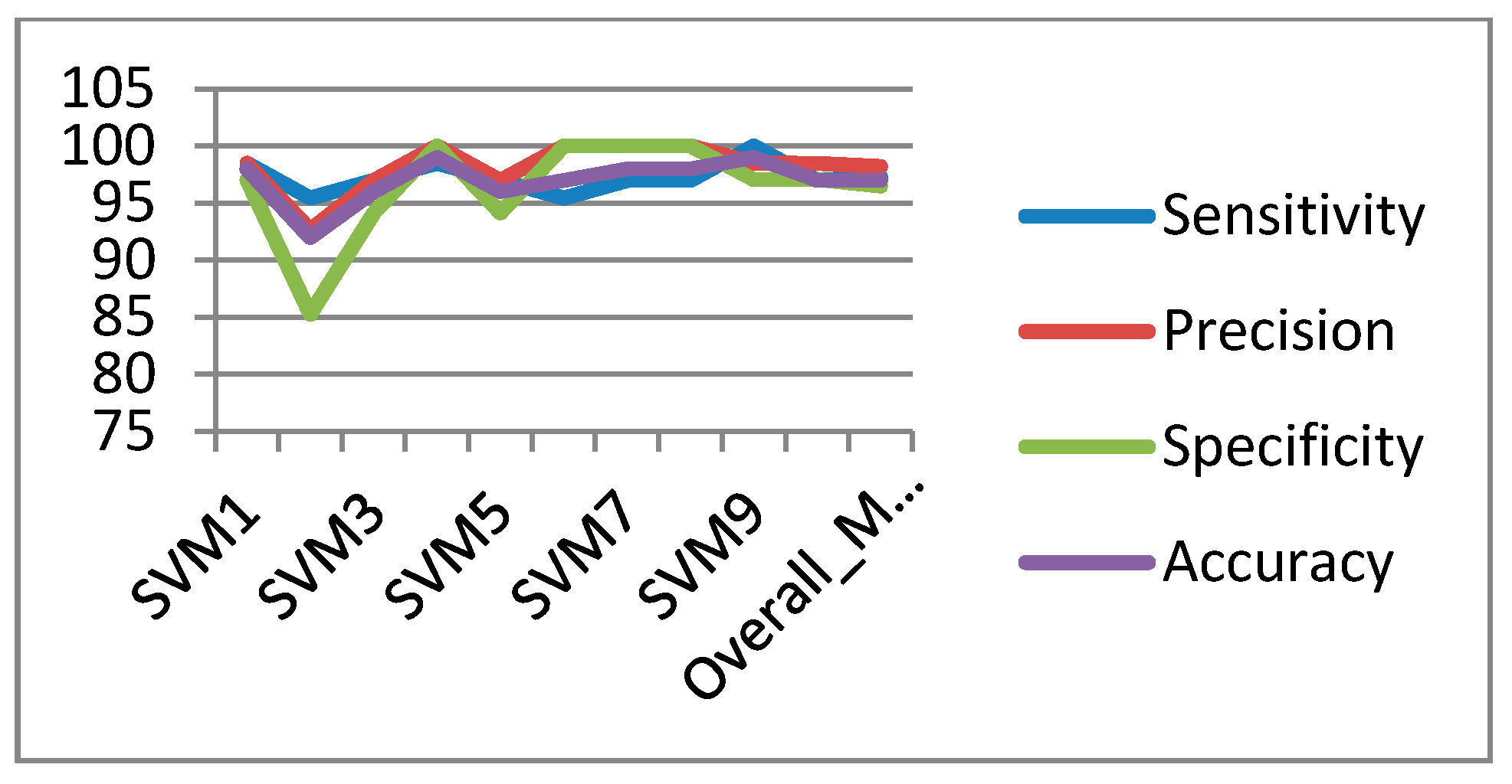
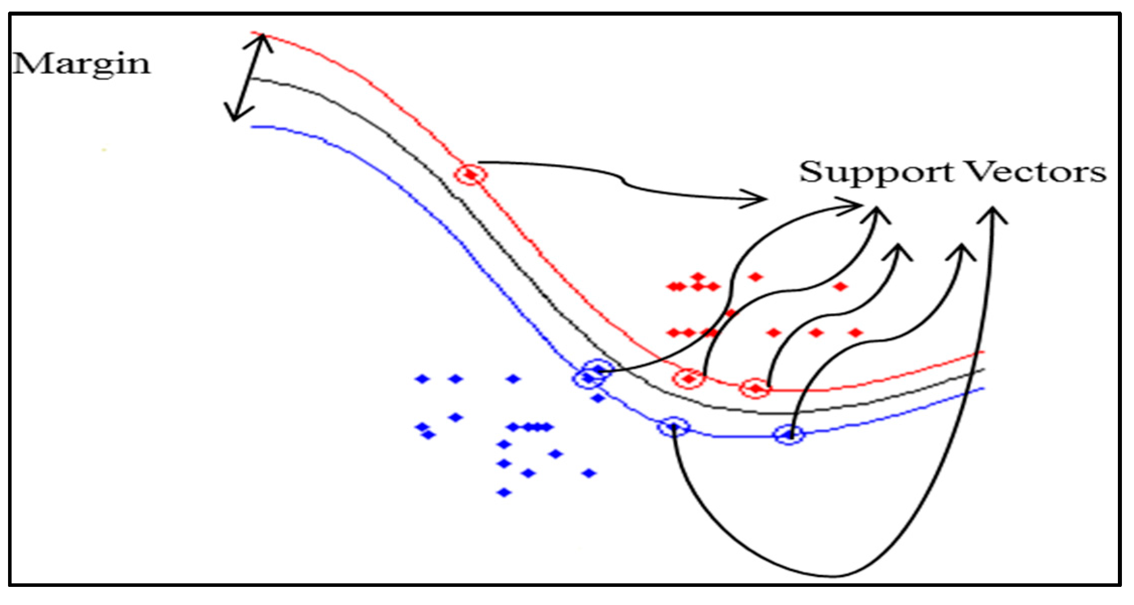
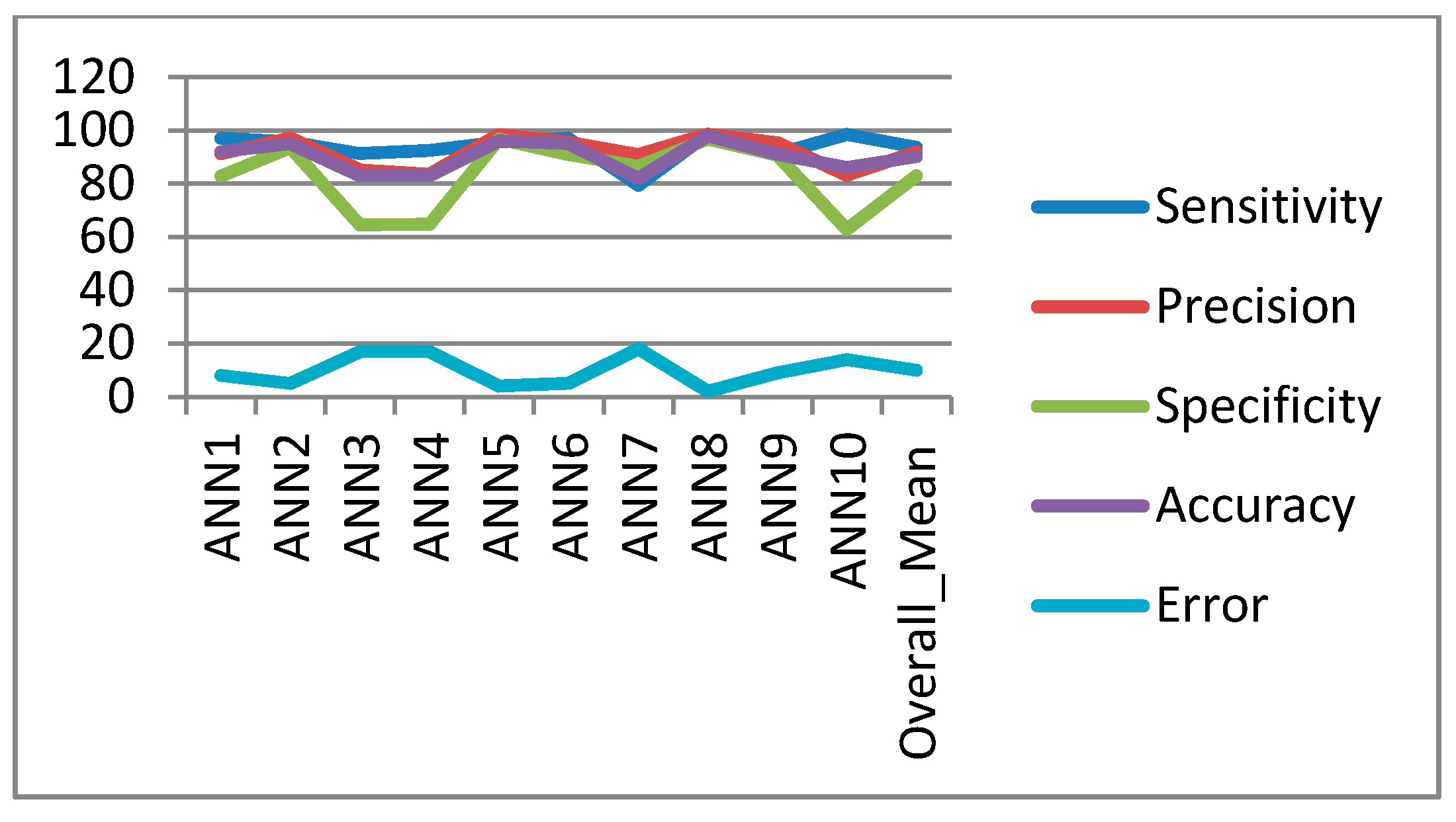
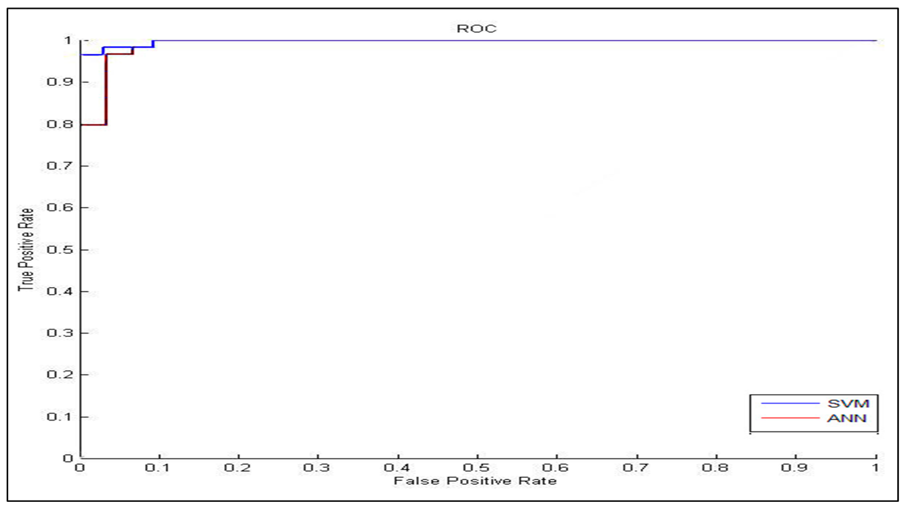
In the classification process: it was found that the performance of the SVM is superior compared to the ANN classifier. The SVM classifier allows a clear separation and classification of the cells into benign and malignant classes. Therefore, it is more stable and reliable for the proposed CAD system. The SVM achieved an accuracy of 97%. The experimental result shows that the proposed CAD system is able to detect the false positives and false negatives correctly. The new system has achieved a good performance in terms of sensitivity, specificity and accuracy equal to: 97%, 96% and 97% respectively. In addition, the use of extreme SVM as a learning model increased the accuracy of detecting the malignant cells. The new CAD system will be useful in screening a large number of people for lung cancer while helping pathologists to focus on candidate samples, and reducing the pathologists fatigue to a great extent.
With respect to the experimental work described in this paper, there is also considerable further work which could be undertaken. To solve the problem of inhomogeneity in the cytoplasmic region, we plan to use active contour snake segmentation which has the ability to work with images that have an overlapped nucleus and cytoplasm. This will be done by using Otsu’s automated thresholding selection method to segment the dysplastic sputum cells due to high inhomogeneities between the cells. We plan to extend the research to address these limitations as well as use a more extended data set of available sputum images.


