All articles published by MDPI are made immediately available worldwide under an open access license. No special
permission is required to reuse all or part of the article published by MDPI, including figures and tables. For
articles published under an open access Creative Common CC BY license, any part of the article may be reused without
permission provided that the original article is clearly cited. For more information, please refer to
https://0-www-mdpi-com.brum.beds.ac.uk/openaccess.
Feature papers represent the most advanced research with significant potential for high impact in the field. A Feature
Paper should be a substantial original Article that involves several techniques or approaches, provides an outlook for
future research directions and describes possible research applications.
Feature papers are submitted upon individual invitation or recommendation by the scientific editors and must receive
positive feedback from the reviewers.
Editor’s Choice articles are based on recommendations by the scientific editors of MDPI journals from around the world.
Editors select a small number of articles recently published in the journal that they believe will be particularly
interesting to readers, or important in the respective research area. The aim is to provide a snapshot of some of the
most exciting work published in the various research areas of the journal.
Kung-Traub conjecture states that an iterative method without memory for finding the simple zero of a scalar equation could achieve convergence order , and d is the total number of function evaluations. In an article “Babajee, D.K.R. On the Kung-Traub Conjecture for Iterative Methods for Solving Quadratic Equations, Algorithms 2016, 9, 1, doi:10.3390/a9010001”, the author has shown that Kung-Traub conjecture is not valid for the quadratic equation and proposed an iterative method for the scalar and vector quadratic equations. In this comment, we have shown that we first reported the aforementioned iterative method.
1. Iterative Methods for Solving Quadratic Equations Presented in [1]
According to Kung-Traub conjecture (KTC) [2], an iterative method without memory for solving nonlinear equations in the case of simple zeros, could achieve a maximum convergence order of , where d is the number of function evaluations. Recently, an article was published for solving quadratic equations [1] with arbitrary order of convergence by using one function and two derivatives evaluations. The details of the proposed formulation in [1] is given as follows. Let be a quadratic function where and , are constants. The proposed iteration function in [1] is
The error equation of Equation (1) is given as where is asymptotic error constant, is the simple root of quadratic equation and . The error equation clearly shows that KTC is not valid in the case of quadratic equations. By using binomial expansion, the weight function can be written as
where is constant and can be computed by comparing two expressions of in Equation (2). The powers of τ can be computed recursively and hence the iteration function Equation (1) is written as
The computationally efficient vector version of iteration function Equation (3) is
2. Iterative Methods for Solving Matrix-Vector Quadratic Equations Presented in [3]
In this direction, a manuscript [3] was posted on 4 May 2015 on Researchgate in which the author provided models of three iterative methods, with their respective convergence orders, for computing the solution of matrix-vector quadratic equations. As the proposed iterative methods are valid for solving systems of nonlinear equations with quadratic nonlinearity, they are also valid for scalar quadratic equations. In the article [3] the model of iterative Method II can be written as:
where is a quadratic equation i.e., is a bilinear form and (zero tensor) for and the convergence order is . The scalar version of iterative method Equation (5) can be written as
where with and convergence order is . The convergence proofs of different iterative methods are established in Figure 1, Figure 2, Figure 3 and Figure 4. We can see that the error equations in all cases are the same. The Figure 4 shows that the iterative method (1) is a particular case of iterative method Equation (6) for . Finally we provide the convergence proof of the iterative method Equation (5).
Theorem 2.1.
Letbe a function with all continuous Fréchet derivatives,andfor , whereis a bilinear form andis convex open subset of . If we takein the vicinity of a simple rootofthen the sequence of successive approximation generated by iterative method Equation (5) forandconverges towith convergence order eight.
Proof.
We denote , and . By expanding around we get
The Fréchet derivative of Equation (7) with respective to is
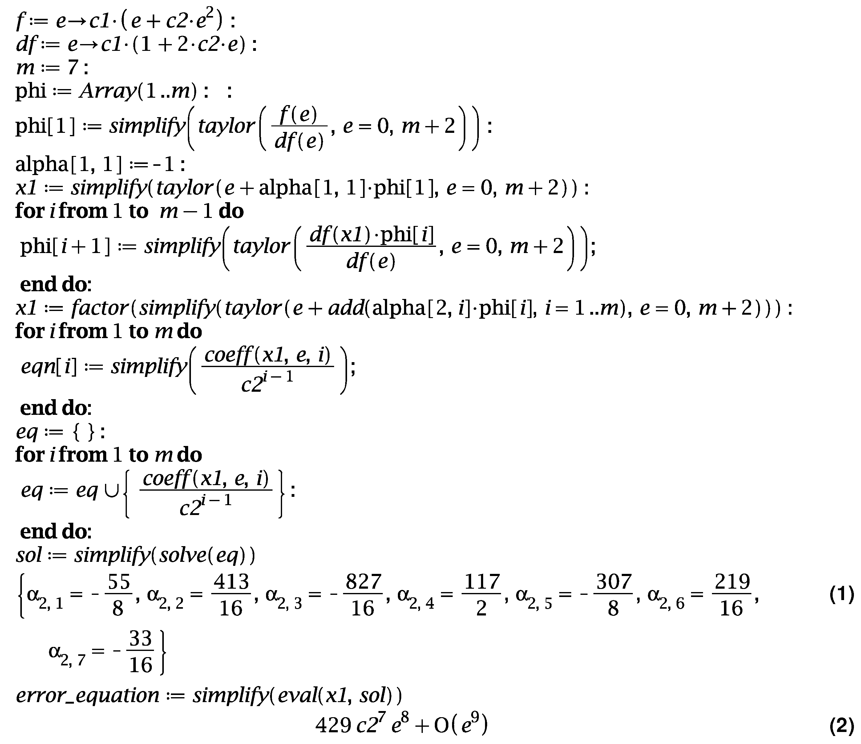
By equating the coefficients of powers of in Equation (15), we get system of seven equations
The solution set of seven equations is
After simplification the error equation we get
☐
As we have seen, the convergence order of the iterative method Equation (5) is eight for and this confirms our claimed order of convergence which is for . Now we provide the proof of convergence order via mathematical induction.
Theorem 2.2.
Letbe a function with all continuous Fréchet derivatives,andfor , whereis a bilinear form andis a convex open subset of . If we takein the vicinity of a simple rootofthen the sequence of successive approximation generated by the iterative method Equation (5) forandconverges towith convergence order .
Proof.
We suppose that our claim about the convergence order of the iterative method Equation (5) is true for , which means we have
where is asymptotic error constant and superscript “” means the value of when . We can write
It is convenient to express the combination
in the powers of [1], we establish the following identity
By comparing the same powers of on both sides we can easily compute the value of ’s. By using Equation (21), error Equation (20) can be written as
However, according to our assumption we can find the value of unknowns to make the following expression equal to zero
As we know the value of we can find to make the coefficient of equals to zero. Hence we get
which completes the proof. ☐
3. Numerical Testing
We adopt the following definition of computational convergence order (COC)
To verify the claimed convergence order of our proposed iterative method Equation (5), we study the following system of quadratic equations
In Table 1, we listed the norm of the residue of and COC against the sequence of iterations for different values of parameters . The Table 1 confirms the claimed convergence order. For two different values of the parameter , we obtained the record of the norm of the residue of equal to the system of quadratic Equations (26). The possible reason for his could be the same error equation of iterative method for different values of parameter in the iterative method Equation (5).
4. Conclusions
We conclude that the iterative structure of iterative method Equation (1) was first reported in article [3] as a particular case and our proposed iterative method [3] is general because is a free parameter.
Conflicts of Interest
The author declares no conflict of interest.
References
Babajee, D.K.R. On the Kung-Traub Conjecture for Iterative Methods for Solving Quadratic Equations. Algorithms2016, 9, 1. [Google Scholar] [CrossRef]
Traub, J.F. Iterative Methods for the Solution of Equations; Prentice-Hall: Englewood Cliffs, NJ, USA, 1964. [Google Scholar]
Ahmad, F. Higher Order Iterative Methods for Solving Matrix Vector Equations. Researchgate2015. [Google Scholar] [CrossRef]
Ahmad, F.
Comment on: On the Kung-Traub Conjecture for Iterative Methods for Solving Quadratic Equations. Algorithms 2016, 9, 1. Algorithms2016, 9, 30.
https://0-doi-org.brum.beds.ac.uk/10.3390/a9020030
AMA Style
Ahmad F.
Comment on: On the Kung-Traub Conjecture for Iterative Methods for Solving Quadratic Equations. Algorithms 2016, 9, 1. Algorithms. 2016; 9(2):30.
https://0-doi-org.brum.beds.ac.uk/10.3390/a9020030
Chicago/Turabian Style
Ahmad, Fayyaz.
2016. "Comment on: On the Kung-Traub Conjecture for Iterative Methods for Solving Quadratic Equations. Algorithms 2016, 9, 1" Algorithms 9, no. 2: 30.
https://0-doi-org.brum.beds.ac.uk/10.3390/a9020030
Note that from the first issue of 2016, this journal uses article numbers instead of page numbers. See further details here.
Article Metrics
No
No
Article Access Statistics
For more information on the journal statistics, click here.
Multiple requests from the same IP address are counted as one view.
Ahmad, F.
Comment on: On the Kung-Traub Conjecture for Iterative Methods for Solving Quadratic Equations. Algorithms 2016, 9, 1. Algorithms2016, 9, 30.
https://0-doi-org.brum.beds.ac.uk/10.3390/a9020030
AMA Style
Ahmad F.
Comment on: On the Kung-Traub Conjecture for Iterative Methods for Solving Quadratic Equations. Algorithms 2016, 9, 1. Algorithms. 2016; 9(2):30.
https://0-doi-org.brum.beds.ac.uk/10.3390/a9020030
Chicago/Turabian Style
Ahmad, Fayyaz.
2016. "Comment on: On the Kung-Traub Conjecture for Iterative Methods for Solving Quadratic Equations. Algorithms 2016, 9, 1" Algorithms 9, no. 2: 30.
https://0-doi-org.brum.beds.ac.uk/10.3390/a9020030
Note that from the first issue of 2016, this journal uses article numbers instead of page numbers. See further details here.


