Introducing the Green Infrastructure for Roadside Air Quality (GI4RAQ) Platform: Estimating Site-Specific Changes in the Dispersion of Vehicular Pollution Close to Source

Abstract

The benefits of ‘green infrastructure’ are multi-faceted and well-documented, but estimating those of individual street-scale planting schemes at planning can be challenging. This is crucial to avoid undervaluing proposed schemes in cost–benefit analyses, and ensure they are resilient to ‘value engineering’ between planning and implementation. Here, we introduce prototype software enabling urban practitioners to estimate the site-specific air quality impacts of roadside vegetation barriers: highly localised changes in pollutant concentrations due to changes in the dispersion of vehicular emissions close to source. We summarise the recent shift in understanding regarding the impacts of vegetation on urban air pollution towards changes in pollutant dispersion (cf. deposition) and describe our prototype software, offering rapid estimates thereof. First tests of the underlying model’s performance are promising, reproducing: annual mean NO₂ and PM_2.5 concentrations in a street canyon (Marylebone Road, London, UK) to within 10% and 25%, respectively; and changes in pollutant concentrations of the right order of magnitude behind roadside barriers in a wind tunnel simulation of a street canyon and a real open-road environment. However, the model underestimates the benefits of a barrier in a simulated street canyon under perpendicular wind conditions. The prototype software is a first step towards informing practitioners of the site-specific impacts of vegetation barriers, which should always be additional to (i.e., no substitute for) essential emission reductions. The code is open-source to engage further researchers in its continued development.

1. Introduction

Urban forests and ‘green infrastructure’ bring many benefits to our towns and cities, including increased biodiversity, sustainable urban drainage, mitigation of the urban heat island effect and improved air quality (see, e.g., [1,2,3,4]). We tend to categorise these benefits as environmental in kind, but, directly or indirectly, many of them translate to economic benefits via cost savings, such as reduced mains drainage costs (see, e.g., [5]), reduced indoor cooling costs (see, e.g., [6]) and reduced health damage costs linked to air pollution (see, e.g., [7,8]). For example, the London i-Tree Eco Project estimated that the UK capital’s 8.4 million trees, collectively, deliver benefits of over £130 million per year [9]. A similar study, commissioned by Toronto Urban Forestry, estimated that the 10.2 million trees in Canada’s largest city provide ecological services worth $60 million per year [10]. Recognition of the benefits, or ‘nature based solutions’ [11], delivered by this natural capital can support the preservation of existing green infrastructure (e.g., justifying maintenance costs) and investment in further green infrastructure. It can be a challenge, however, for non-specialists to quantify at planning (including, but not limited to, the official process of obtaining planning permission) the environmental benefits, let alone the economic value, of an individual street planting scheme. Quantitative estimation of benefits at planning is essential to enhance a scheme’s resilience to cost-cutting between design and implementation. Our understanding of urban green infrastructure has evolved rapidly in recent years, particularly regarding exposure to urban air pollution. Here, we introduce prototype software enabling urban practitioners to estimate the site-specific air quality impacts of street planting at planning.

This paper has two specific aims: (1) to introduce the prototype Green Infrastructure for Roadside Air Quality, or ‘GI4RAQ’, Platform; and (2) to present the first tests of its performance (comparisons with real-world measurements and wind tunnel studies). We describe the model concept, logic, and code in some detail, drawing particular attention to features that differentiate it from existing tools (e.g., Gaussian dispersion models and the i-Tree tool; www.itreetools.org, accessed on 4 June 2021). The prototype Platform’s air quality code should be regarded simply as a framework, which conserves mass but is currently based on some crude assumptions and approximations; this framework will, however, readily accept parameters generated with the aid of more sophisticated models. We describe the limitations of the current release, and point to further developments that would increase its predictive skill and scope without adding undue complexity.

The software is applicable to the design of streets in new developments, where it can aid the side-by-side planning of grey and green infrastructure, but also to the redesign of existing streets as part of grey infrastructure modification to encourage modal shift and incorporate planting for reduced pedestrian and cyclist exposure. Initiatives to increase provisions for active travel (e.g., Transport for London’s Cycleways [12] and Transport for Manchester’s ‘Beelines’ [13]) may offer opportunities to incorporate planting to reduce cyclist and pedestrian exposure to vehicular pollution. Such initiatives have gained momentum as social-distancing, in response to COVID-19, has demanded a rebalancing of spatial allocations in streets between motorised transport and active travel (e.g., Streetspace Plan for London [14]). When used in street redesign, GI4RAQ will be used alongside many other design checks and balances to consider, for example, traffic safety, visibility, biodiversity and maintenance issues.

1.1. Exposure to Air Pollution at the Roadside

Road transport is the largest single source of urban outdoor air pollution (see, for example, the review of studies identifying and apportioning the sources of particulate matter (PM), spanning 51 countries [15]). Whilst the exhaust component of road transport pollution will decline with the move to electric (and hydrogen-fuelled) vehicles, electrification will not reduce and could even exacerbate its non-exhaust components: brake, tyre and road wear [16,17,18]. At points of friction between brakes and wheels, or wheels and roads, vehicles generate PM, and electric vehicles laden with heavy batteries may generate more PM due to their greater weight [18].

The best way to improve air quality is to reduce emissions at source (e.g., via modal shift to public transport and active travel), but reducing exposure to these emissions offers a means of further reducing their health impacts. The concentrations of pollutants are highest where they are emitted, rapidly decaying towards their urban-average ‘background’ concentrations with increasing distance from source. The roadside environment, in which large numbers of people come into close proximity with vehicles, is therefore a priority area for exposure reduction. It is also an environment where vegetation barriers, in the right locations, have potential to reduce local exposure; we refer to recent reviews [19,20,21].

Vegetation at the scale of realistic urban planting schemes has only a minor influence on local air quality via its emissions of volatile organic compounds (see, e.g., [22] and references therein), which can be mitigated via careful species selection (see, e.g., “Urban Tree Air Quality Score” [23]). It also typically removes only a few percent of PM and an even smaller fraction of nitrogen dioxide (NO₂) and, yet, vegetation barriers can reduce exposure to proximate sources of pollution by as much as 50% in their immediate wake [20,24]. That is, barriers can change the distribution of pollution close to source by altering the flow of polluted air and, hence, its mixing with cleaner surrounding air. Changing the local distribution of pollution implies a mixture of benefits and disbenefits in the vicinity of a vegetation barrier, the sizes and locations of which will be complex functions of site-specific conditions.

This complexity could underpin the wide range of findings relayed in [19]’s relatively early review of ‘air pollution abatement performances of green infrastructure’. Not only do different studies cited therein report different impacts (ranging, approximately, from a 70% reduction, to a 250% increase, in pollutant concentrations; see their Figure 3), but some studies individually report a wide range of effects. For instance, [25]’s computational fluid dynamics (CFD) study of the impacts of tree canopies in a narrow street reported concentration increases at the equivalent of head height of between 0 and 120%; their Figure 10 illustrates dependencies on both the configuration of trees within the street, and the wind direction relative to the street.

The most recent review of ‘urban vegetation in air quality management’ [21] concluded that studies to date do not support generalised guidance on the design of suitable interventions, as each study’s findings are limited to site-specific meteorological or morphological conditions. Authors in [21] also noted, with reference to [26,27], that our knowledge of the impact of urban form on the flow of air and pollution dispersion is not yet adequately applied in urban planning and decision making. The prototype GI4RAQ Platform utilises this knowledge to estimate the site-specific impacts of proposed green (or grey) infrastructure barriers in specific locations, subject to local conditions of wind and urban form.

1.2. Deposition of Pollution to Street-Scale Vegetation

Numerous studies of the impacts of vegetation on urban air quality have reported sizeable benefits in local air quality downwind of a hedge and/or line of trees, and referred to the deposition, removal or ‘filtering’ of pollutants (see the reviews of [19,28,29,30,31] and the primary studies cited therein). It is clear that deposition occurs, and is of benefit for air quality, but it is of limited benefit in most urban contexts unless the timescale for deposition is relatively long [32,33]. The benefits of deposition are dwarfed by the effects of urban vegetation on local pollution dispersion, be they positive or negative [20,24,34].

For instance, Macdonald et al. [35] and Donovan et al. [23] simulated the emission, transport and deposition of PM in the West Midlands (WM) and Glasgow, and explored the impacts of increased planting in each region. In the WM, they estimated that trees were responsible for removing 4% of primary PM₁₀, and the planting of a further 25% of land not already covered by hard surfaces (including important amenity areas, such as gardens and parkland) would reduce primary PM₁₀ concentrations by just 10%. In Glasgow, they estimated that the then-current removal of 3% of primary PM₁₀ could be bolstered to reduce PM₁₀ concentrations by just 2%, and even the planting of 100% of all areas not already covered by hard surfaces would yield only a 7% reduction. A more recent CFD model study [24] estimated that deposition to trees in central Leicester reduced PM_2.5 concentrations by 2.8%, but the effects of those trees on dispersion (not removing PM_2.5, but just altering its distribution) reduced PM_2.5 concentrations by 9%.

In a numerical model, it is relatively straightforward to separate the simulated effects of different mechanisms, such as deposition and dispersion. It is much more difficult, however, to differentiate between these based on measurements of pollutant concentrations before and after the introduction of a vegetation barrier (e.g., [36]). Attribution of concentration changes to the presence of a barrier requires prior elimination of the effects of all other factors that have changed between (and during) measurement periods, e.g., the strength of local emissions, background air pollutant concentrations and local wind conditions (e.g., [37,38]).

Measurements in controlled environments, such as wind tunnels, are appealing as they allow us to impose specific wind conditions. However, wind tunnel experiments, in which polluted air is forced through vegetation covering the tunnel’s entire cross-section (e.g., [39]), only tell us about the fraction of pollution removed from air passing through the vegetation. They tell us nothing about the air that, on encountering the physical obstruction posed by a vegetation barrier in a street, moves around it rather than through it.

1.3. Changing Pollution Dispersion Close to Source

Whilst deposition to vegetation, in the absence of its other effects, can only be beneficial (i.e., irrespective of where the vegetation is introduced), the impacts of vegetation on pollution dispersion may be of benefit or disbenefit to local air quality or, indeed, a combination of the two in different locations relative to it. The impacts of a vegetation barrier in ostensibly similar locations could also differ due to differences in: local wind conditions aloft; local urban form, with which those winds aloft interact; the strength of local emissions; the background air quality; and the precise positioning of vehicles, people, and the barrier introduced between the two. A strategic and selective approach is needed for planting in the name of improving local air quality. It is important to plant the right vegetation, in the right locations, to deliver genuine benefits where they are sought (i.e., ‘Right Tree, Right Place’ ethos [40]) and to avoid planting where it would be of disbenefit. The challenge is to predict the site-specific impacts of proposed barriers (i.e., the locations and magnitudes of accompanying benefits and disbenefits) and to enable urban practitioners to do so, irrespective of their specialist area of expertise, as part of comprehensive urban planning teams.

In the simplest scenario, where the wind blows consistently from vehicles towards people, and we introduce a vegetation barrier between the two, the concentrations of pollutants emitted by those vehicles can be expected to: increase immediately upwind of the barrier due to blocking; decrease in the immediate wake of the barrier, where a partially isolated region of overturning air is created by the fraction of polluted air diverted up and over the barrier; and relax towards the concentrations encountered before the barrier was introduced with increasing distance downwind [20].

Extensive literature, however, suggests that the wind direction at the base of a street is a complex function of interactions between the wind conditions aloft (i.e., above any buildings) and the local urban form. Harman et al. [41], for instance, synthesised the findings of multiple studies, from the 1980s [42] to the 2000s [43], in a formulation for street canyons of width (W) and height (H). When the wind aloft blows perpendicular to a street of W ≤ 3 H, it yields a reversal of air flow across the entire base of the street, relative to that aloft. Meanwhile, for a street of W > 3 H, it yields a reversal of air flow across just a fraction of its width (extending a distance of 3 H from its ‘upwind’ side; defined with respect to the wind direction aloft), whilst the direction of low-level air flow matches that aloft across the remainder of the street (see [41]’s Figures 1 and 2, and their accompanying text).

The local pattern of air flow could affect not only what is ‘upwind’ and what is ‘downwind’ of a barrier at the base of a street, but also the degree to which emissions are trapped within certain regions. The reversal of air flow at the base of a narrow street (W ≤ 3 H) is due to the creation of a vortex of overturning air in the wake of the buildings lining one side of that street, sometimes referred to as a ‘recirculation region’ [41], much the same as that created in the wake of a vegetation barrier. The partial isolation of air within a recirculation region could have profound consequences for local air quality, and the impacts of vegetation barriers. For instance, if vehicles lie within such a region, their emissions may be somewhat trapped and accumulate to higher concentrations. The addition of a vegetation barrier within the recirculation region would risk further reducing the volume of air in which the emissions are trapped, and further increasing their concentrations. Conversely, if all vehicles are excluded from such a region, it may represent an area of somewhat better air quality, partially isolated from proximate emissions; a vegetation barrier might be better employed between vehicles (outside this region) and people further downwind. We note that the patterns of air flow identified in CFD and wind tunnel simulations are not always observed in real streets (e.g., [44]), possibly due to the greater heterogeneity of real (cf. simulated) urban form and/or additional confounding factors, such as vehicle movements. Nonetheless, we expect the air flow within a street, and hence the impacts of a vegetation barrier on the dispersion of vehicular pollution close to source, to be a complex function of local conditions; there is no ‘one size fits all’ intervention.

1.4. Informing Urban Air Quality Interventions at Planning

Aligned with the scientific literature (as reviewed in [20]), and responding to urban planning needs (as identified in [21]), the prototype GI4RAQ Platform focuses exclusively on the impacts of vegetation on the dispersion of pollution close to source; it thereby complements the i-Tree tool (www.itreetools.org, accessed on 4 June 2021) that estimates only the benefits of pollutant deposition, accrued at much larger planting scales. Our prototype software offers estimates of the local air quality benefits and/or disbenefits of vegetation at street planting scales, where its benefits via enhanced deposition are expected to be dwarfed by the effects of that vegetation on the local dispersion, and hence distribution, of pollution [20]. In so doing, the software supports the consideration of public exposure at the level of individuals—perhaps particularly vulnerable individuals (i.e., the young, the old and those suffering from certain pre-existing medical conditions, such as chronic obstructive pulmonary disorder) and/or individuals in particularly polluted locations—to complement consideration of the total burden of air pollution (e.g., [7,8]).

In Section 2, we describe the air quality code underpinning the prototype software (2.1), referring the reader to Supplementary Materials for more technical details, and the model setups we have used to emulate real-world measurements and wind tunnel studies in the first tests of the code’s performance (2.2). We present the results to the performance tests in Section 3 and discuss their implications for the capabilities of the current prototype GI4RAQ Platform in Section 4. Here, we also outline the nature of future calibration-validation (cal/val) measurements, and the contributions the wider research community can make, by performing cal/val measurements or offering more sophisticated parameterisations to improve on the relatively simple relationships assumed in the current code. Although crude in places, the code is designed to capture the gross features of air flow and pollution dispersion as functions of local conditions and, coupled with the user interface (UI), enable a wide variety of urban practitioners to apply this mechanistic understanding to the design, or redesign, of streets from the earliest stages of planning.

2. Materials and Methods

2.1. Open Source Air Quality Code

The prototype GI4RAQ Platform (www.gi4raq.ac.uk, accessed on 4 June 2021) offers urban practitioners rapid, first-order estimates of the site-specific impacts of proposed barriers and, thereby, the ability to iterate on proposals in pursuit of their desired air quality outcomes (within the constraints of local conditions). This contrasts with most Gaussian dispersion models that do not inform practitioners of the potential impacts of within-street interventions. The user need only engage with a simple web-based UI, whilst the underlying air quality code handles the complexities outlined in Section 1. They are asked to ‘draw’ the cross-section of the street of interest to them, then specify the location of that street section (informing the wind conditions invoked aloft); its orientation (governing the interactions between the winds conditions aloft and the local urban form they have ‘drawn’, determining the pattern of air flow within the street); the locations and strengths of vehicular emissions of NO₂ and PM_2.5 within that street section; the background concentrations of NO₂ and PM_2.5, specific to that conurbation; and the nature of the barrier they propose introducing, including its dimensions, position, seasonality and ‘percentage obstruction’ when in leaf. These user-specified parameters are passed to our open-source air quality code (https://github.com/GI4RAQ/GI4RAQ-open, accessed on 4 June 2021) for analysis. This Python code determines the patterns of air flow and mixing within the street (i.e., treating NO₂ and PM_2.5 as passive tracers) with and without the proposed barrier, before passing the percentage differences in annual mean NO₂ and PM_2.5 concentrations back to the UI for display to the user; they are displayed in the form of two-dimensional pictures spanning the street section. Maintaining records of authorship (and user-specified parameters, on which the estimates are based), the user can then create PDF reports and invite others to iterate on their proposal.

The prototype GI4RAQ Platform is free to use, accessible to all and includes a comprehensive video User Guide. We have developed it in partnership with Wild Ilk Design Studio (www.wildilk.com, accessed on 4 June 2021) and a wide range of urban practitioners (see Acknowledgements). The remainder of Section 2.1, however, focuses on the underlying open-source air quality code, developed by the authors at the University of Birmingham specifically for the Platform. This code can be run ‘offline’ (i.e., independent of the UI), specifying the values of user-input parameters instead of drawing on those entered via the UI and passed to the code via a JSON string. Doing so offers greater flexibility. For instance, whilst the UI limits the software’s application to UK streets, due to the climatological wind data employed, the offline code is readily applicable to streets worldwide when coupled to suitable meteorological data.

The code comprises a two-dimensional model representative of the specified street section, in which steady-state concentrations are calculated in response to the other user-specified parameters, including emissions of NO₂ and PM_2.5 from specified ‘emission zones’; the flow of air into, around and out of the street section, described by ‘advection velocities’ at the interfaces between adjacent boxes, depending on the street’s geometry; and the mixing of air across these interfaces, described by ‘exchange velocities’. We refer to the (mean) flow of air as advection, and the turbulent mixing of air as dispersion. The mass-conservation model is outlined in Section 2.1.5 and elaborated on in Supplementary Materials Section S7; the crude means by which we currently estimate the advection and exchange velocities are described in Supplementary Materials Sections S5 and S6, respectively.

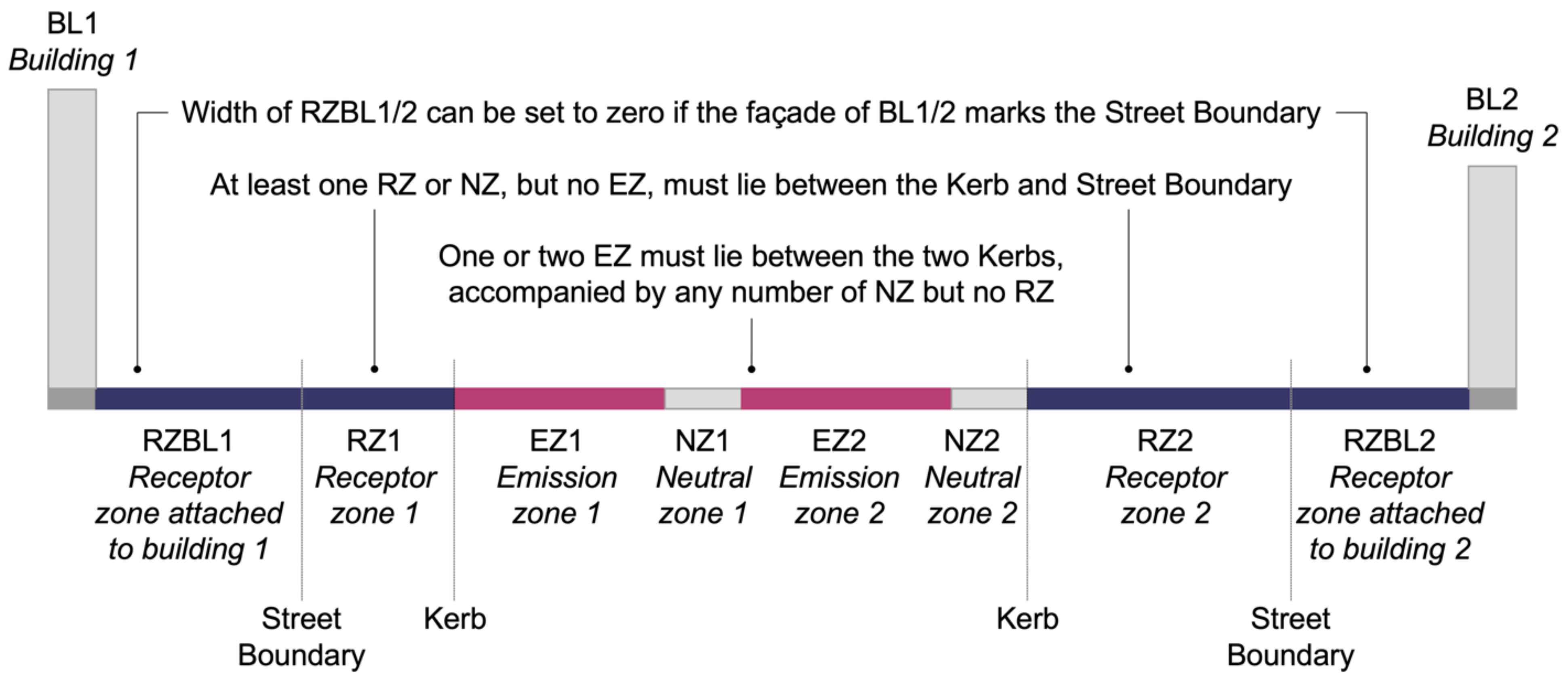
2.1.1. User-Specified Street Section

During the design process, we sought the most parsimonious description of a street cross-section that captured the most important (and most common) arrangements of emission source(s), green infrastructure, people and buildings. In the UI, the user is asked to dimension the cross-section of the street of interest to them: the heights of the nearest buildings on either side; and the distances by which their facades are set back from the respective ‘street boundaries’—i.e., the divisions between public and private realms. If a street is bounded by a large open space, such as a park, the distance to the nearest building on that side of the street (on a line perpendicular to the road) may be considered. That distance, however, is used to determine (in this case, rule out) the influence of that urban form on the flow of air in the vicinity of the road. The user is then asked to specify the distance between the two street boundaries, as they divide that space into a series of dimensioned zones, as illustrated in the example street section (Figure 1). The underlying model is applicable to streets of width-to-height ratio, W/H = 1 − ∞; it does not capture the creation of more than one vortex in particularly deep or narrow street canyons (W/H < 1).

The cross-section of a street bounded by Victorian terraced houses, for instance, may be quite uniform. In some streets, however, the urban form is much more heterogeneous. Here, we encourage users to explore the impacts of their proposed barrier subject to multiple street sections encountered in the street of interest to them, to test the sensitivity of the Platform’s estimates to its geometry (see Part 3 of the User Guide in the UI).

The street section is divided into three types of zone: receptor zones, emission zones and neutral zones. Receptor zones are spaces occupied by people, such as pedestrians and residents, generically referred to as ‘receptors’. Receptor zones are associated with no significant emissions, and could be a front garden between a building and a street boundary (e.g., RZBL1 in Figure 1) or a pavement between a street boundary and a kerb (e.g., RZ1 in Figure 1). Emission zones are spaces primarily associated with traffic emissions: the actual carriageways carrying polluting vehicles between the two ‘kerb’ markers. The user is required to specify either one or two emission zones. A single emission zone may be sufficient to describe a road comprising one or more lanes of traffic in each direction. Two zones could be used to resolve differences in traffic volume in one direction relative to the other (e.g., EZ1 and EZ2 in Figure 1) or, for example, to differentiate between emissions from the main carriageway(s) and those from an adjacent bus lane. Finally, neutral zones are spaces associated with neither significant numbers of people nor significant emissions, such as a central reservation (e.g., NZ1 in Figure 1) or a parking bay (e.g., NZ2 in Figure 1).

This zoning approach enables the user to capture the main features of a wide variety of streets; the constraints on configurations for compatibility with the model are outlined in Figure 1, whilst further examples of compatible street sections are provided in Supplementary Materials Section S1. As the user defines and dimensions zones, the UI builds up a graphical depiction of the street section, closely resembling Figure 1.

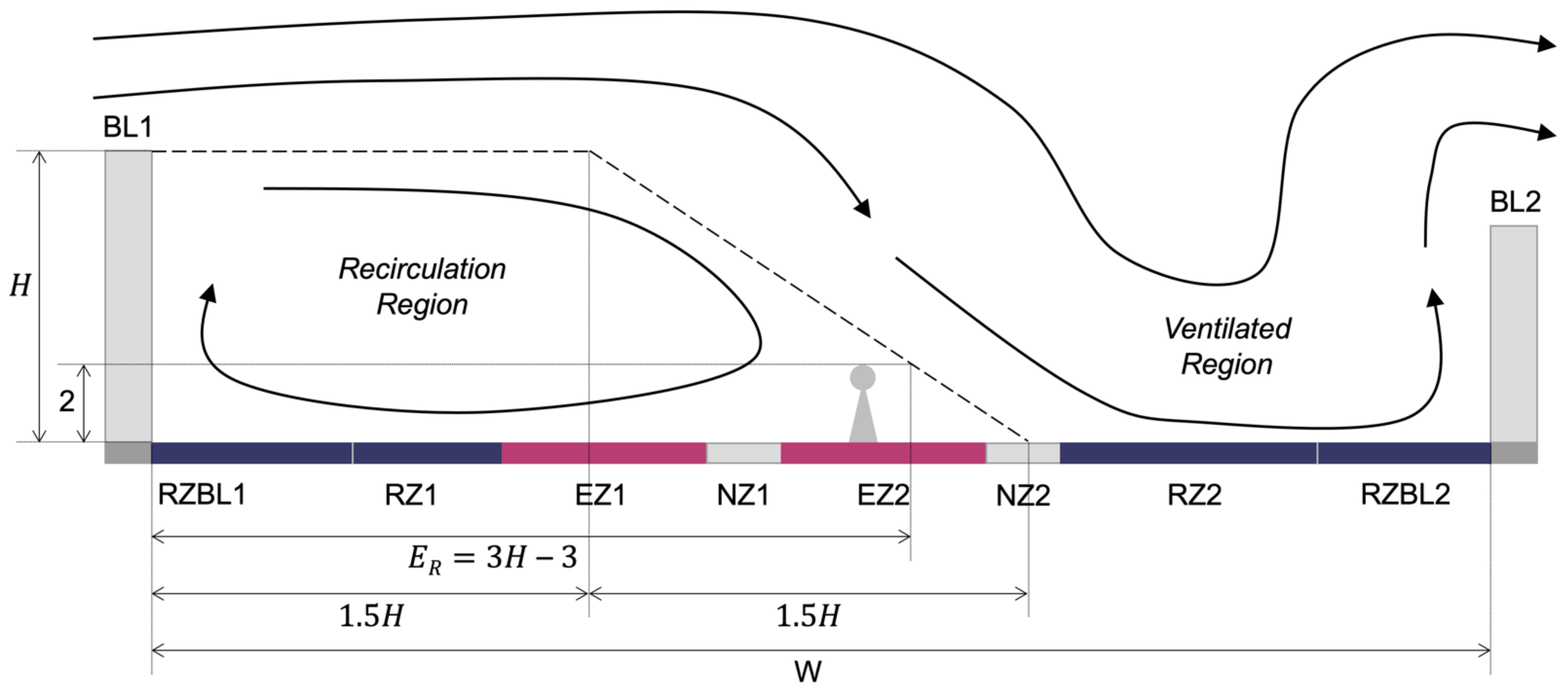
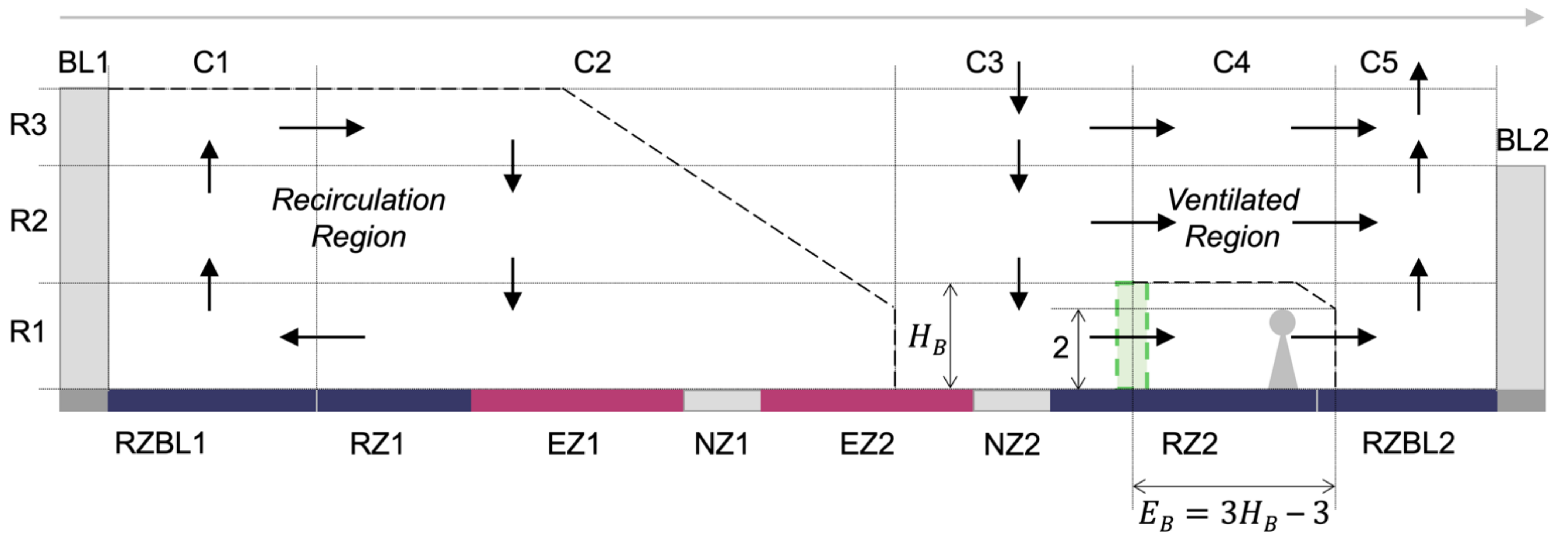
2.1.2. Two-Dimensional Street Model

The air quality code constitutes a two-dimensional model comprising five columns of variable width and three rows. The grid is laid out to represent the user-specified street section (cf. Figure 1). We limit the total number of boxes to 15 for reasons of practicality, trading-off spatial resolution against compute speed and ease of use. Whilst the code cannot readily accommodate additional rows and columns, we intend to increase its flexibility in due course.

The dimensioning of the three rows is as follows. The first row extends from the base of the street to the top of the proposed barrier (limited in the UI to being lower than the buildings either side); the second row stretches from the top of the barrier to the top of the shortest building (i.e., BL2 in Figure 1); and the third row extends from the top of the shortest building to the top of the tallest building (i.e., BL1 in Figure 1). If the buildings on both sides of the road are of equal height, the second and third rows are dimensioned so as to split the distance between the top of the barrier and the top of the buildings into two rows of equal height.

The model, like most atmospheric chemistry-transport models, calculates average NO₂ and PM_2.5 concentrations in each box. It cannot resolve gradients in concentration within any one box. The dimensioning of the columns therefore varies, as we aim to place column interfaces where we expect significant gradients in concentration, such as either side of the proposed barrier. Full details of the logic behind our dimensioning are provided in Supplementary Materials Section S2.

In the UI, the user is asked to specify the location of their street section and the compass direction looking down the street in that location (i.e., into the plane of the section). The location is used to select appropriate climatological wind data from the UK Meteorological Office [45] to describe the background wind conditions, which are used to approximate the wind speed and direction above the surrounding buildings, including variability therein. These data are then used to determine the air flow within the street. Based on 10 consecutive years of wind data, we calculate the fractions of time for which the wind blows in four 90° sectors: from left to right across the street, rendering BL1 in Figure 1 ‘upwind’ of the road; from right to left, rendering BL2 in Figure 1 ‘upwind’ of the road; and predominantly parallel with the road, either into or out of the plane of Figure 1. In each sector, we reduce the climatological wind conditions to a time-weighted mean across-street, or along-street, wind speed (see Supplementary Materials Section S3 for full details). We then use this wind speed to determine the air flow within the street, both with and without the proposed barrier. The changes in pollutant concentrations returned to the user via the UI are the time-weighted average changes in concentrations calculated in these four pairs of model calculations. Users of the offline code, however, are free to write out the absolute concentrations, and changes therein, calculated in each individual wind-sector scenario.

Figure 2 (adapted from [41]’s Figure 1a) illustrates the patterns of air flow expected within our example street section (W > 3 H) when the wind aloft blows from left to right; the arrows, illustrating the directions of air flow within the street, represent the ‘isolated roughness flow regime’ of [42]. Based on [41]’s formulation introduced in Section 1.3, the wind aloft creates a recirculation region in the wake of BL1—a trapezoidal region of overturning air extending a distance of about 3 H across the street. Within the recirculation region, the direction of air flow at the base of the street is reversed relative to that aloft whilst, in the ventilated region beyond, the direction of air flow matches that aloft. As we are primarily concerned with the exposure of people at pedestrian level (i.e., closest to vehicular sources of pollution), we slightly modify the extent of this recirculation region to reflect the distance for which a person up to 2 m tall is enclosed within it: Equation (1).

$$E_R=3\mathrm{H}-3$$

(1)

where $E_R$ is the horizontal extent of the recirculation region (m) downwind of a building of height, $\mathrm{H}$ (m).

Figure 3 illustrates the model grid adopted to represent this example street section. To resolve the circulation of air within the recirculation region, bringing air with emissions from EZ1 and EZ2 towards receptors in RZ1 and RZBL1, we require a minimum of two columns and two rows. Our dimensioning of rows always provides the latter, but we purposefully dimension the columns to provide the former; only when the recirculation region stops short of the first emission zone (i.e., is not expected to trap any emissions) do we opt not to resolve this circulation—representing it with a single column—and save a column for better use elsewhere in the street section. By default, the two columns spanning the circulation region (C1 and C2) are divided in line with the street boundary, as it is here that the user may wish to include an existing barrier, such as a garden wall or fence (not shown in Figure 3); see later. Note that the shape of the recirculation region, represented by a two-dimensional array of boxes, is thereby approximated to a rectangle.

The width of the third column (C3) is defined so its far edge aligns with the centre of the proposed barrier (the dashed green rectangle in Figure 3); the UI limits the user to proposing a single barrier between the kerb and the street boundary on one side of the road. Note, the same grid is used to determine the distribution of pollution, both with and without the proposed barrier. The partially isolated region of overturning air created in the immediate wake of the proposed barrier (see Section 1.3) is analogous to the recirculation region in the wake of a building, and so we calculate its extent (again truncated to reflect the region enclosing a person up to 2 m tall) according to Equation (2):

$$E_B=3H_B-3$$

(2)

where $E_B$ is the extent of the partially isolated region (m) downwind of a barrier of height, $H_B$ (m). In our example, where this region stops short of the building(s) on the far side, the remaining two columns (C4 and C5) are divided in line with its far edge. Whilst a fraction of air is expected to be diverted over the barrier, and around the partially isolated region in its wake, the remainder is expected to continue to pass through it.

The black arrows in Figure 3 indicate the directions (but not the magnitudes) of the advection velocities prior to introducing the barrier. The comparatively slow mixing of air between adjacent boxes is described by exchange velocities (not shown in Figure 3). Not only does the pattern of advection (and mixing) change when the wind aloft blows from right to left, but so does the dimensioning of the columns; this is described for our example street in Supplementary Materials Section S4. The two model grids adopted in these perpendicular wind scenarios are then reused for the parallel wind scenarios (i.e., when the wind aloft blows into or out of the plane of the street section). In these parallel scenarios, we assume there is no air flow perpendicular to the street (i.e., all advection velocities in the plane of the street section are equal to zero), and we need only account for the mixing of air via exchange velocities. To avoid introducing a bias linked to our choice of model grid, the changes in NO₂ and PM_2.5 concentrations due to the proposed barrier are calculated using both grids adopted in the perpendicular wind scenarios, and the results are given equal weight in jointly reflecting the changes estimated under parallel wind conditions aloft. Note that, as the positions of the five columns in the two grids may differ, the final weighted-average changes in concentrations returned to the user (reflecting climatologically variable wind conditions aloft) may span anywhere from five to ten columns.

2.1.3. Emissions

The user is required to specify either the emission rates for NO₂ and PM_2.5 (μg m⁻¹ s⁻¹), or the total vehicle movements (veh hr⁻¹), in each emission zone they include in their street section. If they choose to specify vehicle movements, these are converted to emission rates for NO₂ and PM_2.5 (μg m⁻¹ s⁻¹) based on UK vehicle fleet composition projections from the National Atmospheric Emissions Inventory (NAEI [46]; base year 2018), including hot and cold start emissions. The NO₂ emissions come solely from vehicle exhaust, whilst the PM_2.5 emissions have both exhaust and non-exhaust (brake, tyre and road wear) components. This conversion from vehicle movements to emissions can be easily adapted in the future to reflect the evolving UK vehicle fleet (e.g., increasing numbers of electric vehicles). Meanwhile, users with access to local emissions data (e.g., local authority officers with measured or modelled emissions for individual road links) are encouraged to use these. Irrespective of how they are specified, and the emissions associated with a particular emission zone are assumed to be distributed evenly across the full width of that zone. Where an emission zone straddles more than one column (see, e.g., EZ2 in Figure 3), its associated emissions are split between those columns in proportion to the fractions of the emission zone that lie within those column (i.e., in Figure 3, roughly 60% of emissions from EZ2 are ascribed to C2, whilst the remaining 40% are ascribed to C3).

2.1.4. Barriers

Currently, the user is limited to exploring the air quality impacts of a single barrier on one side of the street. That barrier can take a variety of forms, comprising a green barrier (e.g., a hedge) or grey barrier (e.g., a wall or a fence), with or without a parallel line of trees.

The green or grey barrier is essential to obstruct the horizontal flow of polluted air from vehicles to people at head height, and is therefore a requisite component and must be at least 2 m high. The user specifies, not only the dimensions of the barrier’s cross section, but also its precise position between the kerb and street boundary; the ‘percentage obstruction’ it poses (in the case of a green barrier, based on optical porosity at managed maturity, when in leaf; see, e.g., [47]); and, in the case of a green barrier, its seasonality (i.e., evergreen or deciduous).

The green or grey barrier may be accompanied by a line of trees to obstruct the flow of polluted air at a higher level, extending the height of overall barrier. The user specifies the dimensions and relative positions of the tree crowns (including their spacing along the street), in addition to the percentage obstruction they pose at managed maturity when in leaf, and their seasonality. The model calculates the percentage obstruction posed by the overall barrier: the height-weighted average of the percentage obstruction posed by each of its components (simply halved in the case of deciduous vegetation to account, crudely, for the time that vegetation is not in leaf). These components include any gap left between the green or grey barrier below and the tree crowns above. We use this overall percentage obstruction to modify the advection and/or exchange velocities between model boxes in the vicinity of the barrier; recall, the height of the first row is set to the height of the barrier, and we include a division between columns in line with its centre.

In the last section, we touched on the inclusion of existing barriers at street boundaries. These are currently limited to grey barriers (e.g., walls or fences), but we hope to extend the scope of the code in due course to include green barriers (e.g., garden hedges). When specified by the user, existing barriers are included in all model calculations, i.e., both with and without the proposed barrier. We thereby quantify the impacts of the proposed barrier on the distribution of pollutants within the street, in the context of the influence those existing barriers exert on the pattern of air flow therein. Where possible, just as for the proposed barrier, we try to include a division between columns in line with each existing barrier. We make some a priori assumptions, however, as to where they will have a relatively minor effect on the impact of the proposed barrier, and sometimes opt not to resolve their impacts on air flow in order to save a column for better use elsewhere within the street (see Supplementary Materials Section S2 for full details of the logic behind our dimensioning). In time, we hope to develop a more sophisticated treatment of advection that will offer greater resolution, and remove these a priori assumptions, without detrimentally affecting the compute time and the user’s engagement in an iterative design process.

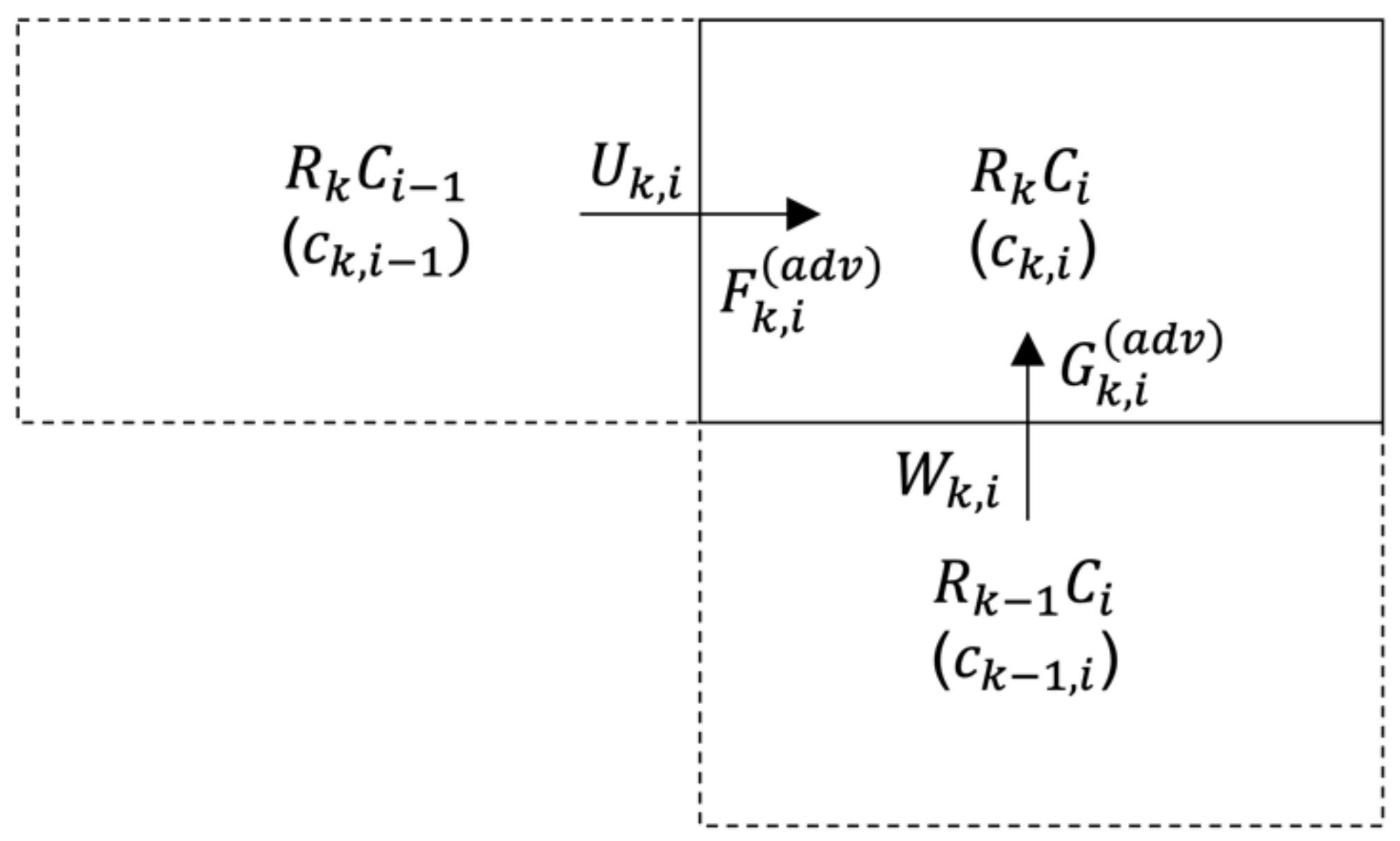
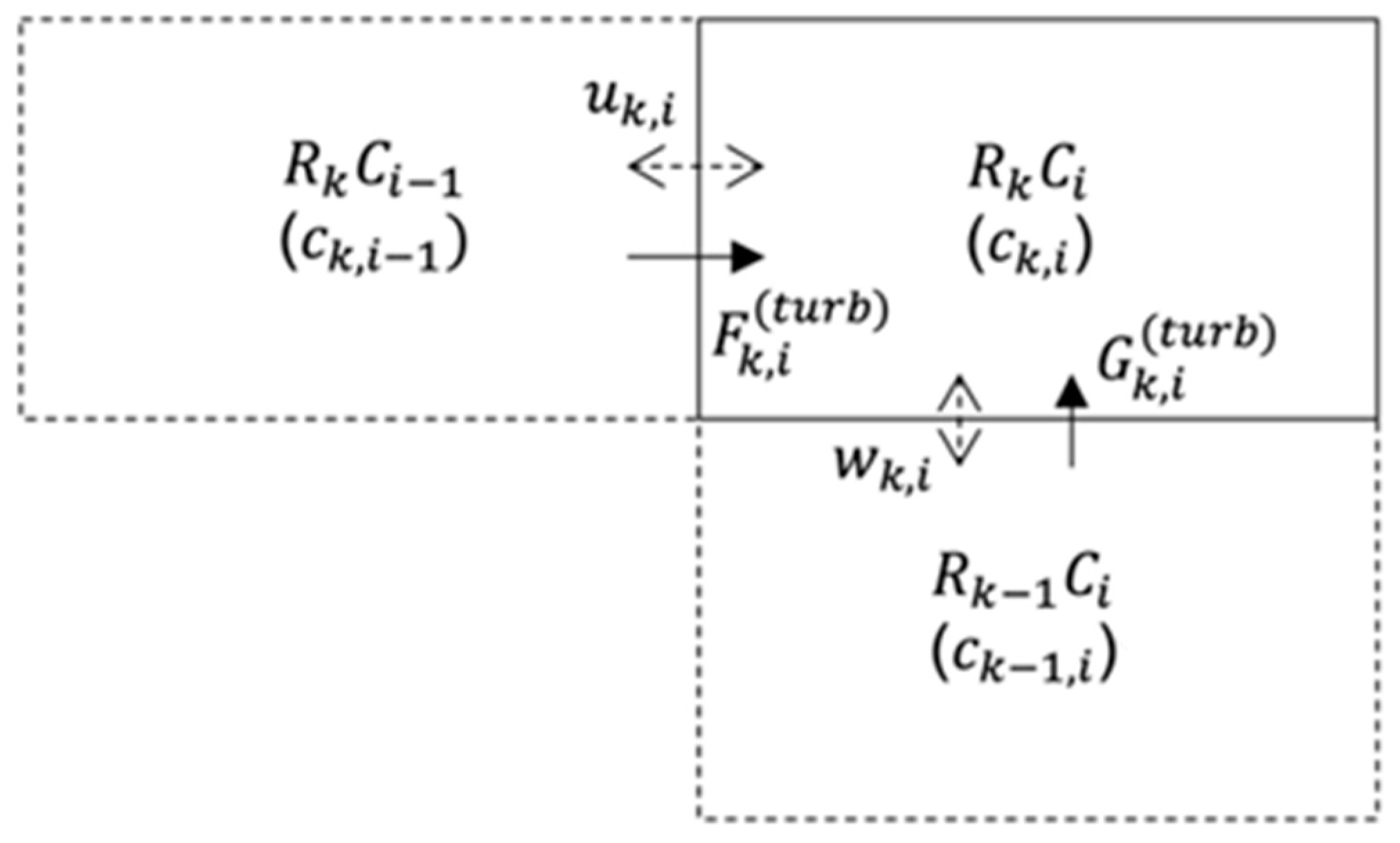
2.1.5. Mathematical Framework of the Model

The key to the model’s rapid estimation of steady-state pollutant concentrations in each wind-sector scenario (with and without the proposed barrier) is the prescription of advection and exchange velocities at each interface between its 15 boxes (five columns by three rows). This permits an analytical (as opposed to a numerical, or iterative) mathematical solution. Supplementary Materials Sections S5 and S6 explain how, for the purposes of the prototype GI4RAQ Platform, we estimate the advection and exchange velocities respectively, and modify these around barriers. The approaches we currently take are crude, and we intend to refine these in due course. Meanwhile, the mathematical framework will readily accept values calculated by more sophisticated and/or realistic means (e.g., using CFD models or experimental data). In preparation for the analytical computation of steady-state concentrations, the code converts the prescribed velocities into fluxes as outlined below.

For each pollutant, the horizontal and vertical advection velocities (describing the mean flow of air) are used to derive the horizontal and vertical advection fluxes according to Equations (3) and (4).

$$F_{k,i}^{\left(adv\right)}=\left\{\begin{array}{cc}{U}_{k,i}{c}_{k,i-1},& U_{k,i}\ge 0\\ U_{k,i}{c}_{k,i},& U_{k,i}<0\end{array}\right.$$

(3)

$$G_{k,i}^{\left(adv\right)}=\left\{\begin{array}{cc}{W}_{k,i}{c}_{k-1,i},& W_{k,i}\ge 0\\ W_{k,i}{c}_{k,i},& W_{k,i}<0\end{array}\right.$$

(4)

where, as schematically illustrated in Figure 4, the horizontal advection flux (per unit area—this applies to all definitions of flux thereafter) into box $R_k{C}_i$ (i.e., row k, column i) from box $R_k{C}_{i-1}$, $F_{k,i}^{\left(adv\right)}$, is positive where the horizontal advection velocity from box $R_k{C}_{i-1}$ to box $R_k{C}_i$, $U_{k,i}$, is positive (i.e., from left to right); $c_{k,i-1}$ and $c_{k,i}$ are the pollutant’s concentrations in boxes $R_k{C}_{i-1}$ and $R_k{C}_i$, respectively. Likewise, the vertical advection flux into box $R_k{C}_i$ from box $R_{k-1}{C}_i$, $G_{k,i}^{\left(adv\right)}$, is positive where the vertical advection velocity from box $R_{k-1}{C}_i$ to box $R_k{C}_i$, $W_{k,i}$, is positive (i.e., upwards); $c_{k-1,i}$ and $c_{k,i}$ are the pollutant’s concentrations in boxes $R_{k-1}{C}_i$ and $R_k{C}_i$ respectively.

Likewise, for each pollutant, the horizontal and vertical exchange velocities (describing the turbulent mixing, or dispersion, of air) are converted to net horizontal and vertical turbulent fluxes according to Equations (5) and (6). The dependence of each net turbulent flux on the pollutant’s concentration gradient follows Fick’s law [48].

$$F_{k,i}^{\left(turb\right)}=u_{k,i}\left(c_{k,i-1}-c_{k,i}\right)$$

(5)

$$G_{k,i}^{\left(turb\right)}=w_{k,i}\left(c_{k-1,i}-c_{k,i}\right)$$

(6)

where, as schematically illustrated in Figure 5, the net horizontal turbulent flux into box $R_k{C}_i$ from box $R_k{C}_{i-1}$, $F_{k,i}^{\left(turb\right)}$, due to horizontal exchange velocity, $u_{k,i}$, is positive where the concentration gradient slopes down from box $R_k{C}_{i-1}$ to box $R_k{C}_i$ (i.e., from left to right); and the net vertical turbulent flux into box $R_k{C}_i$ from box $R_{k-1}{C}_i$, $G_{k,i}^{\left(turb\right)}$, due to vertical exchange velocity, $w_{k,i}$, is positive where the concentration gradient slopes down from box $R_{k-1}{C}_i$ to box $R_k{C}_i$ (i.e., upwards).

At steady state, the combination of the advection and turbulent fluxes of each pollutant must equate to the ‘emission’ fluxes of that pollutant, where the latter include the user-specified emissions into the street from emission zones at its base (see Section 2.1.3), the additional fluxes into the street associated with the entrainment of polluted air aloft (characterised by user-specified background pollutant concentrations) and the fluxes out of the street associated with the expulsion of air into the region aloft. Using vector notation to cover the entire two-dimensional array of model boxes, we can express the combination of advection and turbulent fluxes as the product of a matrix, $A$ (a function of advection and exchange velocities, $U_{k,i},W_{k,i}, u_{k,i}$ and $w_{k,i}$; see Equations (3)–(6)) and a vector of pollutant concentrations, $\overrightarrow{C}$. We can also express the combination of emission fluxes as a vector, $\overrightarrow{D}$, and equating one to the other to reflect steady state yields Equation (7).

$$A\overrightarrow{C}=\overrightarrow{D}$$

(7)

Rearranging Equation (7) yields Equation (8) that allows us to calculate steady-state concentrations, $\overrightarrow{C}$, via inverse matrix, $A^{-1}$ and emission vector, $\overrightarrow{D}$. For further information, please see Supplementary Materials Section S7.

$$\overrightarrow{C}=A^{-1}\overrightarrow{D}$$

(8)

2.2. First Tests of Model Performance

To test the performance of our simple box model, we have used it to estimate the absolute concentrations of pollutants, and the changes produced by roadside barriers, measured in well-constrained real-world and wind tunnel environments. We exploit the established dataset of measurements at the Automatic Urban and Rural Network (AURN) site on Marylebone Road, London, UK (latitude: 51.522530° N, longitude: −0.154611° E) to test the model‘s capacity to estimate the right order of magnitude of NO₂ and PM_2.5 concentrations in a highly trafficked urban street canyon ($\mathrm{W}\approx 1.7\mathrm{H}$). We subsequently emulate a wind tunnel study [49], in which tracer-doped air was used to assess the impacts of introducing roadside barriers in a street of similar aspect ratio ($\mathrm{W}=2\mathrm{H}$), under both parallel and perpendicular wind conditions aloft. Finally, we use the model to estimate the changes in NO₂ concentrations measured behind a roadside barrier introduced in a real open-road environment [50] ($\mathrm{W}>>3\mathrm{H}$). Below, we describe the model setups used in these direct comparisons between model and measurements.

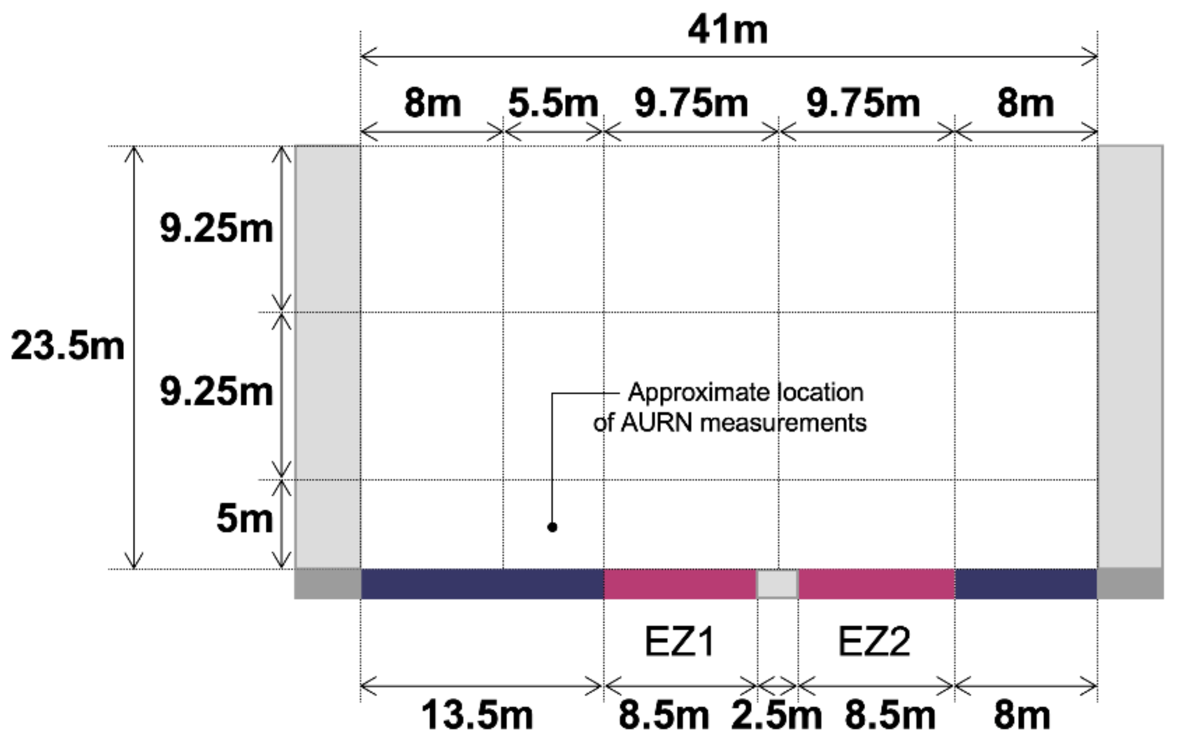
2.2.1. Absolute Concentrations in a Real Street Canyon

The AURN site, run by the UK Government’s Department for Environment, Food and Rural Affairs (DEFRA), is located on the southern pavement of Marylebone Road, which runs roughly east–west in north London. This is a well-known pollution hot spot, in which DEFRA’s reference analysers provide hourly measurements of NO₂ and PM_2.5 concentrations. Here, we use the model to estimate the annual mean concentrations of NO₂ and PM_2.5 in 2012—chosen on account of the recent publication of a simulation of 2012 annual mean NO₂ concentrations, across the entire street section in this location, using an ‘advanced street canyon air pollution model’ [51].

The street section’s dimensions are estimated from Ordnance Survey MasterMap products and Google Maps ‘street view’, and compare well with those adopted in previous studies, e.g., [52]; we ascribe the same height of 23.5 m to the buildings on both sides of the street. The street section’s dimensions, and the model grid we apply, are illustrated in Figure 6, looking roughly west (254°) along the street; emission zones EZ1 and EZ2 thus represent westbound and eastbound carriageways, respectively.

The emissions of NO₂ and PM_2.5 from vehicles within the street (an average of 77,180 vehicles per day in 2012 [53]) are specified based on the 2013 London Atmospheric Emissions Inventory (LAEI) [54]. PM_2.5 emissions are taken directly from the LAEI (20.2 µg m⁻³ s⁻¹ and 18.8 µg m⁻³ s⁻¹ are ascribed to EZ1 and EZ2, respectively), whilst NO₂ emissions are estimated based on LAEI emissions of NO_x (i.e., NO + NO₂). The fraction of NO_x emissions that constitute direct emissions of NO₂ is often assumed to be around 10% [55,56,57], although, in practice, it is highly dependent on the local vehicle fleet composition [58]. As our model treats NO₂ as a passive tracer, we must increase this fraction to account for the rapid conversion of some directly emitted NO to NO₂ via ozone titration. We assume that the total fraction of NO_x emissions, directly emitted as NO₂ or emitted as NO and rapidly converted to NO₂, is equal to the ratio of NO₂ to NO_x concentrations (i.e., [NO₂]/[NO_x]) typically observed in a similar urban environment. At the annual mean concentration of NO_x measured at the AURN site in 2012 (313.2 µg m⁻³), four empirical relationships used by UK air quality regulators yield [NO₂]/[NO_x] ≈ 24%, 27%, 31% and 19% ([59,60,61,62], respectively). Treating 25% of NO_x emissions as NO₂, we ascribe NO₂ emission rates of 137.9 µg m⁻³ s⁻¹ and 113.3 µg m⁻³ s⁻¹ to EZ1 and EZ2 respectively. Meanwhile, the annual mean background pollutant concentrations in this location are estimated using DEFRA’s UK Air Information Resource [63]: 40.03 µg m⁻³ NO₂ and 17.15 µg m⁻³ PM_2.5 for 2012.

The background wind conditions are derived from 2012 hourly observations of wind speed and direction at the nearest UKMO station (Heathrow), courtesy of the MIDAS Open archive [45]. As outlined in Section 2.1.2, these are first reduced to the fraction of time the wind blows in each of four 90° sectors relative to the street, and the mean across-street or along-street wind speed in each: 19.9% left to right across the street at 4.02 m s⁻¹; 18.3% from right to left across the street at 2.62 m s⁻¹; and a total of 61.7%, either into or out of the plane of the street section, at 3.96 m s⁻¹. We model the concentrations of NO₂ and PM_2.5 subject to each of these wind scenarios, before calculating a time-weighted average.

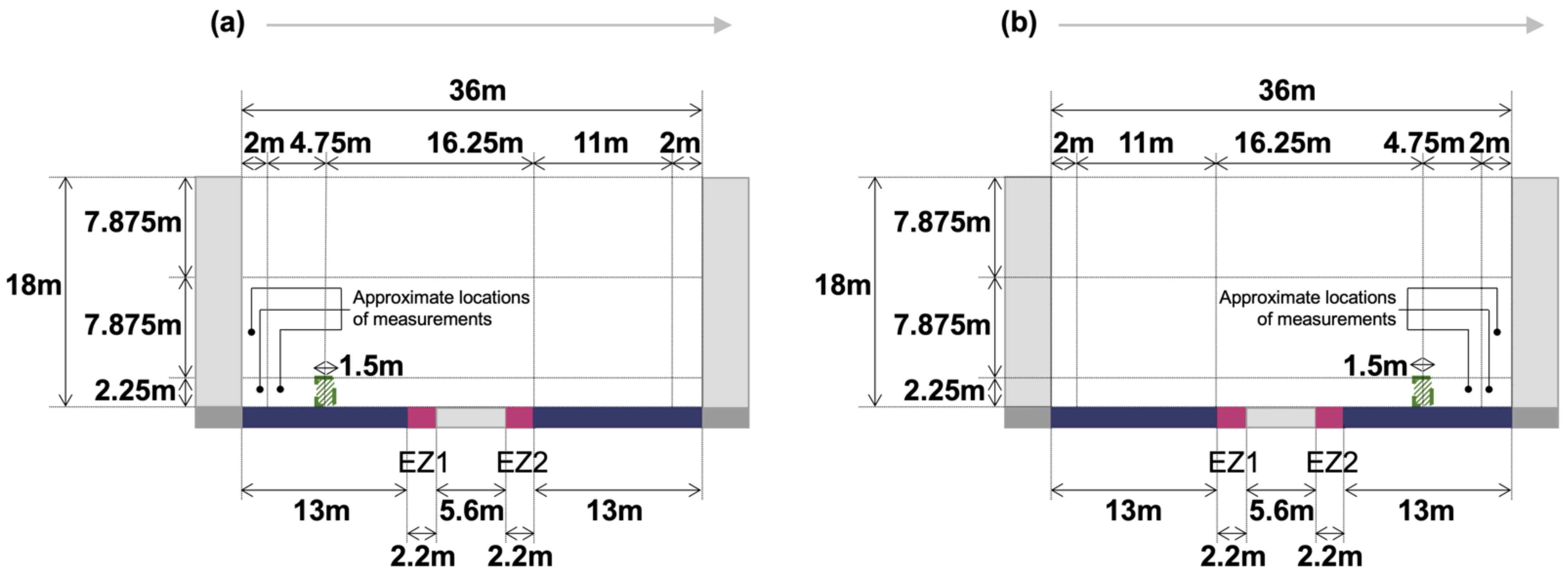
2.2.2. Impacts of Roadside Barriers in a Simulated Street Canyon

The impacts of introducing roadside barriers in a street canyon similar to Marylebone Road (W = 2 H) have been explored in a wind tunnel study, using a 1:150 scale model [49]. Here, we attempt to reproduce the changes in pollutant concentrations measured half-way along the street, mainly at a height equivalent to 1.5 m, on introducing 2.25 m-tall barriers between the road and the adjacent buildings. Authors in [49] made these measurements under, separately, parallel and perpendicular wind conditions aloft. Whilst the original study measured the impacts of simultaneously adding barriers either side of the road, we are limited to modelling the impacts of introducing one barrier at a time. Under perpendicular wind conditions, therefore, we perform separate calculations for the addition of a barrier (a) upwind and (b) downwind of the road; the scaled-up street dimensions, and resulting model grids, are illustrated in Figure 7; for consistency, we adopt the same model grids for the parallel-wind calculations. These grids ensure that the region behind each barrier is divided into two boxes, enabling us to resolve differences between the two locations in which measurements were made at the base of the street behind the barrier (see Figure 7).

In the wind tunnel study, 7006.5 cm³ min⁻¹ doped air (928 ppmv SF₆) was introduced via four line sources, each 1.42 m long (running parallel with the street and counter-sunk into the base of the scale model). They were divided into two pairs, each pair representing a separate carriageway. We emulate this setup in our model with two emissions zones, EZ1 and EZ2. Viewed in cross-section (Figure 7), each emission zone extends from the position of one line source, to the position of its paired line source, and is ascribed an emission rate of 232.1 mg m⁻¹ s⁻¹ SF₆. We assume the background SF₆ concentration is zero.

The wind conditions in the model are constrained by assuming the wind speed at the height of the buildings either side—either parallel with, or perpendicular to, the street—is equal to the wind speed achieved in the wind tunnel (4.65 m s⁻¹).

Finally, we must specify the percentage obstruction posed by the barrier in our model (the green shaded rectangles in Figure 7a,b). Two types of barriers were employed by [49] (pore volume fractions of 96.1% and 94.5%). We perform a range of calculations specifying obstructions of 50%, 70% and 90%.

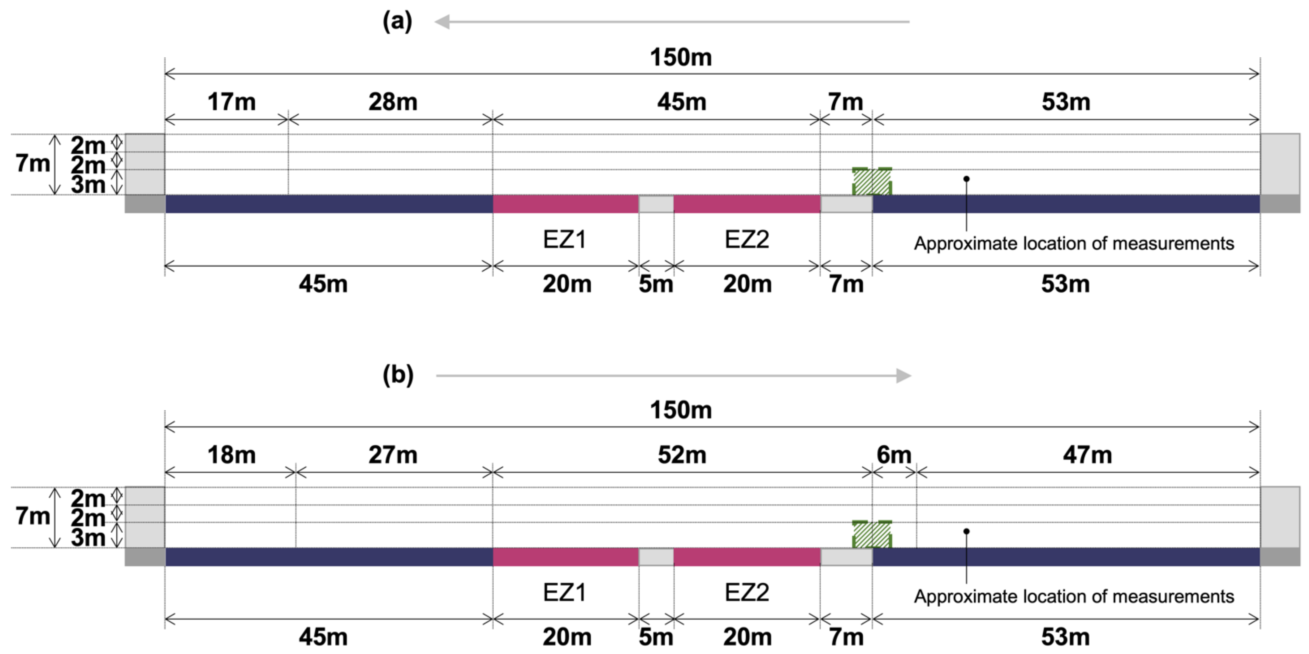
2.2.3. Impact of a Barrier beside a Real Open Road

The impact of a barrier on roadside NO₂ concentrations has been assessed beside an open road (W >> 3 H), Interstate-280 (Woodside, CA, USA) [50]. Here, we attempt to reproduce the percentage difference between the mean NO₂ concentrations measured in this assessment (i) behind a line of bushes (3 m tall and 5 m wide in cross section) and (ii) in an adjacent clearing (equidistant from the road). Figure 8 illustrates the cross-section of this open-road environment, looking roughly southeast along the road (130°), with dimensions estimated from Google Maps satellite and street views; also illustrated are the model grids adopted when the barrier lies (a) upwind and (b) downwind of the road, relative to the wind aloft; as before, we reuse these grids for the parallel-wind calculations.

We have no direct means of constraining the emissions of NO₂ from Interstate-280 during [50]’s summer study period. We can, however, specify a background NO₂ concentration (7 µg m⁻³) with reference to measurements at the Redwood City monitoring station [64], located roughly 3 km to the northeast of the site. We simply halve the Jun–Aug 2017 mean NO₂ concentration measured at this urban station, in view of the study site’s proximity to the Pacific Ocean (10 km to its south and west); background NO₂ concentrations during southerly and westerly winds would be negligible compared to the urban monitoring site. We then tune the emissions of NO₂ (40.3 mg m⁻¹ s⁻¹ from each side of the dual carriageway, represented by emission zones EZ1 and EZ2 in Figure 8) to determine an NO₂ concentration at the measurement site in the absence of a barrier (16.62 µg m⁻³) close to the reported mean measurement in the clearing (16.83 µg m⁻³, based on [50]’s Table S1).

The background wind conditions in the model are constrained using the wind speeds and directions measured in situ throughout the measurement period (at approximately half the height of the buildings either side); see [50]’s Figure 3 and Table 2. Like for Marylebone Road, these are first reduced to the fraction of time the wind blows in each of four 90° sectors relative to the street, and the mean across-street or along-street wind speed in each at a reference height of 10 m (scaling the in situ wind speed measurements by a factor of 1.5): 29.0% left to right across the street at 1.88 m s⁻¹; 12.5% from right to left across the street at 1.58 m s⁻¹; and a total of 58.5%, either into or out of the plane of the street section, at 1.64 m s⁻¹. We then model the concentrations of NO₂ throughout the street section, subject to each wind scenario, both with and without the barrier. Having calculated the percentage changes in NO₂ concentration due to the barrier in each wind scenario, we finally calculate the time-weighted average changes in NO₂ concentration.

Regarding the barrier, we specify a percentage obstruction of 75%, based directly on the 25% (optical) porosity of the bushes (‘Stop 2′) estimated in [50]’s Table 1.

3. Results

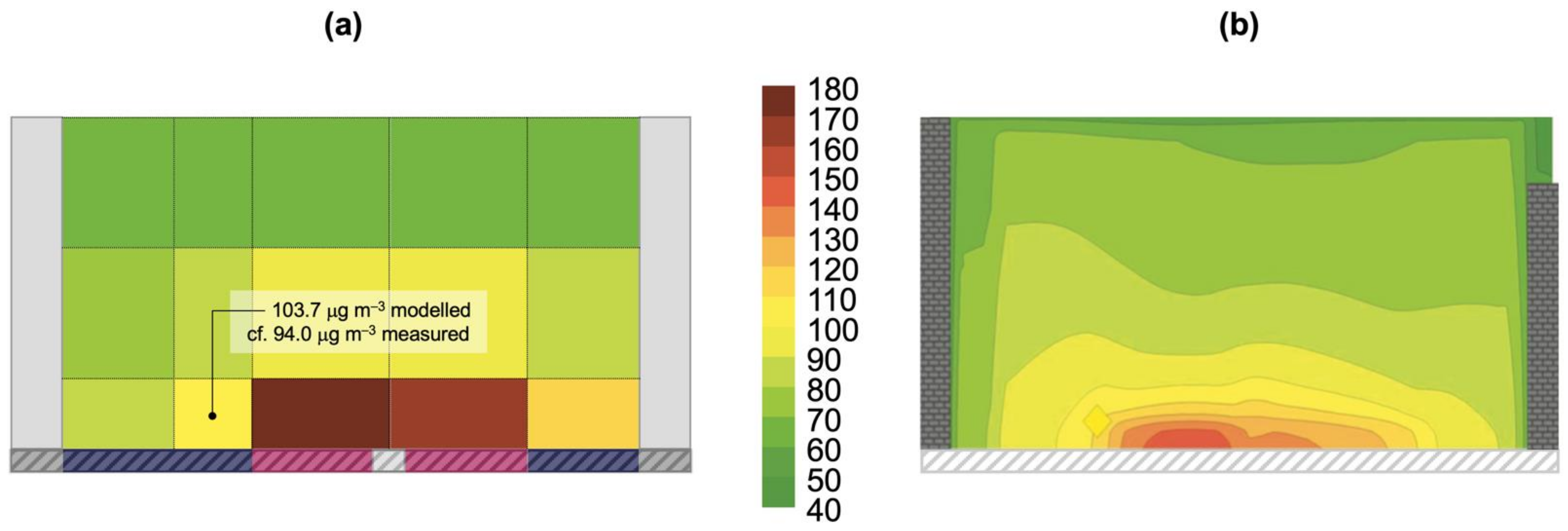
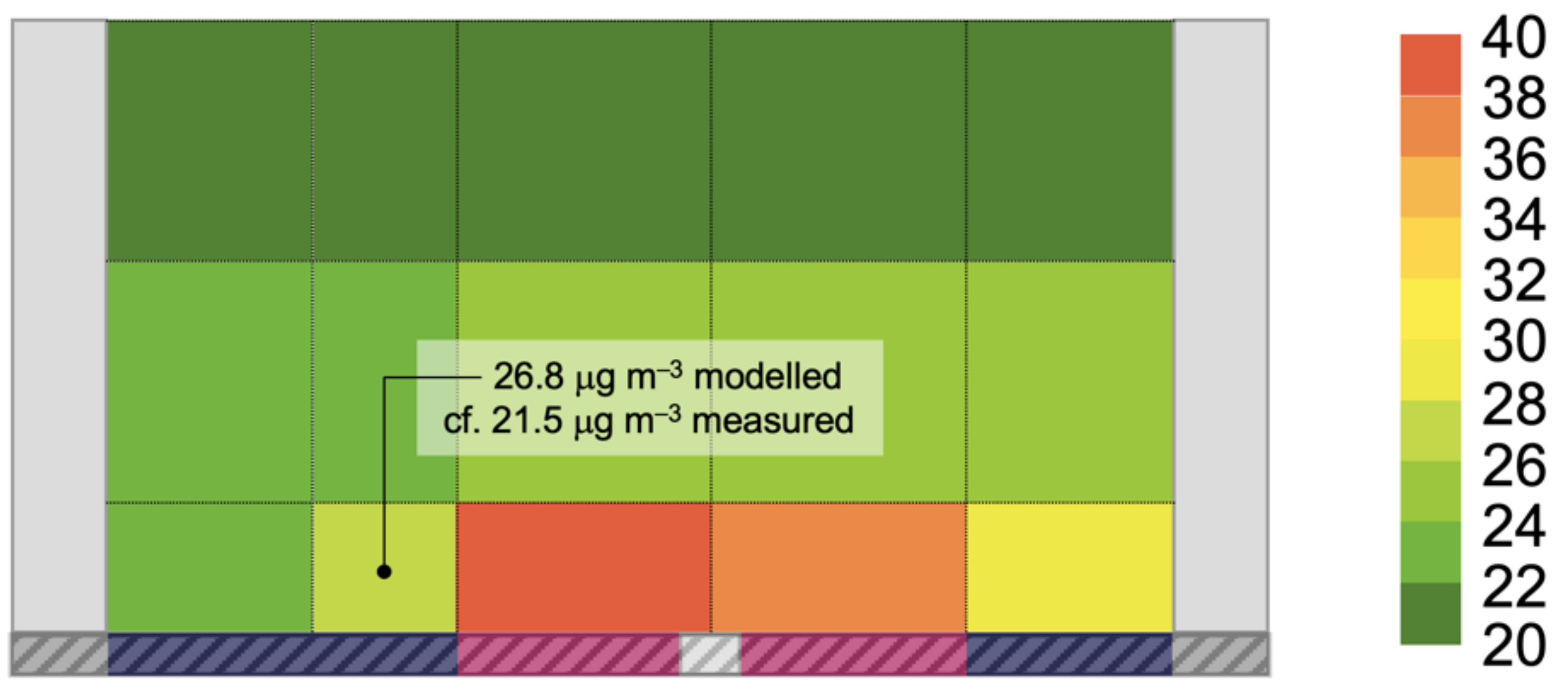
3.1. Absolute Concentrations in a Real Street Canyon

Figure 9 illustrates the 2012 annual mean distribution of NO₂ we modelled in a cross-section ($\mathrm{W}\approx 1.7\mathrm{H}$) of Marylebone Road, London, at DEFRA’s AURN site (a); and a reproduction of [51]’s Figure 7, showing their recent simulation of annual mean NO₂ at the same site, in the same year, using an ‘advanced street canyon air pollution model’ (b). Where indicated in the figure, our model yielded an annual mean NO₂ concentration of 103.7 mg m⁻³, which is 10% higher than the 94.0 mg m⁻³ measured. Comparing the left- and right-hand sides of the figure, our model yielded a similar, qualitative annual mean distribution of NO₂ to [51]’s simulation, but yielded approximately 10% higher NO₂ concentrations in the lower half of the street. We note that their model is much more sophisticated than our simple two-dimensional box model, and refer the reader to [51] for full details.

As a sensitivity test, we repeated our model calculations, including only direct emissions of NO₂ (assumed to be 10% of total NO_x emissions; see Section 2.2.1) and omitting the effects of NO-to-NO₂ conversion via ozone titration. This yielded a 37% lower annual mean NO₂ concentration of 65.5 µg m⁻³. We also tested the validity of otherwise treating NO₂ as a passive tracer (i.e., assuming the influence of NO_x sinks can be neglected) by using the same model framework to estimate the annual mean concentration of NO_x at this site. Setting emissions to 100% of the LAEI’s [54] values for NO_x (551.6 µg m⁻³ s⁻¹ in EZ1 and 453.2 µg m⁻³ s⁻¹ in EZ2) and the background concentration to 75.5 µg m⁻³, based on [63], the model yielded an annual mean NO_x concentration of 330.3 µg m⁻³, just 5% over the 313.2 µg m⁻³ measured.

The annual mean distribution of NO₂ illustrated in Figure 9a is the time-weighted average of the NO₂ distributions we model in four separate wind-sector scenarios. Disaggregating these, we find that the model reproduced much of the observed dependence of NO₂ measurements at the AURN site on wind direction: an elevated mean concentration when the wind blows from left to right across the street (southerly winds) of 119.8 mg m⁻³ cf. 110.9 mg m⁻³ measured; a lower mean concentration when the wind blows from right to left across the street (northerly winds) of 77.9 mg m⁻³ cf. 62.5 mg m⁻³ measured; and an intermediate mean concentration when the wind blows in either direction along the street (easterly or westerly winds) of 106.2 mg m⁻³ cf. 98.2 mg m⁻³ measured.

Finally, Figure 10 illustrates the 2012 annual mean distribution of PM_2.5 we modelled at this site. It was qualitatively similar to our modelled distribution of NO₂, with elevated concentrations in the vicinity of emission zones at the base of the street canyon, decaying towards the specified background concentration at its top. The concentrations of PM_2.5 were lower than those of NO₂, however, due its lower emissions and lower background concentration. Where indicated in the figure, the model yielded an annual mean PM_2.5 concentration of 26.8 mg m⁻³, which is 25% higher than the 21.5 mg m⁻³ measured. Our simple model employed a single, annual mean background PM_2.5 concentration (irrespective of wind direction; discussed in Section 4). As a sensitivity test, we repeated the model calculations with a 25% lower background concentration (12.86 cf. 17.15 µg m⁻³). This yielded an annual mean PM_2.5 concentration of 22.5 µg m⁻³, just 5% over the 26.8 µg m⁻³ measured.

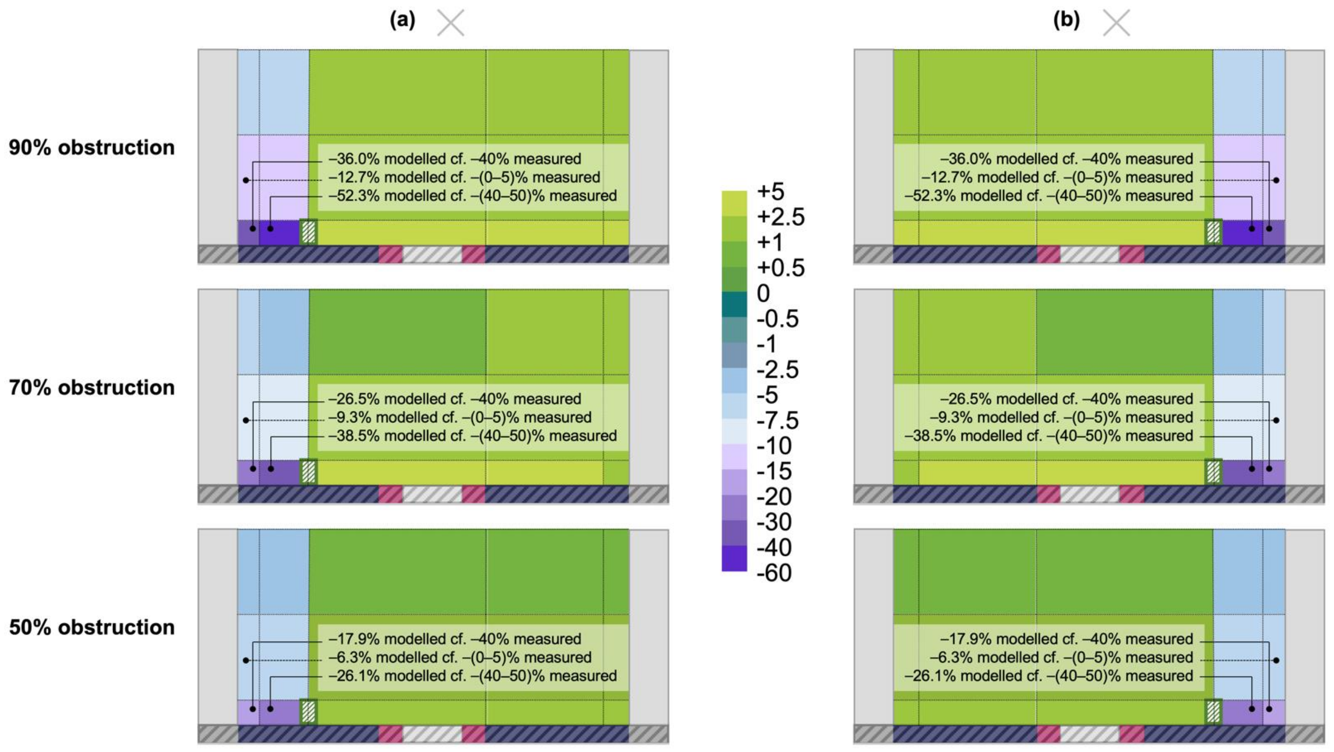
3.2. Impact of Roadside Barriers in a Simulated Street Canyon

Figure 11 illustrates the percentage changes in SF₆ concentration we modelled on introducing a roadside barrier (50, 70 or 90% obstruction) in a street canyon ($\mathrm{W}=2\mathrm{H}$) under parallel wind conditions aloft, as we seek to emulate [49]’s wind tunnel study. Under parallel wind conditions, the impacts of introducing a barrier on the left were a mirror image of the impacts of introducing one on the right, but this symmetry broke down when we later looked at the impacts under perpendicular wind conditions. Best agreement between the percentage reductions we modelled behind the barrier at the base of the street, and those measured by [49] (taken from their Figure 9; values of ‘Dc⁺_rel floor’ at x/H= 0.834 and 0.917, y/H = 0) was achieved with a 90% obstruction. Here, we modelled a 52% reduction in pollution immediately behind the barrier cf. 40–50% measured; and a 36% reduction closer to the adjacent building cf. 40% measured. Our modelled reductions dropped to 26% immediately behind the barrier and 18% beside the building when we specified a 50% obstruction, but remained of the right order of magnitude. Meanwhile, at the façade of the adjacent building, a third the distance from the bottom to the top of the street canyon, we modelled reductions of 6–13% with barriers of 50–90% obstruction. These are somewhat greater than the 0–5% reductions measured (taken from [49]’s Figure 9; value of ‘Dc⁺_rel wall’ at y/H = 0, z/H = 0.333) but nevertheless of the right order of magnitude.

Figure 12 illustrates the percentage changes in SF₆ concentration we model on introducing a roadside barrier (50, 70 or 90% obstruction) in the simulated street canyon, (a) upwind and (b) downwind, relative to perpendicular wind conditions aloft. Qualitatively, like the measurements, the model yields reductions in concentration behind the barrier, both at the base of the street and a third the way up the adjacent building’s façade. However, the magnitudes of the reductions we model are much lower than those measured by [49] (taken from their Figure 5; values of ‘h_h = 2.25 m, l_h = 1.67 m^−1′ and ‘h_h = 2.25 m, l_h = 3.34 m^−1′ in positions f_A/B10-1, f_A/B10-2 and w_A/B4-4). When the barrier is downwind, we model a maximum reduction of 12.1% (immediately behind a barrier of 90% obstruction) compared to a measured reduction of 32–54%. When the barrier is upwind, the percentage reductions we model are at least two orders of magnitude lower, effectively zero, whilst [49]’s measured reductions range from 2 to 44%. We discuss the likely cause of these underestimates, relative to [49]’s idealised wind tunnel simulation, in Section 4.

3.3. Impact of a Barrier beside a Real Open Road

Figure 13 illustrates the percentage changes in NO₂ concentration we modelled on introducing a roadside barrier in an open-road environment ($\mathrm{W}\gg 3\mathrm{H}$), for comparison with [50]. These are the time-weighted average changes in NO₂ we modelled in four separate wind-sector scenarios. In this figure, we present the modelled results subject to the original model grids (Figure 8), and an alternative model grid (discussed below). Employing the original model grids, we calculated a 2.1% reduction, where [50] measured a reduction of 11.8%. Note, however, that we calculated a 9.2% reduction very close to the measurement site, but limited to the immediate wake of the barrier (when the wind blows from left to right as pictured). Recall from Section 2.1.2 that, when a barrier is introduced in a ventilated region, we attempt to resolve the extent of the partially isolated region of overturning air created in its immediate wake. With just one column remaining, however, the modelled impact of the barrier further to the right (a 2.1% reduction) reflects the average change in NO₂ concentration we calculate across the full 47 m remaining between this partially isolated region and the building on the right-hand side of Figure 13. In this instance, the single remaining column does not permit us to resolve the return of air flow forced up and over the barrier (via the middle row of boxes) to the lowermost row of the model prior to expulsion up, out of the street.

When we repeated the model calculations, prioritising resolution of this pattern of air flow on the right-hand side (at the expense of resolution on the left-hand side, where the changes in NO₂ are more homogenous), we obtained the results illustrated at the bottom of Figure 13. Subject to the alternative model grids, we then modelled an 11.9% reduction in the immediate wake of the barrier, and a 17.0% reduction at the measurement site. Whilst we did not precisely reproduce the measured reduction in either case, we modelled reductions of the right order of magnitude close to the measurement site in both cases. It is also reassuring that the overall picture of the modelled changes in NO₂ across the whole of this open-road environment was relatively insensitive to the model grids employed. In both cases, we modelled increases of less than 2.5% on the far side of the dual carriageway from the barrier (i.e., on the left of Figure 13); increases of 2.5–10% in the top and bottom model rows in the vicinity of the road, and between the road and barrier; more marked increases of 15–40% in the middle row, where polluted air is forced up and over the barrier (when the wind blows from left to right); and marked decreases in the lowermost row, in the wake of the barrier, as previously described, relaxing towards zero-change in the region above.

4. Discussion and Conclusions

These first tests of the model’s performance are promising, especially when we recall that the prototype GI4RAQ Platform is a scoping tool, applicable to a wide variety of streets, not designed to predict pollutant concentrations in one particular type. The model reproduces the annual mean concentrations of NO₂ and PM_2.5 beside Marylebone Road, London, to within 10% and 25% respectively. Moving from absolute pollutant concentrations to the impacts of roadside barriers, the focus of our planning tool, the model exhibits the correct qualitative changes in pollutant concentrations observed in street-canyon and open-road environments, and it estimates changes of approximately the right size in these environments, except for the street canyon under perpendicular wind conditions aloft.

There are limitations to the current model, and future developments should increase its predictive skill and scope. We have made the model open source to engage the wider research community in its continued development.

4.1. Modelling Absolute NO₂ Concentrations

The model’s estimates of NO₂ concentrations beside Marylebone Road exhibit good agreement with observations, not only in terms of the 2012 annual mean, but also underlying variability with respect to wind direction. Furthermore, our assumption that NO_x sinks (deposition and chemical transformation) can be neglected in our simple model framework appears to be valid: it reproduces the observed 2012 annual mean concentration of NO_x here to within 5%. The model’s estimates of NO₂ concentrations are, however, sensitive to the fraction of NO_x emissions treated as NO₂ emissions: it yields a 37% lower annual mean concentration at this site when we include only directly-emitted NO₂; hence, is sensitive to the additional fraction of NO_x emissions assumed to be emitted as NO but rapidly converted to NO₂ via ozone titration. This fraction can be estimated, as we have done, using empirically derived [NO₂]/[NO_x] relationships (e.g., [59,60,61,62]) and the appropriate value of [NO_x] in the location of interest (available from, e.g., DEFRA’s UK Air Information Resource [63]). However, these relationships are approximate; they reflect the nature of the environments (e.g., ozone concentration) where the measurements of [NO₂] and [NO_x], on which they are based, were made and, therefore, yield somewhat different values of [NO₂] for a given value of [NO_x].

It will be challenging for the average user of the prototype GI4RAQ Platform to pick a suitable relationship for their site, and consider the inherent uncertainty in the fraction of NO_x emissions they treat as NO₂. A priority future development is, therefore, the inclusion of a photochemistry scheme to calculate [NO₂]/[NO_x] for that site, subject to its latitude, affecting the rate of NO₂ photolysis, and the ambient ozone concentration (e.g., from [63]), affecting the rate of NO-to-NO₂ conversion. Modelling NO_x (cf. NO₂) as a passive tracer, and using the photochemical scheme to disaggregate NO_x into NO and NO₂, the user will be able to specify NO_X emissions (readily available to them) and obtain estimated changes in NO₂ concentrations (most pertinent to local air quality management).

4.2. Modelling Absolute PM_2.5 Concentrations

Roadside PM_2.5 concentrations reflect both background PM_2.5 concentrations, due to regional-scale emissions and chemical transformations, and proximate PM_2.5 emissions (e.g., from vehicles). Just a few metres from the kerb, only around 20% of PM_2.5 (mass) concentrations is attributable to nearby vehicles (e.g., [65]), compared with roughly 60% of NO₂ concentrations [66]. The lower fraction of PM_2.5 attributable to local sources reflects its longer atmospheric lifetime and, consequently, its ability to travel further from point of emission to point of removal from the air. For instance, high PM_2.5 concentrations in the UK are often associated with the import of air from continental Europe [65]. The dependence of PM_2.5 in a given location to the history of air arriving in that location challenges our simple modelling approach, particularly our use of a single, annual mean background PM_2.5 concentration. This simplification could explain the model’s 25% overestimation of annual mean roadside PM_2.5 on Marylebone Road, as this background PM_2.5 concentration determines the minimum roadside concentration the model can yield (subject to zero vehicular emissions and/or perfect ventilation); reducing the background concentration by 25% reduced the modelled annual mean concentration to within 5% of that observed.

The current approach neglects the potential correlation between background PM_2.5 concentration and wind direction aloft, but was chosen to ensure the Platform only re-quires information readily available to its users (e.g., from [63]). Even with such a crude approximation, the model easily achieves the level of agreement (a factor of two) sought by [51] in their recent validation of an ‘advanced street canyon air pollution model’ for NO₂. Furthermore, we model close to the observed annual mean concentrations of NO₂ and NO_x in the same location, drawing on the same emissions dataset [54], and a qualitatively similar annual mean distribution of NO₂ throughout the cross-section of the street canyon to [51]. This suggests our overestimation of PM_2.5 is not primarily due to a structural problem in the model, which would affect both NO_x and PM_2.5 equally.

4.3. Roadside Barriers in Street Canyons under Perpendicular Wind Conditions

Exposing a 1:150 scale-model of a street canyon to contrasting wind conditions in a wind tunnel, [49] measured 40–50% reductions in pollutant concentrations behind roadside barriers under parallel wind conditions, and only slightly lower reductions under perpendicular wind conditions. Specifying a barrier of 90% obstruction, our model yielded very similar reductions of 36–52% under parallel wind conditions, but reductions of just 0–12% under perpendicular ones.

In our perpendicular-wind calculations, advection velocities remained unaltered on introducing a barrier. As outlined in Supplementary Materials Section S5, we currently only divert a fraction of the mean air flow around barriers introduced in ventilated regions (cf. recirculation regions encountered, for example, in street canyons). In both the parallel and perpendicular-wind calculations, however, the turbulent mixing of air between adjacent model boxes was reduced between the boxes either side of the barrier.

Just as we divert air up and over a barrier introduced in a ventilated region, such as in our emulation of [50]’s study of a barrier beside Interstate-280, we could alter the pattern of recirculation within the street canyon to divert a fraction of air around a barrier. By doing so, we would model a greater reduction in pollutant concentrations behind the barrier under perpendicular wind conditions. We purposefully do not do this, however, for two reasons.

Firstly, as noted in Section 1.3, the patterns of air flow identified in simplified wind tunnel (and CFD) simulations are not always observed in real streets: patterns of recirculation observed in the lab are not reproduced in a real street canyon [44]. The complexity and heterogeneity of real urban form—including relatively small-scale features (e.g., balconies) and temporary obstacles (e.g., parked cars)—and the variability in wind conditions aloft, even within short ‘intensive observation periods’, distort what is expected based on idealised models [44]. Moving vehicles also disrupt the flow of air within a street. They increase turbulent mixing in their wake (perturbing any building-induced patterns of advection) and introduce an additional advective component orthogonal to the recirculation (drawing their emissions along the street; see, e.g., [67,68,69]). The trial of a new, ultrafast chemiluminescence detector, permitting NO_x measurements up to 500 times a second, has also revealed the potential for following vehicles to displace emissions from leading vehicles laterally [70], i.e., from one side of the road to the other and/or towards the roadside. We therefore think it unwise to adapt our model to replicate the findings of a wind tunnel simulation, devoid of the confounding factors identified above and likely achieving unrealistically invariant and undisturbed patterns of air flow in this singular environment: a street canyon under directly, and exclusively, perpendicular winds aloft.

Secondly, a real street will always encounter a variety of wind conditions aloft over the course of a year—the length of time over which we seek to provide useful estimates of the changes in pollutant concentrations expected on introducing a barrier. Consequently, the changes in concentration returned to users of the prototype GI4RAQ Platform reflect a time-weighted average of the changes estimated subject to not only perpendicular wind conditions, but also parallel ones. The inclusion in this weighted average of underestimates of the benefits of roadside barriers under perpendicular wind conditions simply renders the final estimates of their net benefits (under variable wind conditions) conservative—and only when the proposed barrier is introduced in a recirculation region. We opt to provide conservative estimates of barrier benefits, rather than risk motivating interventions, the theoretical benefits of which may not be possible to realise in practice.

4.4. Future Developments to Increase the Model’s Predictive Skill and Scope

The current model should be viewed as a framework, allowing researchers to switch out its current approaches with alternatives that are more parsimonious or more sophisticated, depending on user needs. For instance, instead of specifying advection velocities in different parts of a street’s cross-section as outlined in Supplementary Materials Section S5, users could draw on air-mass velocities output from a more sophisticated (and more computationally demanding) model. Where the model’s agreement with measurements improves—not just in one street under one set of wind conditions, but across a large number of sites subject to a variety of meteorological conditions—new parameterisations could be developed, always ensuring that the model offers sufficiently rapid estimates to be practicable. Key to this long-term process of improvement will be the creation of an accessible dataset of suitable measurements, against which we can measure the model’s performance.

Few studies [49,50,51] offer sufficient constraints to carry out the initial performance tests described in this paper. Future studies should include simultaneous measurements on both sides of a barrier (e.g., [37]) and in corresponding positions relative to the road in a control region without a barrier (e.g., [50]). More comprehensive insights require simultaneous measurements, not only in the vicinity of the barrier, but in other parts of the street section, including above the buildings on either side, in order to constrain the composition of background air entrained into the street. To disaggregate those impacts with respect to wind conditions aloft, and the flow of air within the street, the measurements of pollutant concentrations in each location would ideally be accompanied by measurements of wind speed and direction.

With more observations of the right sort, we can extend the model’s scope to enable practitioners to explore the impacts of interventions in a greater variety of urban environments, including deeper and/or narrower street canyons (W/H < 1); streets bounded by buildings of more complex cross-sections (e.g., including overhangs, stepped profiles and distinct roof geometries); and locations where the road is either elevated or depressed relative to its surroundings. The Platform’s scope could also be extended to permit exploration of a greater variety of interventions, e.g., not only the addition of green (or grey) infrastructure barriers, but also the reallocation and reorganisation of space(s) within a street as, for instance, we plan new provisions for active travel [12,13,14].

The prototype GI4RAQ Platform currently focuses on the impacts of vegetation barriers on the horizontal flow of polluted air (i.e., from road to roadside). Users are restricted to proposing a green (or grey) barrier, with or without a parallel line of trees to obstruct the horizontal flow of air at a higher level (see Section 2.1.4). In the future, we would like to enable users to explore the impacts of tree crowns (with or without a lower-level barrier) on the exchange of air at the base of a street with background air aloft. Whilst dense tree canopies risk trapping emissions from highly trafficked roads (see, e.g., [25]), they could help to protect streets with little or no traffic from the import of pollution from above.

Currently, the impacts of green barriers (e.g., hedges) and accompanying trees are estimated based on their dimensions at ‘managed maturity’ (specified by the user), the percentage obstruction they pose when in leaf (estimated by the user) and their seasonality (simply assuming deciduous species are in leaf for half the year). As our understanding of the relative impacts of different tree species on the dispersion of pollution increases, we would like to enable the Platform’s users to specify the species (or mixture of species) they mean to plant, and use this information to derive suitable values for both the obstruction when in leaf (based on leaf area index) and the fraction of the year they are in leaf.

4.5. Planning Suitable Interventions to Reduce Roadside Exposure to Vehicular Pollution

We have developed the prototype GI4RAQ Platform to enable urban practitioners to estimate certain benefits of street planting schemes early in the design and planning process. Early quantification is essential to enhance the resilience of proposed schemes to the inevitable cost-cutting between outline design and implementation. Understanding of the impacts of green infrastructure on urban air quality has evolved rapidly in recent years, and the prototype software is designed to translate that understanding into suitable interventions to reduce exposure to vehicular pollution—the main source of urban outdoor air pollution—at the roadside—where people are most exposed to it.

The deposition of pollutants to vegetation benefits air quality, but the magnitude of this benefit is small in most street contexts (see Section 1.2) and is dwarfed by the effects that vegetation has on local pollution dispersion. This change in approach, from enhancing deposition to altering dispersion close to source, requires planting in pursuit of an overall benefit to people in the vicinity. That is, planting that changes the local distribution of pollution relative to people, to reduce the concentrations of pollutants where most people, and/or people of highest vulnerability, are most exposed. The distribution of pollution prior to an intervention will depend on many local factors, including local wind conditions; local urban form, local vehicular emissions and the background air quality in that locality. These factors all have bearing on the impact of introducing a vegetation barrier, making the intervention site-dependent; what is beneficial in one location is not necessarily beneficial in another.

Our prototype GI4RAQ Platform enables urban practitioners to estimate the site-specific impacts of a proposed intervention quickly, and irrespective of their specialism, as part of urban planning teams. It offers rapid first-order estimates of these impacts—often a combination of benefits and disbenefits in different parts of a street’s cross section—to engage its users in an iterative design process in pursuit of the air quality outcomes they seek (so far as local factors permit). The prototype GI4RAQ Platform (i.e., the model coupled with a simple user interface; www.gi4raq.ac.uk, accessed on 4 June 2021) is a first step to informing a new discourse, aligned with the latest understanding of the impacts of vegetation on urban air quality, to deliver reliable and quantifiable benefits to urban citizens.

References

1. Forestry Commission. Guidance: Urban Forestry. 2018. Available online: https://www.gov.uk/guidance/urban-forestry (accessed on 5 February 2021).
2. Foster, J.; Lowe, A.; Winkelman, S. The Value of Green Infrastructure for Urban Climate Adaptation. 2011. Available online: http://ccap.org/assets/The-Value-of-Green-Infrastructure-for-Urban-Climate-Adaptation_CCAP-Feb-2011.pdf (accessed on 7 June 2021).
3. Tzoulas, K.; Korpela, K.; Venn, S.; Yli-Pelkonen, V.; Kazmierczak, A.; Niemela, J.; James, P. Promoting ecosystem and human health in urban areas using Green Infrastructure: A literature review. Landsc. Urban. Plan. 2007, 81, 167–178. [Google Scholar] [CrossRef] [Green Version]
4. Tong, Z.; Baldauf, R.W.; Isakov, V.; Deshmukh, P.; Zhang, K.M. Roadside vegetation barrier designs to mitigate near-road air pollution impacts. Sci. Total Environ. 2016, 541, 920–927. [Google Scholar] [CrossRef] [PubMed]
5. CIRIA. B£ST (Benefits Estimation Tool). 2019. Available online: https://www.susdrain.org/resources/best.html (accessed on 25 February 2021).
6. Moss, J.L.; Doick, K.J.; Smith, S.; Shahrestani, M. Influence of evaporative cooling by urban forests on cooling demand in cities. Urban. For. Urban. Green. 2019, 37, 65–73. [Google Scholar] [CrossRef] [Green Version]
7. ONS. UK Air Pollution Removal: How Much Pollution Does Vegetation Remove in Your Area? 2019. Available online: https://www.ons.gov.uk/economy/environmentalaccounts/articles/ukairpollutionremovalhowmuchpollutiondoesvegetationremoveinyourarea/2018-07-30 (accessed on 5 February 2021).
8. Jones, L.; Vieno, M.; Morton, D.; Cryle, P.; Holland, M.; Carnell, E.; Nemitz, E.; Hall, J.; Beck, R.; Reis, S.; et al. Developing Estimates for the Valuation of Air Pollution Removal in Ecosystem Accounts. Final Report for Office for National Statistics. 2017. Available online: http://nora.nerc.ac.uk/id/eprint/524081/7/N524081RE.pdf (accessed on 7 June 2021).
9. Rogers, K.; Sacre, K.; Goodenough, J.; Doick, K. Valuing London’s Green Spaces: Results from the London i-Tree Eco Project; Treeconomics: London, UK, 2015. [Google Scholar]
10. Urban Forestry. Every Tree Counts: A Portrait of Toronto’s Urban Forest. 2010. Available online: https://www.itreetools.org/documents/349/Toronto_Every_Tree_Counts.pdf (accessed on 7 June 2021).
11. IUCN. Guidance for Using the IUCN Global Standard for Nature-Based Solutions. A User-Friendly Framework for the Verification, Design and Scaling Up of Nature-Based Solutions, 1st ed.; IUCN: Gland, Switzerland, 2020. [Google Scholar]
12. Transport for London, “Cycleways”. Available online: www.tfl.gov.uk/modes/cycling/routes-and-maps/cycleways (accessed on 25 February 2021).
13. Transport for Greater Manchester. Greater Manchester Announces Plans for ‘Beelines’–the UK’s Largest Cycling and Walking Network. 2018. Available online: https://tfgm.com/press-release/beelines (accessed on 25 February 2021).
14. Transport for London. Streetspace for London. Available online: www.tfl.gov.uk/travel-information/improvements-and-projects/streetspace-for-london (accessed on 25 February 2021).
15. Karagulian, F.; Belis, C.A.; Dora, C.F.C.; Prüss-Ustün, A.M.; Bonjour, S.; Adair-Rohani, H.; Amann, M. Contributions to cities’ ambient particulate matter (PM): A systematic review of local source contributions at global level. Atmos. Environ. 2008, 120, 475–483. [Google Scholar] [CrossRef]
16. Thorpe, A.; Harrison, R.M. Sources and properties of non-exhaust particulate matter from road traffic: A review. Sci. Total Environ. 2008, 400, 270–282. [Google Scholar] [CrossRef]
17. Air Quality Expert Group. Non-Exhaust Emissions from Road Traffic. 2019. Available online: https://uk-air.defra.gov.uk/assets/documents/reports/cat09/1907101151_20190709_Non_Exhaust_Emissions_typeset_Final.pdf (accessed on 10 November 2019).
18. Timmers, V.R.J.H.; Achten, P.A.J. Non-exhaust PM emissions from electric vehicles. Atmos. Environ. 2016, 134, 10–17. [Google Scholar] [CrossRef]
19. Abhijith, K.V.; Kumar, P.; Gallagher, J.; McNabola, A.; Baldauf, R.; Pilla, F.; Broderick, B.; Di Sabatino, S.; Pulvirenti, B. Air pollution abatement performances of green infrastructure in open road and built-up street canyon environments—A review. Atmos. Environ. 2017, 162, 71–86. [Google Scholar] [CrossRef]
20. Air Quality Expert Group. Impacts of Vegetation on Urban Air Pollution. 2018. Available online: https://uk-air.defra.gov.uk/assets/documents/reports/cat09/1807251306_180509_Effects_of_vegetation_on_urban_air_pollution_v12_final.pdf (accessed on 7 June 2021).
21. Badach, J.; Dymnicka, M.; Baranowski, A. Urban vegetation in air quality management: A review and policy framework. Sustainability 2020, 12, 1258. [Google Scholar] [CrossRef] [Green Version]
22. Hewitt, C.N.; Ashworth, K.; MacKenzie, A.R. Using green infrastructure to improve urban air quality (GI4AQ). Ambio 2020, 49, 62–73. [Google Scholar] [CrossRef] [Green Version]
23. Donovan, R.G.; Stewart, H.E.; Owen, S.M.; Mackenzie, A.R.; Hewitt, C.N. Development and application of an urban tree air quality score for photochemical pollution episodes using the Birmingham, United Kingdom, area as a case study. Environ. Sci. Technol. 2005, 39, 6730–6738. [Google Scholar] [CrossRef]
24. Jeanjean, A.P.R.; Monks, P.S.; Leigh, R.J. Modelling the effectiveness of urban trees and grass on PM2.5 reduction via dispersion and deposition at a city scale. Atmos. Environ. 2016, 147, 1–10. [Google Scholar] [CrossRef] [Green Version]
25. Abhijith, K.V.; Gokhale, S. Passive control potentials of trees and on-street parked cars in reduction of air pollution exposure in urban street canyons. Environ. Pollut. 2015, 204, 99–108. [Google Scholar] [CrossRef]
26. Yuan, C.; Ng, E.; Norford, L.K. Improving air quality in high-density cities by understanding the relationship between air pollutant dispersion and urban morphologies. Build. Environ. 2014, 71, 245–258. [Google Scholar] [CrossRef]
27. Zhang, Y.; Gu, Z. Air quality by urban design. Nat. Geosci. 2013, 6, 506. [Google Scholar] [CrossRef]
28. Berardi, U.; GhaffarianHoseini, A.H.; GhaffarianHoseini, A. State-of-the-art analysis of the environmental benefits of green roofs. Appl. Energy 2014, 115, 411–428. [Google Scholar] [CrossRef]
29. Janhäll, S. Review on urban vegetation and particle air pollution-Deposition and dispersion. Atmos. Environ. 2015, 105, 130–137. [Google Scholar] [CrossRef]
30. Gallagher, J.; Baldauf, R.; Fuller, C.H.; Kumar, P.; Gill, L.W.; McNabola, A. Passive methods for improving air quality in the built environment: A review of porous and solid barriers. Atmos. Environ. 2015, 120, 61–70. [Google Scholar] [CrossRef]
31. Salmond, J.A.; Williams, D.E.; Laing, G.; Kingham, S.; Dirks, K.; Longley, I.; Henshaw, G.S. The influence of vegetation on the horizontal and vertical distribution of pollutants in a street canyon. Sci. Total Environ. 2013, 443, 287–298. [Google Scholar] [CrossRef]
32. Pugh, T.A.M.; MacKenzie, A.R.; Whyatt, J.D.; Hewitt, C.N. Effectiveness of green infrastructure for improvement of air quality in urban street canyons. Environ. Sci. Technol. 2012, 46, 7692–7699. [Google Scholar] [CrossRef] [Green Version]
33. Jones, L.; Vieno, M.; Fitch, A.; Carnell, E.; Steadman, C.; Cryle, P.; Holland, M.; Nemitz, E.; Morton, D.; Hall, J.; et al. Urban natural capital accounts: Developing a novel approach to quantify air pollution removal by vegetation. J. Environ. Econ. Policy 2019, 8, 413–428. [Google Scholar] [CrossRef] [Green Version]
34. Buccolieri, R.; Jeanjean, A.P.R.; Gatto, E.; Leigh, R.J. The impact of trees on street ventilation, NOx and PM2.5 concentrations across heights in Marylebone Rd street canyon, central London. Sustain. Cities Soc. 2018, 41, 227–241. [Google Scholar] [CrossRef]
35. McDonald, A.G.; Bealey, W.J.; Fowler, D.; Dragosits, U.; Skiba, U.; Smith, R.I.; Donovan, R.G.; Brett, H.E.; Hewitt, C.N.; Nemitz, E. Quantifying the effect of urban tree planting on concentrations and depositions of PM10 in two UK conurbations. Atmos. Environ. 2007, 41, 8455–8467. [Google Scholar] [CrossRef]
36. Maher, B.A.; Ahmed, I.A.M.; Davison, B.; Karloukovski, V.; Clarke, R. Impact of roadside tree lines on indoor concentrations of traffic-derived particulate matter. Environ. Sci. Technol. 2013, 47, 13737–13744. [Google Scholar] [CrossRef] [PubMed]
37. Abhijith, K.V.; Kumar, P. Field investigations for evaluating green infrastructure effects on air quality in open-road conditions. Atmos. Environ. 2019, 201, 132–147. [Google Scholar] [CrossRef]
38. Ottosen, T.B.; Kumar, P. The influence of the vegetation cycle on the mitigation of air pollution by a deciduous roadside hedge. Sustain. Cities Soc. 2019, 53, 101919. [Google Scholar] [CrossRef]
39. Wang, H.; Maher, B.A.; Ahmed, I.A.M.; Davison, B. Efficient removal of ultrafine particles from diesel exhaust by selected tree species: Implications for roadside planting for improving the quality of urban air. Environ. Sci. Technol. 2019, 53, 6906–6916. [Google Scholar] [CrossRef]
40. Forestry Commission. Urban Tree Manual. 2018. Available online: https://www.forestresearch.gov.uk/tools-and-resources/urban-tree-manual/ (accessed on 21 January 2021).
41. Harman, I.N.; Barlow, J.F.; Belcher, S.E. Scalar fluxes from urban street canyons. Part II: Model. Bound. Layer Meteorol. 2004, 113, 397–409. [Google Scholar] [CrossRef]
42. Oke, T.R. Boundary Layer Climates, 2nd ed.; Routledge: New York, NY, USA, 1987. [Google Scholar]
43. Barlow, J.F.; Harman, I.N.; Belcher, S.E. Scalar fluxes from urban street canyons. Part I: Laboratory simulation. Bound. Layer Meteorol. 2004, 113, 369–385. [Google Scholar] [CrossRef]
44. Karra, S.; Malki-Epshtein, L.; Neophytou, M.K.A. Air flow and pollution in a real, heterogeneous urban street canyon: A field and laboratory study. Atmos. Environ. 2017, 165, 370–384. [Google Scholar] [CrossRef]
45. UK Met Office MIDAS Open: UK Land Surface Stations Data 1853-Current. Centre for Environmental Data Analysis. 2019. Available online: http://data.ceda.ac.uk/badc/ukmo-midas-open (accessed on 8 March 2021).
46. NAEI. Emission Factors for Transport. 2020. Available online: https://naei.beis.gov.uk/data/ef-transport (accessed on 8 March 2021).
47. Ranasinghe, D.; Lee, E.S.; Zhu, Y.; Frausto-Vicencio, I.; Choi, W.; Sun, W.; Mara, S.; Seibt, U.; Paulson, S.E. Effectiveness of vegetation and sound wall-vegetation combination barriers on pollution dispersion from freeways under early morning conditions. Sci. Total Environ. 2019, 658, 1549–1558. [Google Scholar] [CrossRef]
48. Vallero, D.A. Physical transport of air pollutants. In Air Pollution Calculations: Quantifying Pollutant Formation, Transport, Transformation, Fate and Risks; Elsevier: Amsterdam, The Netherlands, 2019; pp. 123–143. [Google Scholar]
49. Gromke, C.; Jamarkattel, N.; Ruck, B. Influence of roadside hedgerows on air quality in urban street canyons. Atmos. Environ. 2016, 139, 75–86. [Google Scholar] [CrossRef]
50. Deshmukh, P.; Isakov, V.; Venkatram, A.; Yang, B.; Zhang, K.M.; Logan, R.; Baldauf, R. The effects of roadside vegetation characteristics on local, near-road air quality. Air Qual. Atmos. Heal. 2019, 12, 259–270. [Google Scholar] [CrossRef] [Green Version]
51. Hood, C.; Stocker, J.; Seaton, M.; Johnson, K.; O’Neill, J.; Thorne, L.; Carruthers, D. Comprehensive evaluation of an advanced street canyon air pollution model. J. Air Waste Manag. Assoc. 2021, 71, 247–267. [Google Scholar] [CrossRef]
52. Galatioto, F.; Bell, M.C. Exploring the processes governing roadside pollutant concentrations in urban street canyon. Environ. Sci. Pollut. Res. 2013, 20, 4750–4765. [Google Scholar] [CrossRef]
53. Department for Transport. Road Traffic Statistics: Site Number: 57537. 2016. Available online: https://roadtraffic.dft.gov.uk/manualcountpoints/57537 (accessed on 25 February 2021).
54. GLA and TFL Air Quality. London Atmospheric Emissions (LAEI) 2016. 2019. Available online: https://data.london.gov.uk/dataset/london-atmospheric-emissions-inventory--laei--2016 (accessed on 10 March 2021).
55. Carslaw, D.C.; Beevers, S.D. Investigating the potential importance of primary NO2 emissions in a street canyon. Atmos. Environ. 2004, 38, 3585–3594. [Google Scholar] [CrossRef]
56. Carslaw, D.C.; Beevers, S.D. Development of an urban inventory for road transport emissions of NO2 and comparison with estimates derived from ambient measurements. Atmos. Environ. 2005, 39, 2049–2059. [Google Scholar] [CrossRef]
57. Carslaw, D.C.; Beevers, S.D. Estimations of road vehicle primary NO2 exhaust emission fractions using monitoring data in London. Atmos. Environ. 2005, 39, 167–177. [Google Scholar] [CrossRef]
58. Carslaw, D.C.; Murrells, T.P.; Andersson, J.; Keenan, M. Have vehicle emissions of primary NO2 peaked? Faraday Discuss. 2016, 189, 439–454. [Google Scholar] [CrossRef]
59. Derwent, R.G.; Middleton, D.R. An empirical function for the ratio NO2:NOx. UK Clean Air 1996, 26, 57–602. [Google Scholar]
60. Dixon, J.; Middleton, D.R.; Derwent, R.G. Sensitivity of nitrogen dioxide concentrations to oxides of nitrogen controls in the United Kingdom. Atmos. Environ. 2001, 35, 3715–3728. [Google Scholar] [CrossRef]
61. Stedman, J.R.; Bush, T.J.; Vincent, K.J.; Baggott, S. UK Air Quality Modelling for Annual Reporting 2002 on Ambient Air Quality Assessment under Council Directives 96/62/EC and 1999/30/EC. Report AEAT/ENV/R/1564. 2003. Available online: https://uk-air.defra.gov.uk/assets/documents/reports/cat05/0402061100_dd12002mapsrep1-2.pdf (accessed on 7 June 2021).
62. Jenkin, M.E. Analysis of sources and partitioning of oxidant in the UK-Part 1: The NO X-dependence of annual mean concentrations of nitrogen dioxide and ozone. Atmos. Environ. 2004, 38, 5117–5129. [Google Scholar] [CrossRef]
63. DEFRA. UK AIR Air Information Resource. UK Ambient AQ Map. Available online: https://uk-air.defra.gov.uk/data/gis-mapping/ (accessed on 31 March 2021).
64. EPA. AirData Air Quality Monitors. Available online: https://epa.maps.arcgis.com/apps/webappviewer/index.html?id=5f239fd3e72f424f98ef3d5def547eb5&extent=-146.2334,13.1913,-46.3896,56.5319 (accessed on 19 February 2021).
65. Air Quality Expert Group. Fine Particulate Matter (PM 2.5) in the United Kingdom. 2012. Available online: https://uk-air.defra.gov.uk/assets/documents/reports/cat11/1212141150_AQEG_Fine_Particulate_Matter_in_the_UK.pdf (accessed on 5 April 2021).
66. DEFRA. UK Plan for Tackling Roadside Nitrogen Dioxide Concentrations. 2017. Available online: https://assets.publishing.service.gov.uk/government/uploads/system/uploads/attachment_data/file/633270/air-quality-plan-detail.pdf (accessed on 5 April 2021).
67. Xia, J.Y.; Leung, D.Y.C.; Hussaini, M.Y. Numerical simulations of flow-field interactions between moving and stationary objects in idealized street canyon settings. J. Fluids Struct. 2006, 22, 315–326. [Google Scholar] [CrossRef]
68. Tiwary, A.; Robins, A.; Namdeo, A.; Bell, M. Air flow and concentration fields at urban road intersections for improved understanding of personal exposure. Environ. Int. 2011, 37, 1005–1018. [Google Scholar] [CrossRef]
69. Cai, C.; Ming, T.; Fang, W.; de Richter, R.; Peng, C. The effect of turbulence induced by different kinds of moving vehicles in street canyons. Sustain. Cities Soc. 2020, 54, 1–8. [Google Scholar] [CrossRef]
70. Cambustion. Ultra-Fast Ambient NOx Measurements. 2021. Available online: https://www.youtube.com/watch?v=ipcxc4kVoaM (accessed on 14 April 2021).
71. UK Met Office. UK Regional Climates. Available online: www.metoffice.gov.uk/research/climate/maps-and-data/regional-climates/index (accessed on 8 March 2021).
72. Holmes, J.D. Wind Loading of Structures, 1st ed.; Spoon Press: London, UK, 2001. [Google Scholar]
73. Cheng, W.C.; Liu, C.H. Large-eddy simulation of turbulent transports in urban street canyons in different thermal stabilities. J. Wind Eng. Ind. Aerodyn. 2011, 99, 434–442. [Google Scholar] [CrossRef] [Green Version]
74. Soulhac, L.; Perkins, R.J.; Salizzoni, P. Flowin a street canyon for any external wind direction. Bound. Layer Meteorol. 2008, 126, 365–388. [Google Scholar] [CrossRef]
75. Chatzimichailidis, A.E.; Argyropoulos, C.D.; Assael, M.J.; Kakosimos, K.E. Implicit definition of flow patterns in street canyons-recirculation zone-using exploratory quantitative and qualitative methods. Atmosphere 2019, 10, 794. [Google Scholar] [CrossRef] [Green Version]
76. Wang, F.; Lam, K.M. Geometry effects on mean wake topology and large-scale coherent structures of wall-mounted prisms. Phys. Fluids 2019, 31, 1–17. [Google Scholar] [CrossRef]
77. Nguyen, V.T.; Nguyen, T.C.; Nguyen, J. Numerical simulation of turbulent flow and pollutant dispersion in urban street canyons. Atmosphere 2019, 10, 683. [Google Scholar] [CrossRef] [Green Version]
Figure 1. Example street section, dividing and dimensioning the space between the nearest buildings either side of the road (on a line perpendicular to it) into receptor zones (RZ), emissions zones (EZ) and neutral zones (NZ); a wide variety of street configurations are possible, limited only by the constraints described in the figure for compatibility with the air quality model.
Forests 12 00769 g001
Figure 2. Expected patterns of air flow into, around, and out of our example street section (W > 3 H) when the wind aloft blows from left to right (similar to Figure 1a of [41]). The shape and dimensions of the trapezoidal recirculation region are taken from [41], informing the extent of this region, E R , calculated according to Equation (1) to enclose a person up to 2 m tall.
Forests 12 00769 g002
Figure 3. Model grid adopted to represent our example street section when the wind aloft blows from left to right, comprising five columns (C1–5) and three rows (R1–3). The dashed green rectangle illustrates the position of a proposed barrier (specified by the user) of height, H B , altering the flow of air around a partially isolated region in its immediate wake; the extent of this region, E B , is calculated according to Equation (2) to enclose a person up to 2 m tall. The black arrows indicate the directions (but not the magnitudes) of the advection velocities used to model the flow of air without the barrier, and modified in response to the barrier.
Forests 12 00769 g003
Figure 4. Schematic of the horizontal and vertical advection fluxes of a pollutant into box R k C i , U k , i and W k , i , respectively, calculated according to Equations (3) and (4).
Forests 12 00769 g004
Figure 5. Schematic of the net horizontal and vertical turbulent fluxes of a pollutant into box R k C i , F k , i t u r b and G k , i t u r b respectively, calculated according to Equations (5) and (6).
Forests 12 00769 g005
Figure 6. Street section dimensions and model grid adopted in our modelling of 2012 annual mean NO2 concentrations beside Marylebone Road; also illustrated are emission zones, EZ1 and EZ2, and the approximate location of AURN measurements.
Forests 12 00769 g006
Figure 7. Street section dimensions and model grids adopted in our emulation of a wind tunnel study exploring the impacts of roadside barriers in a street canyon [49] when the barrier is positioned (a) upwind or (b) downwind with respect to the wind direction aloft; also illustrated are emission zones, EZ1 and EZ2, and the approximate locations of the measurements.
Forests 12 00769 g007
Figure 8. Street section dimensions and model grids adopted in our simulation of the differences between NO2 concentrations measured behind a line of bushes, and in an adjacent clearing, beside Interstate-280 [50] when the barrier is positioned (a) upwind or (b) downwind with respect to the wind aloft; also illustrated are emission zones, EZ1 and EZ2, and the approximate location of the measurements.
Forests 12 00769 g008
Figure 9. (a) Our modelled 2012 annual mean NO2 (µg m−3) beside Marylebone Road, and (b) a reproduction of [51]’s Figure 7 (originally published by Taylor & Francis Ltd.: www.tandfonline.com, accessed on 7 June 2021); note, for direct comparison, our reproduction of [51]’s Figure 7 is reflected in the vertical relative to their original.
Forests 12 00769 g009
Figure 10. Modelled 2012 annual mean PM2.5 (µg m−3) beside Marylebone Road.
Forests 12 00769 g010
Figure 11. Modelled changes in SF6 mass concentration (%), on introducing a roadside barrier in a street canyon under parallel wind conditions aloft, when the barrier is located (a) on the left of the street, and (b) on the right of the street, as we seek to emulate [49]’s wind tunnel measurements.
Forests 12 00769 g011
Figure 12. Modelled changes in SF6 mass concentration (%), on introducing a roadside barrier in a street canyon under perpendicular wind conditions aloft, when the barrier is located (a) upwind and (b) downwind relative to the wind aloft, as we seek to emulate [49]’s wind tunnel measurements.
Forests 12 00769 g012
Figure 13. Modelled changes in NO2 mass concentration (%), on introducing a roadside barrier in an open-road environment, as we seek to emulate [50]’s measurements beside Interstate-280 in the USA.
Forests 12 00769 g013
Publisher’s Note: MDPI stays neutral with regard to jurisdictional claims in published maps and institutional affiliations.