Article

Analysis of Dependencies between Gas and Electricity Distribution Grid Planning and Building Energy Retrofit Decisions

1
Grid Planning and Operation Division, Fraunhofer Institute for Energy Economics and Energy System Technology, 34119 Kassel, Germany
2
Grid Planning Department, Stadtwerke Bamberg Energy and Water Supply Company, 96052 Bamberg, Germany
3
Vertrieb und Marketing, University of Bamberg, 96047 Bamberg, Germany
4
Department of Energy Management and Power System Operation, University of Kassel, 34119 Kassel, Germany
*
Author to whom correspondence should be addressed.
Sustainability 2020, 12(13), 5315; https://0-doi-org.brum.beds.ac.uk/10.3390/su12135315
Submission received: 29 May 2020 / Revised: 22 June 2020 / Accepted: 25 June 2020 / Published: 1 July 2020
(This article belongs to the Special Issue Multi-Utility Energy System Optimization)

Abstract

:
Most macroeconomic studies predict a decline in final energy demand and the use of natural gas in the heating sector in Europe. In the course of building retrofitting, gas-based heating systems are predominantly replaced by electricity-based solutions. This influences the business models of electricity and especially gas distribution network operators (DNOs), where grid charges tend to rise. The resulting feedback effect could accelerate the decrease of demand and finally lead to the defection of the gas grid—an effect that has been neglected in energy system analysis so far. We present a multi-agent simulation with a rule-based gas and electricity DNO model and a building retrofit optimization model to analyze these interdependencies during the transformation path, focusing on the role of different technical, economic, and regulatory triggers. Our case studies for a real grid area of a German city shows that an interplay of the gas and electricity DNO’s strategy, as well as the building-, heating system-, grid-, and trigger-configuration, determine the decision on the extension, continuation, or defection of the gas grid infrastructure. Finally, strategies for how to reduce the risk of a gas grid defection, which are relevant for DNOs, policy makers, and creators of macro-economic models, are discussed.

1. Introduction

More than one third of the final energy consumption of European residential buildings is covered by natural gas [1]. Heat generation accounts for 61% of gas demand on average for all 28 European Union (EU) countries, with 46% being consumed in the residential building sector [2,3,4,5,6]. Scenarios for future gas demand vary widely: Forecasts for China [7,8] or the USA [9,10,11,12] often predict a medium-term increase in gas demand. Studies from Europe predict a stagnation or decline of the final energy demand and use of fossil fuels [2]. Dependent on the predicted technology transformation path, different building retrofit measures, like the reinforcement of the surface insulation or an exchange of the heating system are chosen. On the one hand, British and Irish publications expect measures to increase building efficiency, as well as carbon capture technologies and synthetic gases to decarbonize the energy system [13,14,15]. On the other hand, papers from Germany [16,17,18,19] predict a drop of the share of natural gas heating systems by 25–100% until 2050, due to building efficiency measures and the electrification of heating systems.
Independent of the chosen transformation path, it is likely that the gas demand will decrease, whereas the electricity demand in the building sector will increase. This could lead to an expansion and reinforcement of the electricity distribution grids [20] and may reduce the profitability of the gas grids [21]. Depending on the strategy of the distribution network operator (DNO) and the regulatory environment, this poses a particular risk: Maintaining a disproportionately long network for a lower amount of energy supplied may lead to an increase in energy-related grid costs and thus grid charges [22]. As a part of the energy costs, grid charges thus increase the operating costs of gas-bound heating systems, which could accelerate the substitution of those plants. This could finally lead to the defection of the gas grid, despite its predicted future role as a flexibility option [23].
Energy system analyses have already dealt with this topic on a macroeconomic level but have mostly neglected grid-specific characteristics and feedback effects [10,15,19,24]. Current planning approaches of electricity or gas networks, especially for distribution networks, mostly deal with restructuring, network reinforcement or the integration of renewable feeders [25,26,27,28]. There are neither studies that evaluate different gas DNO business models and investment strategies when customers leave the grid, nor studies on the evaluation of possible feedback effects of the grid charge setting on building retrofit decisions. In the context of the sizing and operation of photovoltaic-battery (PV-battery) systems, interdependencies between investment decisions of grid- and plant-operators in the electricity sector have been recently discussed [29]. The discussions often focus on grid defection, especially in the United States [30,31]. In the face of the predicted decreasing gas demand, we apply these considerations to gas and electricity distribution grids with a high degree of residential buildings, focusing on heating applications. In this context, we address four main questions relevant for DNOs, policy makers, and creators of macro-economic models of the energy system:
  • How do electricity and natural gas grid charges impact the choice of type and size of heating systems as well as the thickness of building surface insulation?
  • How are the building retrofit decisions, including natural gas and electricity grid costs, influenced by triggers such as carbon dioxide (CO2) pricing and shaped by the building stock?
  • How strong is the interdependency between the investment strategy of the DNOs and building retrofit decisions in scenarios where gas grid customers leave the grid?
  • How does a change in the gas DNO strategy influence the choice of building renovation measures, gas grid costs and the strategy’s profitability in scenarios with a decreasing demand?
This depicts our main innovation: We measure both the effects of single actors in the energy system and the interdependence between them—on the one side, the influence of building energy retrofit measures on gas and electricity demand, and on the other side, the impact of the DNO’s investment strategy on grid charges. We show that a combination of different triggers leads to a significant decrease in gas demand and reduces the gas DNO’s revenues and grid length. This finally leads to gas grid defection in the case of an unfavorable combination of the gas DNO’s strategy with the building and heating system configurations.
We have organized the paper in four sections: First, we conduct a literature review to analyze factors that influence building owners’ retrofit decisions (Section 2.1), and justify our assumptions for the DNO model (Section 2.2) and the multi-agent simulation (Section 2.3). Second, we introduce our methodology and data in Section 3: The research approach (Section 3.1), grid and building and DNO data (Section 3.2), the building model (Section 3.3), the DNO model (Section 3.4), and the multi-agent simulation (Section 3.5). Furthermore, we validate our model (Section 3.6), describe the concept of the case studies (Section 3.7), and analyze their limits and transferability (Section 3.8). After the analysis of sensitivities of building retrofit decisions on energy price fluctuations with the single-level building model (Section 4.1), we provide three main case studies for a real grid area of the German city of Bamberg, varying the building heating and system stock for each of them: An analysis of the role of different triggers on the transformation path (Section 4.2); a measurement of the interdependencies between grid costs and building retrofit decisions (Section 4.3); the determination of the impact of different DNO strategic patterns (Section 4.4). Afterwards, conclusions, options, and risks for the different stakeholders are discussed to motivate further research (Section 5). For a list of the acronyms used, see Table A1 in the Appendix.

2. State of the Art

2.1. Retrofit Decisions of Building Owners

There is a trend in the literature predicting gas-based space heating and domestic hot water generation systems to be substituted by electrical heat pumps [17,19,32]. With that the question arises: What are the influencing factors in building retrofit decisions that trigger such a scenario?
The literature lists various optimization goals of building retrofit models, ranked by the number of works found: Energy consumption, investment expenditures, life-cycle costs, operational expenditures, comfort, total costs, and CO2 emissions. They focus on the following parts of the building, listed according to their importance: Building envelope, building form and heating, and ventilation and air conditioning systems [33]. Depending on the level of detail and the temporal granularity, simplified analytical models, detailed building models or building performance surrogate models are used [34,35]. Thereby, different approaches like scenario, operation, and planning models have to be distinguished [36]. Most models are mathematical optimizations or artificial intelligence approaches [33,35]. In the case of the building retrofit decisions, the initial building equipment option significantly influences the associated building-specific measure costs for changing the heating system (options like heating circuit, chimney, domestic hot water storage tank, oil or pellet storage or a gas grid connection) [37]. Although this aspect is essential for the assessment in practice, there is a lack in the literature.
We focus on the mapping of a building’s individual technical and economic factors within the optimization procedure. Therefore, we use a simplified thermal model based on annual time steps for the energetic calculation and implement an analytical optimization model based on a mixed integer linear program, which minimizes the total costs for heating.

2.2. Business Model of a Distribution Network Operator in the Regulatory Environment

Recent works in the field of natural gas or electricity distribution grid planning deal with cost or CO2 optimal grid reinforcement and restructuring in face of the integration of renewable energy generation [26,28,38,39,40,41]. For that reason, target planning [25,39] or consecutive multi-stage planning approaches [26,27] are used. Most often the DNO’s cash flow, and especially the regulatory mechanism, is neglected. Our model integrates consecutive grid planning, considering the yearly cash flow under regulatory constraints. In the following, we discuss the basics of our cash flow model with regard to current literature.
In the EU, gas and electricity supply are vertically unbundled. Therefore, the grid infrastructure is subject to a natural monopoly and the DNO’s business model is constrained by regulatory mechanisms to guarantee a stable and cost-efficient supply [42]. Most regulatory systems are cost-based: The revenues from grid charges income correspond to the marginal costs of grid operation plus a fixed return on equity. Several basic approaches can be distinguished, such as the "revenue cap" method, in which the revenues are constrained, or the "price cap" method, in which the upper limit of grid charges is limited [43]. Purely cost-based approaches lead either to the build-up of cost inefficiencies or a decline in the supply quality; therefore they are supplemented by incentive regulation systems [44,45].
As the characteristics of the incentive systems differ widely between countries [42], we base our work on the basic approach for reasons of transferability. Thereby yearly costs are summed up and a fixed interest rate on equity capital and tax is added. Finally, the costs are rolled up in form of grid charges on the grid user. Depending on the DNO strategy, we limit the cost base. This corresponds to a wide range of regulatory regimes from minimum to maximum supply costs and efficiency. Table 1 shows the three modeled strategies, with an interpretation of the influence on the supply quality and efficiency.
All costs of a DNO are summed up in the cost base, where two different types of expenditures are distinguished: The operational (OPEX) and investment (CAPEX) expenditures [42]. Each of them is divided into several cost components. As they often differ between countries, we apply a basic concept based on [21,46,47] according to Table 2.
We divide the CAPEX into depreciations, interest on borrowed and equity capital, and tax, calculated based on the rest book value of fixed assets. The assets are financed with an equity to debt ratio of 40–60% [21]. The imputed depreciation period is determined according to Germany [47] and the historical acquisition costs are used to adapt the simulation to the real grid area.
OPEX is divided into the following components: The operating costs include all non-capitalized assets and costs for personnel, maintenance, and others, modeled linearly depending on the line length. Loss costs, upstream grid charges, and concession fees [48] are modeled linearly dependent on energy supplied [21]. For the sake of simplicity, the dependence of operating costs on the asset age and the energy supplied is not modeled.

2.3. Combined Planning and Operation of Building and Multi-Utility Grid Infrastructure

There are multi-energy-planning approaches focusing on operation or planning issues on the transmission network level [26,27,28,38,39]. Others address the planning of distribution networks, with a focus on energy conversion between the power and gas sectors [41,49] or planning under uncertainty [40]. Some studies evaluate and plan multi-energy systems combining building and grid infrastructure on the micro-grid or city-district level [50,51,52]. Moreover, authors cover planning issues of interconnected heating, power, and gas grids [36,53,54]. Some of them consider the interface between grid and building infrastructure [53]. Almost without exception, the approaches are concerned with the construction, expansion, and restructuring of existing network structures or the integration of renewable sources. Most often they use mathematical programs to find the optimal configuration for the overall system or the one of a single actor [36,55,56]. There is a lack in literature when it comes to the analysis of the impact of feedback effects and interdependencies between DNOs and building retrofit decisions, and the role of possible political and regulatory triggers and tipping points within the transformation path that could cause gas grid defection.
There are different suitable methodological approaches for the coupling of different energy carriers or actors: Some integrate the subsystems into an overall optimization model [53], while others apply bi-level optimization approaches [26] or a multi-agent simulation (MAS), which we use. With regard to the theory of business dynamics [57], this method enables the evaluation of the structure and dynamics within the complex system of balancing or reinforcing cause–effect relationships between the interdependent actors. In a MAS, there is no overall system goal. The system behavior is only determined by the decisions of the individual autonomous and independent agents [58,59,60]. In this way, it is possible to investigate the behavior of each single actor and their interaction.

3. Materials and Methods

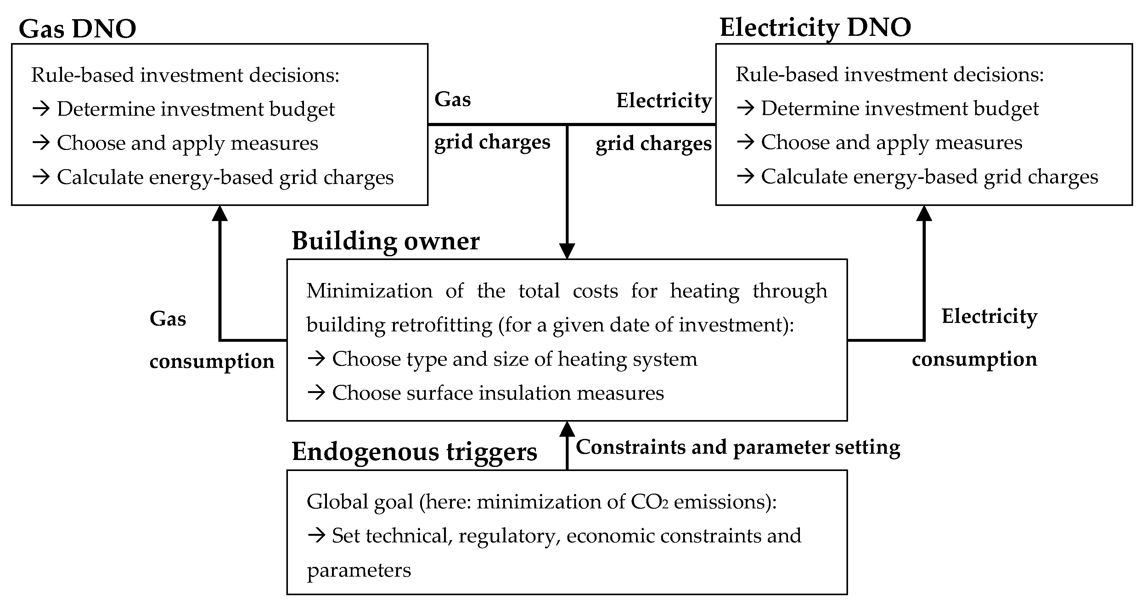
3.1. Research Approach

We postulate an interdependence between building owners’ and the electricity and gas network operators’ investments. Due to different triggers, gas-based heating systems are substituted, which leads to a decrease in demand and thus an increase in gas grid charges. The increase in electric heat pumps has a reducing effect on electricity grid charges, which further accelerates this development. A self-reinforcing mechanism starts, which can lead to a complete defection of the gas network. We address this issue with a multi-agent simulation (MAS), where the distributed autonomous and independent acting residential building agents interact with the natural gas and electricity grid, each of which is operated by a DNO agent (Figure 1).
The buildings, and respectively their owners (BOs), are represented by a mixed integer linear program (MILP). The BOs’ objective is to minimize the life-cycle costs of building retrofit measures focusing on space heating as well as drinking hot water generation and considering investment and operational expenditures. The degrees of freedom are the size and type of the heating system or the solar thermal system and the surface insulation thickness.
The gas and the electricity network operators act independently, represented by a rule-based model: Renewal, reinforcement, and closure measures are chosen considering the investment budget, which is determined by the strategy of each DNO and constrained by the regulatory environment; load and pipe flows simulations are carried out to ensure a supply within technical limits; total yearly grid costs are summed up in a cash flow calculation and passed on to customers in the form of energy-based grid charges.

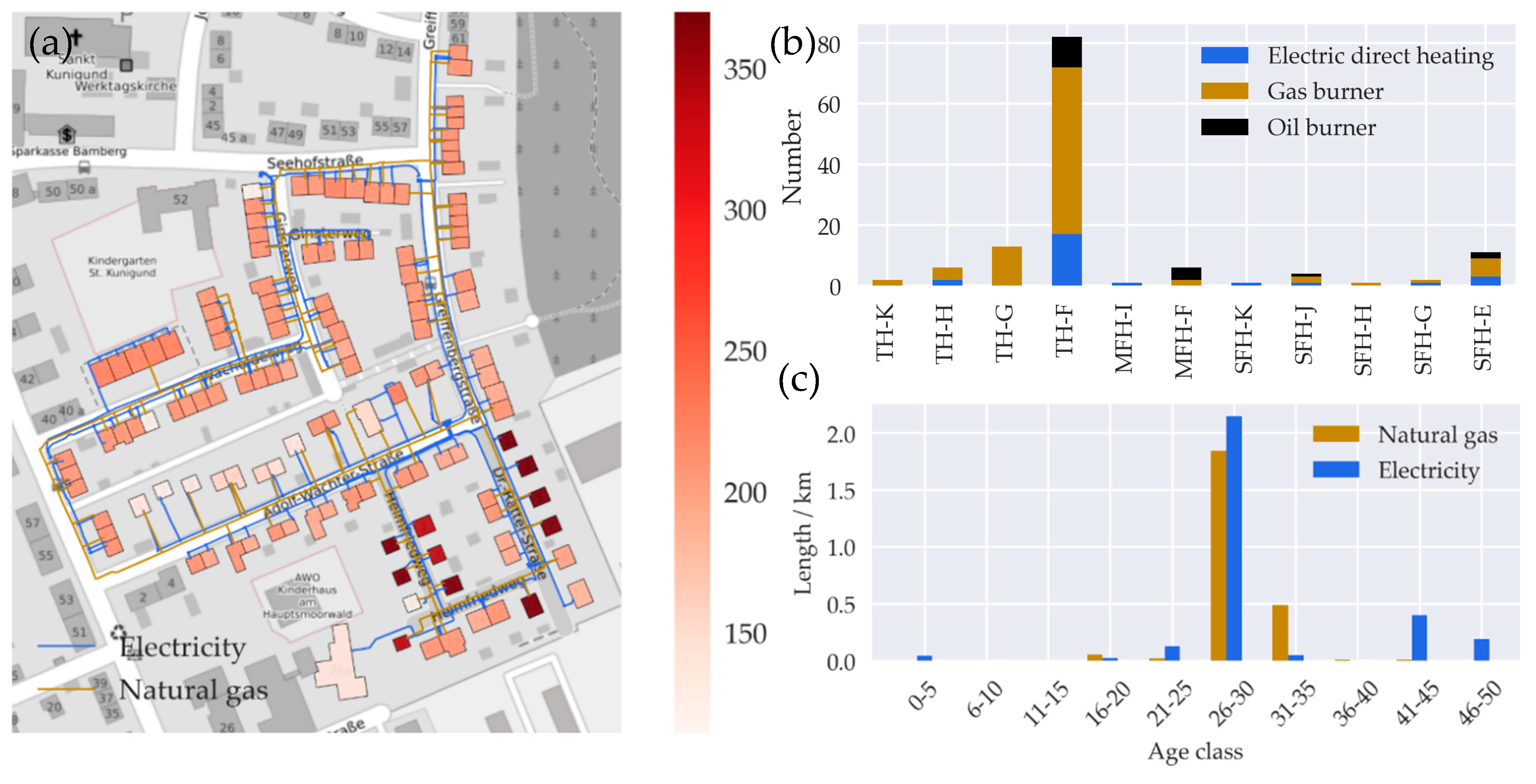
3.2. Grid and Building Data and Software Tools

We base our investigation on real data of a residential area in the southern German city of Bamberg (Figure 2a). The 129 buildings are supplied via a 2987 meter-long low voltage grid with an average age of 29.3 years, and a 2432 meter-long low-pressure grid with an average age of 29.5 years (Figure 2c). Both grids are connected to the upstream medium voltage, i.e., the pressure grid. The corresponding connection points are the medium to low voltage (MV/LV) transformer and the medium to low (MP/LP) pressure regulator station, which are modeled by a feeder. The buildings are assigned to reference buildings (according to the institute of housing and environment (IWU) in the TABULA project (typology approach for building stock energy assessment)) based on their energy consumption, floor space, and type [61,62]. The average reference area of the buildings is 137 m² and the average specific heating demand is 208 kWh/(m²·a), with 67% gas-bound, 20% electric and 13% oil-bound heating systems (Figure 2b). The heating circuit temperatures and building equipment are mapped to the buildings based on their renovation status and their initial heating system based on Open Street Maps [63] and census data (spatial resolution: 100 × 100 m) [64].
The area is supplied by the city’s DNO, which is responsible for the electricity as well as the gas supply. The electricity DNO has a revenue cap of approx. 20 M€ and the gas DNO has a revenue cap of approx. 10 M€. Table 2 shows the percentage distribution of the cost components of the revenue caps. Grid data were provided by the DNO: Line and asset data are from the geo-information system and the internal asset database; georeferenced metering information (energy consumption) of individual grid users is from the energy data management system; and the cost components of each revenue cap are from the cost allocation sheet. All data were recorded in 2018 for the financial year 2017. The software-based models were created on a Python basis, using pandapower [65] for the load flow calculations in the low voltage grid, Mesa [66] for the multi-agent simulation, NetWorkX [67] for the graph analysis, and Pyomo [68,69] together with the commercial solvers CLPEX [70] and Gurobi [71] for the optimization. For the pressure loss calculations, we have used the commercial software STANET [72].

3.3. Building Retrofit Optimization Model

The objective of the model is to minimize total expenditure c 𝒿 B (Equation (1)). This includes the capital expenditures for a change of the heating system c 𝒿 BES , the improvement of the building envelope c 𝒿 BE , the operational expenditures for maintenance c 𝒿 M , and energy procurement c 𝒿 EN . The expenditures are calculated for the expected technical lifetime of the heating system T based on annual time steps t for each building 𝒿 of the area 𝒥. For a list of the acronyms used, see Table A2 in Appendix B.1.
min c 𝒿 B = c 𝒿 BE + c 𝒿 BES + c 𝒿 EN + c 𝒿 M
For this purpose, the optimizer can choose the surface insulation thickness 𝓭 out of the available thicknesses D , represented by the decision variable b 𝓭 , 𝒿 B E and the heating system 𝓴 out of the available systems K , represented by b 𝓴 , 𝒿 B E S . A solar thermal plant 𝓼 out of the available systems S can be added, represented by b 𝓼 , 𝒿 S T E .
We model the building surface in a single-zone model, calculate the design-relevant heat load S 𝓭 , 𝒿 BE based on DIN EN 12831 (German and European harmonized standard) [73], evaluate insulation measures following [74], and choose parameters based on [37,75,76,77,78,79,80,81]; see Supplements A.1, A.2, and A.4. The investment expenditures for the building envelope (BE) c 𝒿 BE depend on the insulation thickness of the building surface area A 𝒿 E and the equivalent insulation thickness D D   (Equation (2)). The optimizer decides whether to retrofit the building surface and can choose thicknesses between 0 and 30 cm. The cost parameters C 𝒿 BEvar and C 𝒿 BEfix are calculated individually for every building based on the area ratios of the individual surface parts 𝓅 and costs [75]: roof, facade, windows, floor, and door.
c 𝒿 BE = 𝒹 D A 𝒿 E ( ( C 𝒿 BEvar D 𝓭 D ) + C 𝒿 BEfix ) b 𝓭 , 𝒿 B E ; w i t h   A 𝒿 E = 𝓅 𝓅 𝒿 A 𝒿 , 𝓅 EP ; C 𝒿 BEfix = 𝓅 𝓅 ( C 𝒿 , 𝓅 BEfix A 𝒿 , 𝓅 EP A 𝒿 E ) ;   C 𝒿 BEvar = 𝓅 𝓅 ( C 𝒿 , 𝓅 BEvar A 𝒿 , 𝓅 EP A 𝒿 E )
The investment expenditures c 𝒿 BES for the building energy system (BES) are dependent on the building heat load S 𝓭 , 𝒿 BE , which includes transmission and ventilation losses. S 𝓭 , 𝒿 BE is a function of the building insulation thickness D D as well as the initial building and usage properties. C 𝓴 BESvar represents the variable, C 𝓴 ,   𝒿 BESfix is the fixed parts of the expenditures, and C 𝓼   STEvar as well as C 𝓼 , 𝒿   STEfix are the expenditures of the solar thermal plant (STE) S 𝓼 , 𝒿   STE (Equation (3)). The solar thermal plant is modeled based on [62,82,83] and covers a part of the demand for drinking hot water S 𝒿 DHW , dependent on the choice of the heating system and the type of the solar thermal plant; see Supplement A.3. All cost components are calculated individually for each building in a preprocessing procedure based on the initial building equipment and the possible building equipment options (see Supplement A.5).
c 𝒿 BES = 𝓴 K ( ( 𝓭 D ( S 𝓭 , 𝒿 BE b 𝓭 , 𝒿 B E ) C 𝓴 BESvar ) + C 𝓴 ,   𝒿 BESfix ) b 𝓴 ,   𝒿 B E S + 𝓼 S ( ( S 𝓼 , 𝒿 STE C 𝓼   STEvar ) + C 𝓼 , 𝒿   STEfix ) b 𝓼 , 𝒿 S T E
The expenditures for energy procurement c 𝒿 EN are a function of the yearly energy demand (Equation (4)). They are calculated based on the heat load S 𝓭 , 𝒿 BE and the domestic hot water demand S 𝒿 DHW , which is reduced by the solar thermal plant S 𝓼 , 𝒿   STE and S 𝒿 S . S 𝒿 S represents parts of the heat load that are not affected by the renovation measures in our model: heat distribution losses, auxiliary energy, radiation losses, and internal wins. The final energy demand is determined in consideration of the yearly usage hours T 𝒿 N and the plant expenditure figure of the heating system E 𝓴 BES . The energy price C c , 𝓉 = 𝓉 I n v e s t EC is calculated based on the year of investment 𝓉 = 𝓉 I n v e s t and discounted with the present-value factor PF. We consider the energy procurement price C c , 𝓉 Proc , tax C c , 𝓉 Tax , and grid charges c c , 𝓉 = 𝓉 I n v e s t GC . The charges represent the dual variable, making the building owner investment decision interrelated to the one of the DNOs for grid-bound systems.
c 𝒿 EN = 𝓴 K ( ( ( 𝓭 D ( S 𝓭 , 𝒿 BE b 𝓭 , 𝒿 B E ) +   S 𝒿 S ) b k ,   𝒿 B E S + 𝓼 S ( S 𝒿 DHW ( S 𝓼 , 𝒿   STE b 𝓼 , 𝒿 S T E ) ) b 𝓴 , 𝒿 B E S ) T 𝒿 N E 𝓴 BES c C ( B c , 𝓉 EC C c , 𝓉 = 𝓉 I n v e s t EC PF ) ) w i t h   C c , 𝓉 = 𝓉 I n v e s 𝓉 EC = { C c , 𝓉 = 𝓉 I n v e s 𝓉 Proc + C c , 𝓉 = 𝓉 I n v e s 𝓉 Tax + c c , 𝓉 = 𝓉 I n v e s 𝓉 GC , f o r   c = electricity c = gas C c , 𝓉 = 𝓉 I n v e s 𝓉 Proc + C c , 𝓉 = 𝓉 I n v e s 𝓉 Tax , f o r   c = pellet c = oil
The yearly expenditures for maintenance c 𝒿 M are influenced by the heating system and solar thermal plant type and size, modeled via a fixed yearly rate M 𝓴 BES . It dependent on the investment expenditure of the heating system [76] and is discounted via the present value factor PF (Equation (5)).
c 𝒿 M = 𝓴 K ( ( 𝓭 D ( S 𝓭 , 𝒿 BE b 𝓭 , 𝒿 B E ) C 𝓴 BESvar ) + C 𝓴 , 𝒿 BESfix ) b 𝓴 , 𝒿 B E S M 𝓴 BES PF + 𝓼 S ( ( S 𝓼 , 𝒿 STE C 𝓼   STEvar ) + C 𝓼 , 𝒿   STEfix ) M 𝓼 STE b 𝓼 , 𝒿 S T E PF
To linearize the nonlinear mixed integer program, we use an approach according to [84]. The decision variables are constrained so that one renovation measure of the heating system has to be performed. The construction of a solar thermal plant and the renovation of the building envelope are possible options. For the constraints used, see formulas A1–A7 in Appendix B.2.

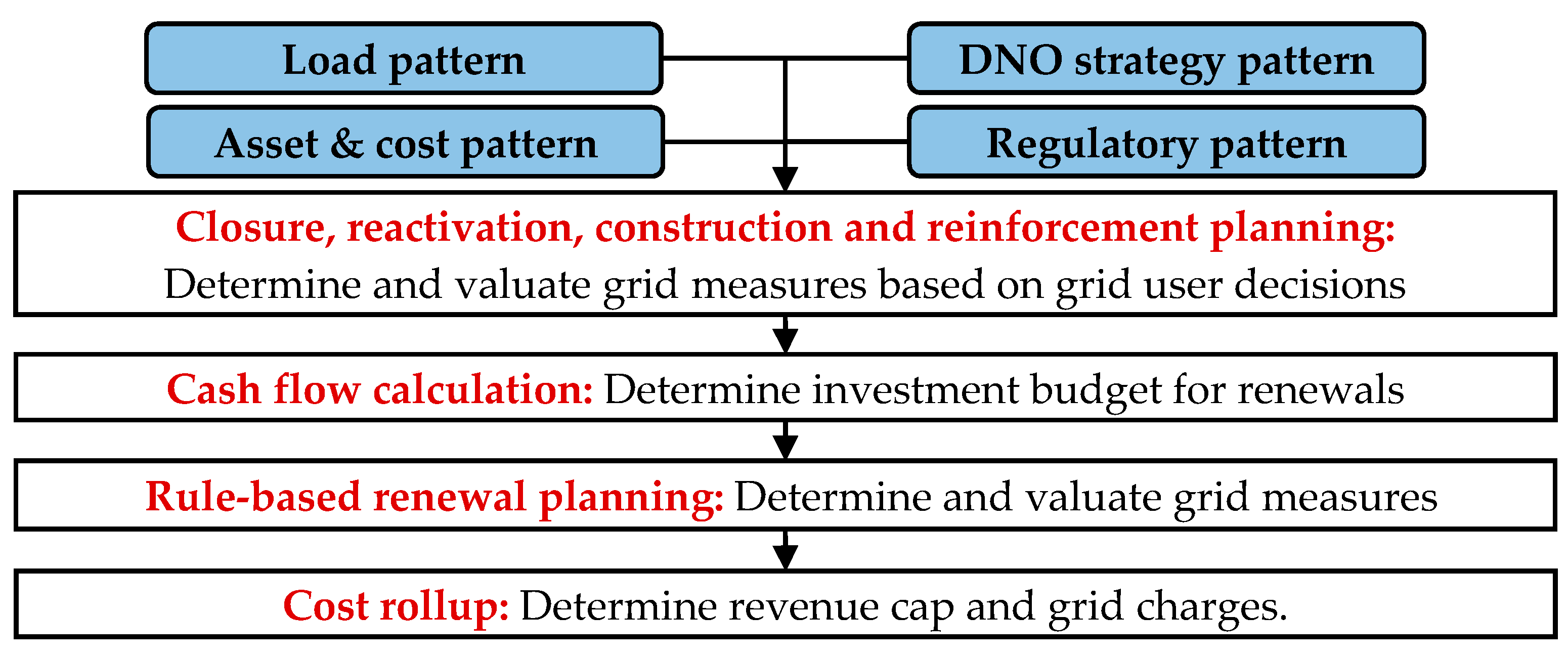
3.4. Distribution Network Operator Model

Within the multi-agent simulation the gas as well as the electricity DNO agent perform several steps (Figure 3).
First, the DNO reacts to the building owners’ decision by planning the grid closure, reactivation, construction, and reinforcement measures necessary for grid operation within technical boundaries. In the next step, the investment budget for renewal measures will be determined based on a cash flow calculation, considering its strategy and costs structure and the energy supplied, as well as the grid length and age. Individual measures are chosen with regard to an age-based renewal strategy [85]. In the last step, the revenue cap and resulting grid charges are determined (Figure 3). Load flow [65] or pressure loss calculations [72] are carried out to check technical limit values, whereby voltage drop and load are checked for electricity grid, and pressure and flow velocity for the gas grid.
The revenue cap is split into CAPEX and OPEX and passed on to the grid users in form of grid charges c c , 𝓉 GC (Equation (6)). These charges depend on the energy supplied for heating applications in the gas grid e c = Gas , 𝓉 Heating or electricity grid e c = electricity , 𝓉 Heating and other demands E c , 𝓉 AnyOther . Both the energy demand and the grid charges are the dual variables of the model [29]. For a list of the acronyms used in the DNO model, see Table A3 in Appendix C.1.
c ϵ T : α c , 𝓉 CAPEX + α c , 𝓉 OPEX c c , 𝓉 GC ( e c , 𝓉 Heating + E c , 𝓉 AnyOther ) = 0 ; with   α c , 𝓉 CAPEX = α c , 𝓉 EC + α c , 𝓉 BC + α c , 𝓉 Tax + α c , 𝓉 Depr ; α c , 𝓉 OPEX = α c , 𝓉 OC + α c , 𝓉 LC + α c , 𝓉 UpGC + α c , 𝓉 Cone
We show the calculation systematics of the individual cost components of CAPEX based on electricity lines (𝒸 = electricity). The approach can be transferred analogously to other grid assets of electricity and gas networks. For all lines in operation L , the return on equity (Equation (7)), the interests on borrowed capital (Equation (8)), and the trade tax (Equation (9)) are calculated based on the individual rest book value (factor) RBVF , 𝓉 , and the historical acquisition costs C I , as well as the equity Q EC or debt ratio Q BC , the corresponding interest rates R EC or R BC , or the trade tax rate R Tax . For lines in operation within the technical lifetime T TL , depreciations are calculated based on the initial line age T init and considered via C , 𝓉 Depr (Equation (10)). If a line is renewed or shut down before the end of its lifetime, the resulting special depreciation is excluded from the revenue cap [47].
α 𝓉 EC = R EC Q EC ϵ L C I RBVF , c
α 𝓉 BC = R BC Q BC ϵ L C I RBVF , 𝓉
α 𝓉 Tax = R Tax R EC Q EC ϵ L C I RBVF , 𝓉
α 𝓉 Depr = ϵ C , 𝓉 Depr ; w i t h   C , 𝓉 Depr ( 𝓉 ) = { L C I 1 T TL , f o r   t + T init < T TL 0 , f o r   t + T init T TL
For the determination of OPEX, we proceed as follows (𝒸 = electricity): The operating costs are modeled linearly dependent on the grid length based on C LRC (Equation (11)). Loss costs dependent on the loss factor F Loss (Equation (12)), upstream grid costs (Equation (13)), and concession fees (Equation (14)) are modeled based on the corresponding specific costs C LC , C UpGC , and C Conc , directly proportional to the dual variable e 𝓉 Heating and thus to the energy supplied.
α 𝓉 OC = C LRC ϵ L
α 𝓉 LC = ( C LC F Loss ) ( e 𝓉 Heating + E 𝓉 AnyOther )
α 𝓉 UpGC = C UpGC ( e 𝓉 Heating + E 𝓉 AnyOther )
α 𝓉 Conc = C Conc ( e 𝓉 Heating +   E 𝓉 AnyOther )
The DNO’s degree of freedom lies in the determination of grid measures. Thereby, we distinguish between (a) measures necessary for grid operation and (b) measures to maintain the grid value:
(a)
The grid length and energy supplied are predetermined by the building owners’ decisions in each year. As the DNO has to guarantee a non-discriminatory supply to all customers [46], measures have to be applied to fulfill the supply task within technical limits.
(b)
The DNO has to ensure a reliable and cost efficient supply [46]: We choose an age-related renewal strategy for the low voltage and the low pressure grid.
Once the measures necessary for network operation (a) have been carried out, all lines or pipes are sorted by age and renewed from old to young (b) until the investment budget is reached. The budget depends on the DNO strategy; see Figure A1 in Appendix C.2. The basic idea of all strategies is to keep the respective target on a constant level by reducing or increasing investments according to (b). Measures according to (a) reduce the investment budget, which, in extreme cases, leads to a change in the respective target figure (RC, GC, grid age). To avoid exotic age distributions, the asset age is limited to half and double the individual technical lifetime T TL [22].

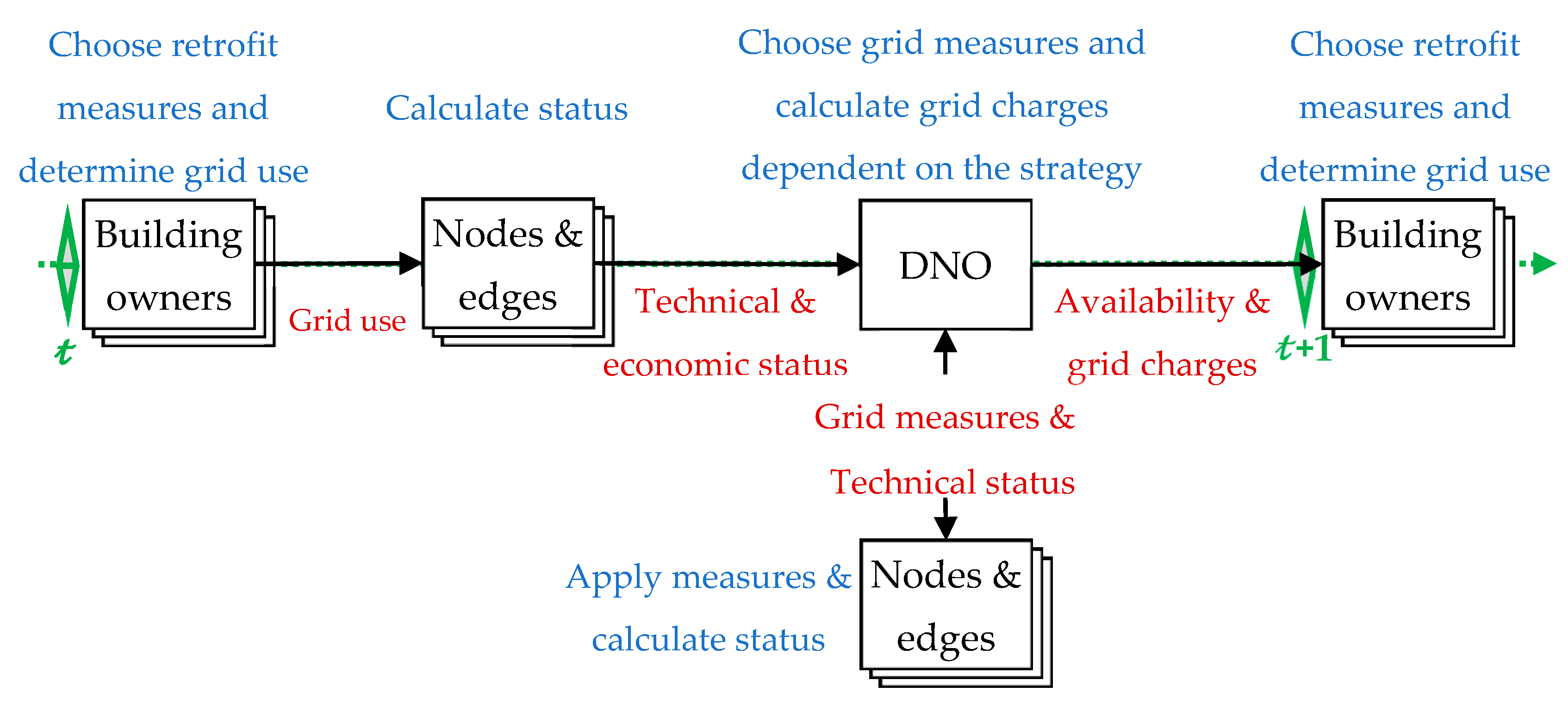
3.5. Multi-Agent Simulation

All buildings and respectively the owners and all assets of the gas and electricity grid are modeled as own agents. Technical and economic parameters are propagated to the DNO via a predefined hierarchy. Vice versa measures are delegated to the respective asset (see Supplements B.1 and B.2). The agent model determines how the individual grid agents are instantiated and initialized in a given electricity or gas distribution network and regulates the activation sequence of the agents as well as the communication between them. The agency is the total of all agents and includes all created grid agent instances, building agents, and the scheduler modeled with the Python package MESA [66]. Our agency implements the MESA model class and imports the MESA scheduler class. New grid agent objects that implement the MESA agent class are created via the agency class and added to the scheduler.
Table 3 shows the implemented agent types according to [86,87,88,89,90]. Each agent has a different level of complexity, which is reflected in their element-specific tasks in consideration of the individual design goals [60,91]. All agents, even the nodes, lines, and pipes of the grid are reactive. They are triggered by stimuli (input) from their environment and generate actions (output) [60]. For example, if a gas pipe does not receive a gas demand from its neighboring node (input), it triggers an event (output), indicating that it can be closed. The main benefit of this modeling approach is the decomposition and modularization of a complex and dynamic system or problem, in our context the interaction between grid assets and buildings [86]. Furthermore, it reduces the effort needed to expand or modify parts of the simulation system, e.g., change the individual agent specific design goals.
We have classified the MAS according to [92] and interpret the properties as follows (Table 4):
  • “Accessibility“ describes the ability of an agent to access all other agents of the network;
  • “Deterministic“ describes if the cause–effect relationship of actions of agents is known or not;
  • “Episodic” describes whether the simulation time steps are interrelated;
  • “Dynamic” describes the possibility of environmental changes beyond the control of an agent;
  • “Discrete” describes if there is a predetermined number of perceptions and actions.
The gas or electricity network is modeled as a graph in an undirected tree, in which the agents are arranged hierarchically [93]. This corresponds to a radial grid structure. All agents are executed once during a time step starting at the lowest element—the “Building owner”—and ending at the highest element—the "Network operator". Thus, the information is propagated from the bottom up, meaning that the network operator follows the investment decision of the building owner; see Figure 4.
The scheduling method follows a breadth first search (BFS) algorithm in the reverse direction [92]. Conventionally, the BFS traverses a graph from the top to the bottom layer after activating all nodes of a layer, where the algorithm expands in width until it terminates when all nodes have been visited. As we turn this mechanism around, our algorithm terminates after activating the DNO (see Supplement B.1).

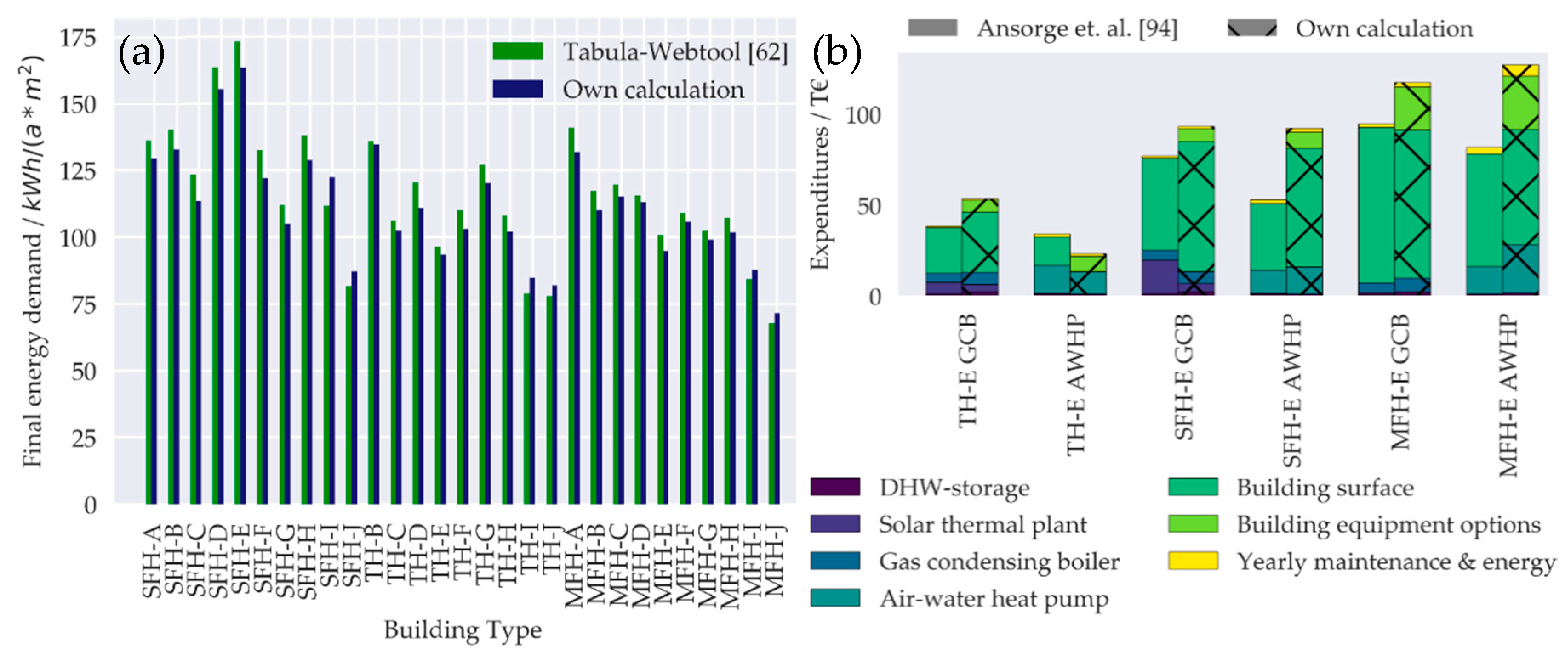
3.6. Validation of the Building Model

We validated our results for different building types—a single family (SFH), a terraced (TH), and a multi-family house (MFH), and age classes from approx. 1900–2009 (A–J) [61,62] within the literature. For the energy calculation we compared with [62] and for the cost calculation with [94]. Figure 5a shows the results of the yearly final energy demand normalized by the reference floor area (gas-based solution): For buildings of the age classes A–H, we underestimated the energy demand by 5% on average; for classes I–J, we overestimated by 6% on average. The differences are induced by internal and drinking hot water generation losses, which we modeled according to [95]. We assume that the energy calculation model and its parameterization is valid for the present study, as the deviations are below the level caused by individual user behavior in terms of room temperature and ventilation [96,97].
Figure 5b compares the expenditures of the three buildings types for a gas- and an electricity-bound solution (SFH-E, TH-E, MFH-E), which represent the majority of the building stock of case studies 4.2, 4.3, and 4.4. While the end energy demand of the six buildings after retrofitting is well matched (mean deviation: 5.8%), the cost calculation shows deviations between −5 and 40%, which is caused by the parameterization of the cost functions. We use parameters considering [75], where the authors analyzed costs of building and heating system retrofit measures for 1117 buildings in Germany and showed that there is a great variance in practice: The standard errors for thermal insulation systems depicts 6.9% for C 𝒿 BEfix and 15% for C 𝒿 BEvar in full costs (facade). Another reason for the deviations results from different assumptions regarding the reference floor and surface area of type buildings and the consideration of the initial building equipment options, rather the costs of retrofitting (e.g., gas grid connection, oil tank or heating circuit temperature). We modeled these equipment options by adjusting the parameters of the cost functions of the individual measures based on the individual initial building equipment options in preprocessing.

3.7. Conception of the Case Studies

3.7.1. Case Study 1: Sensitivities of Building Retrofit Decisions

In this case study, we faced the question of how electricity and natural gas grid charges influence the choice of building and heating retrofitting measures. For that reason, we analyzed the retrofit decisions of 609 different building and heating system configurations for a variation of electricity and gas prices. The results can be used to classify and compare our findings of the case studies (4.2, 4.3, and 4.4) with the literature.
We varied energy prices by +23% and −12% for electricity and +25% and +50% for gas from the initial point and combined them in nine price scenarios. The price changes correspond to a change of grid charges in the electricity sector of −50% and +100% and in the gas sector of +100% and +200%. These price change levels were used as the relationship between demand and grid costs is non-linear and the expected development differs between gas and electricity. The investigation was based on the German average prices for electricity—30.85 ct/kWh—and gas—6.34 ct/kWh—for a medium-sized residential building (energy consumption electricity: 3500 kWh/a, gas: 5556–55,554 kWh/a) [79].
We focused on residential buildings (SFH, TH, MFH) and summarized the building age classes: A–C are buildings constructed before the foundation of the Federal Republic of Germany in 1948; D–F are from before the first thermal insulation ordinance (1949–1978); G–H are according to Thermal Insulation Ordinances 1 and 2 (1979–1994); and I–J are according to Thermal Insulation Ordinance 3 and the First Energy Saving Ordinance (1995–2009) [61]. We considered the following heating systems: Electrical air-water (AWHP) and ground-water heat pump (GWHP), electric direct heating (EDH), gas (GCB) and oil (OCB) condensing boiler, pellet burner (PB) and solar thermal plants (STE), with the different heating system temperatures 90/70, 70/50, 55/45, and 35/28 (°C/°C), corresponding to the building equipment option. The whole building population (n = 609) was created by combining the properties building type (n = 3), age (n = 10), heating system (n = 6), and heating circuit temperature (n = 4), where technically impossible combinations were discarded.

3.7.2. Case Study 2: Analysis of Possible Triggers for a Decline in Gas Demand

In this case study, we answer the question of how building retrofit decisions and thus the natural gas and electricity grid costs are influenced by technological and regulatory triggers and are shaped by the individual initial building insulation status and heating type. Therefore, we distinguish eight types of triggers:
  • Taxation and levy systems: There is a wide spread of different taxation and levies and systems. We focused on CO2 pricing, as the German government has passed a law in 2019 that sets a CO2 price of 25 €/t in 2021, rising to 65 €/t by 2026 [98].
  • Grid charge models: In Germany, DNOs can reduce the electricity grid charges for interruptible grid users down to 20% of their regular value [99] (25% for the area under investigation).
  • Regulatory energy efficiency constraints: In Germany, regulatory constraints for new constructions and retrofittings are listed in the energy saving regulation [100], which will be tightened in the future [101]. We set the initial final energy demand and CO2 emissions as an upper bound in all simulations. Additionally, two scenarios were modeled, where we tightened the limit and set the primary target equal to the useful energy demand, calculated based on [100]:
    In simulation 3, 100% of the buildings have to perform a surface insulation measure and change their heating system to obtain the target.
    For simulations 8–10, we oblige only 66% of buildings to retrofit their envelope and heating system. 34% can freely choose the kind of measure to reach the efficiency target of [100]. This represents a surface renovation ratio of approx. 2%, corresponding to a technical lifetime of the surface of 50 years often used in literature [32].
  • State market incentive and subsidy programs: We consider the situation in Germany: For building envelope renovations, there is a state subsidy program, which on average subsidizes about 30% of investment expenditures [102]. For heat pumps, there is a market incentive program with an average subsidy rate of 40% [103].
  • Technological development: The efficiency of heat pumps is highly dependent on the coefficient of performance (COP), which is predicted to increase by about 25% in the next decade [104].
  • Decentralized energy generation: In recent years, heat pumps have increasingly been combined with photovoltaic plants and battery storage systems. We do not examine PV-battery systems in our analysis, as we focus on the effects on gas grids.
  • Initial building insulation status, heating type and date of investment: The initial building age class and heating system largely determines the date of investment and the choice of the renovation measure. As the age and the types of heating systems and buildings are heavily weighted in our dataset, we analyze scenarios with a variation (100 seeds) of the date of investment (I), the initial building age class (B), and the initial heating system (H). For that reason, we reconfigure the initial gas and electricity grid when varying the initial heating systems.
First, we analyze the influence of each of these triggers in simulations 1–6 (see Table 5, marked in grey). Second, we combine triggers, generating two sensitive but opposing scenarios with a high probability of occurrence for Germany: Simulation 7 induces a high proportion of gas-based solutions in the future system, while simulation 8 induces increased substitution of gas-based heating by other systems. Third, we evaluate the influence of a variation of initial building age classes (B) and heating system types (H) of the building stock in simulations 9–11 (marked in blue). These results are compared with simulation 8, since the same combination of triggers is in use. We vary the date of investment (I) for each building in 100 seeds in all simulations. Every building performs one retrofit during the planning horizon from 2020 to 2050, which corresponds to a lifetime of the heating systems of about 31 years; see Supplements C.1 and C.2 for the parameterization.
In the case studies in 4.3. and 4.4, we set the triggers corresponding to “Combination 2” (simulation: 8) because of:
  • Objective of the analysis: We focused on the evaluation of building owners’ and electricity and gas DNO’s strategies in transformation paths with a decreasing gas demand.
  • Probability of occurrence: In simulation 8, we have chosen each trigger corresponding to the situation in Germany, as there will be CO2 pricing in the future. There are subsidization programs, reduced electrical grid charges, and energy efficiency constraints.

3.7.3. Case Study 3: Interdependencies between the DNO’s Grid Charge Setting and Building Retrofit Decisions in Face of Decreasing Gas Demand

In this analysis, we address the question of how interdependencies between the DNO’s investment decisions and building owners’ retrofit decisions are shaped in scenarios with a decreasing gas demand. For that reason, we interrupt the communication of grid charges from DNO to the building owners during the multi-agent simulation, so that building owners decide based on the initial grid charges c c , 𝓉 G C = c c , 𝓉 = 0 G C . The results are compared with those of the simulation in which the building owners decide based on the grid charges of the year of building renovation c c , 𝓉 G C = c c , 𝓉 = 𝓉 I n v e s t G C ; see Table 6.
We focus on the situation in the gas sector, where we consider the two dual variables, analyzing their development during the planning horizon: The grid charges as a measurement of the sensitivity of grid costs to the given supply task during the transformation path, and the yearly gas demand as measurement for the sensitivity of building retrofit decisions to the costs of grid operation. Measuring the feedback effects between the building owners as well as the electricity and gas DNO allows us to answer the question whether grid costs are a trigger element that could accelerate the decline in gas demand and influence the technology transformation path of heating systems.

3.7.4. Case Study 4: The Influence of DNO Strategy Patterns on Grid Economy in the Face of Decreasing Gas Demand

In this study, we answer the question of how a change in the investment strategy of the gas DNO influences the following: The choice of building retrofit measures (measured by gas demand), the gas grid costs (measured by grid charges), and the profitability of the gas grid (measured by the revenue cap, grid length and age) in scenarios with a decrease in gas demand. For that reason, we compare three main strategies, whereby the DNO tries to keep grid charges (SGC), grid value (SGV), or the revenue cap (SRC) on a stable level during the planning horizon (see Table 1 and Appendix C.2).
We focus on the situation in the gas sector and set the triggers according to “Combination 2”. In simulations 8gc, 8gv, and 8rc the date of investment (I) of the buildings are varied and compared to simulations 10gc, 10gv, and 10rc, where the initial building age types and heating system types (I, B, H) are varied (Table 7). The results can be used to determine the effects of differently shaped regulatory systems on the DNO business model and the efficiency and quality of the gas supply.

3.8. Limits, Transferability, and Representativity of the Analysis

In order to guarantee transferability of the results, we used IWU-type buildings [61,62] in all case studies. We varied the date of investment (I), the initial building age classes (B), and the heating system (I) probabilistically in 100 seeds, which constitutes a representative sample size for the analysis in case studies 4.2, 4.3, and 4.4. For that reason, we limited the solution space for the building stock: The date of investment between 2020 and 2050 (n = 31); the building age classes between 1958 and 2015 (classes E–K, n = 7), and the possible initial heating systems to EDH, GCB, OCB, PB and AWHP (n = 5), each combined with the corresponding technical building equipment. Taking into account the number of buildings in the area (n = 129), this resulted in a number of possible combinations (population size) of 3999 for simulations (I), 27,993 for simulations (I, B) and 139,965 for simulations (I, B, H). For simulations (I), we estimated a representative sample size of about 94 seeds (margin of error = 0.1, standard deviation = 0.5, confidence level = 95%, population size = 3999).
The assumptions for the costs within the building investment model represent a medium case compared to the literature [75]. For the following reasons, the DNO model for gas and electricity underestimates the cost base compared to reality:
  • The grid charges for upstream grid levels ( α UpGCG ) are assumed to be constant during the planning horizon in both the electricity and gas sectors. In reality, these charges would also change with the demand.
  • The operational costs for the electricity and gas grid are formulated as linearly dependent on the grid length and independent on grid age. As they include components such as personnel costs and rents for buildings, they are in reality stepped fixed costs related to the grid length, which follow a change of the grid length delayed [22].
  • Costs for line closure measures of house connections in the gas grid are currently valued at 0 € per measure, as they can currently be allocated to the customer.

4. Results and Discussion

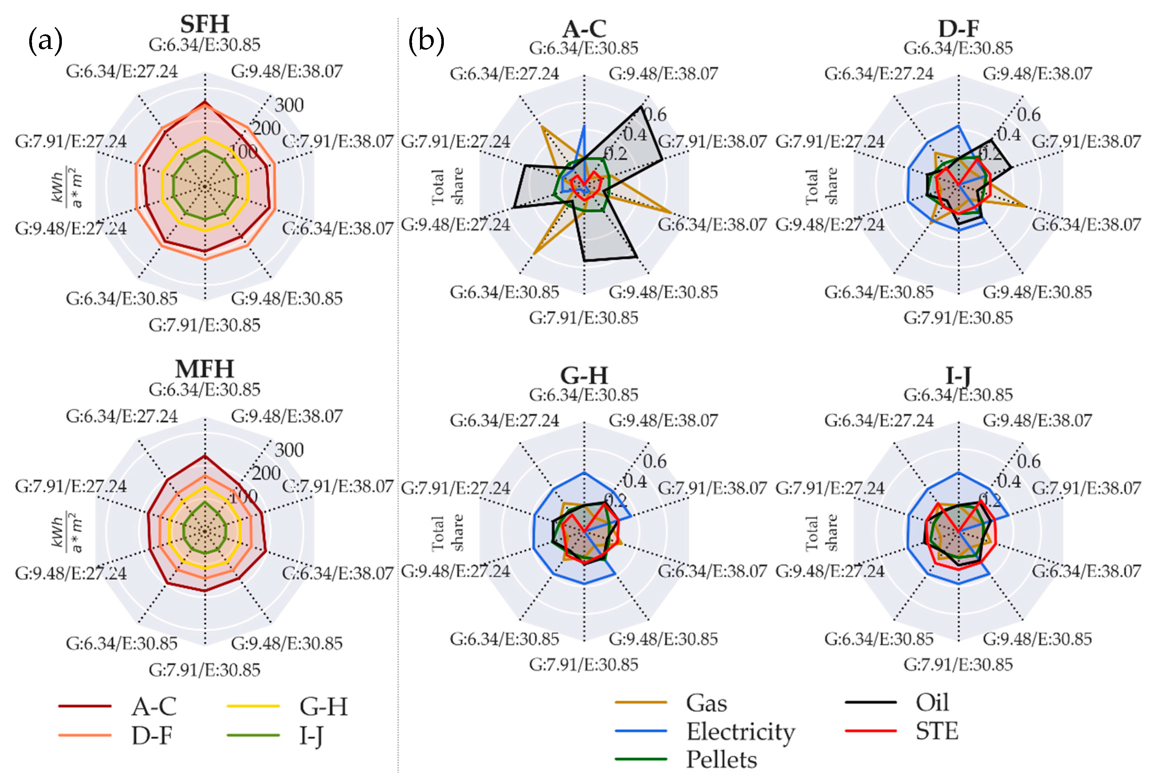
4.1. Case Study 1: Sensitivities of Building Retrofit Decisions

The results of the analysis of building retrofit decisions for the 609 type buildings in ten price scenarios are expressed as shares of the total sample (Figure 6b) or mean values of a part of the sample (Figure 6a). Figure 6a shows the specific final energy demand for single and multi-family buildings: When electricity and gas energy procurement expenses are high, insulation measures are increasingly chosen (20% of the buildings for G:9.48/E:38.07; 8.3% for G:6.34/E:27.24), primarily for older buildings (71% are applied in age classes A–C for G:9.48/E:38.07). Since insulation measures are expensive compared to other energy efficiency measures, they are chosen by only a small proportion of buildings when energy prices are high. Therefore, in reality they are mostly applied at the end of the technical life of the respective part of the building envelope [32].
Condensing boilers are increasingly being chosen in buildings of age classes A–C and D–F, where decisions are sensitive to energy price variations (Figure 6b): With a rising gas price they are substituted by oil-based systems or supplemented with solar thermal plants. Current regulations inhibit this trend in Germany [105]. Due to their high initial energy efficiency, heat pumps are becoming more attractive for G–H and I–J class buildings, often supported with solar thermal energy when electricity prices are high. The attractiveness of heat pumps depends strongly on the parameterization of the annual COP: We use the specifications of the Federal Office for Export Control for the market incentive program in Germany [106] and adapt them for different heating circuit temperatures [107]. Lowering the heating circuit temperature increases the efficiency of heat pumps, but is associated with costs, so it is not often chosen (e.g., 15% of the buildings for G:6.34/E:27.24).
The results imply that fluctuations in energy prices influence the investment decision for heating systems and surface renovations depending on the building age: With rising electricity and gas prices, insulation measures and solar thermal systems are increasingly chosen. Gas burners are more sensitive to energy price fluctuations than electric heat pumps because of their lower efficiency and their low investment compared to operational expenses. The attractiveness of electrical heat pumps increases with a rising building energy efficiency and annual COP. Conclusions can be drawn for the building stock of case studies 4.2, 4.3, and 4.4: Gas and oil condensing boilers in combination with solar thermal systems are increasingly being installed (77% of the buildings belong to building age class D–F, 17% to G–H, and 6% are younger, with 80% being terraced houses, 15% single family houses, and 5% multi-family houses).

4.2. Case Study 2: Analysis of Possible Triggers for a Decline in Gas Demand

We split the analysis of the eight trigger scenarios and the building type variations into three subsections: The building retrofit decision, the resulting energy demand, and the grid costs.

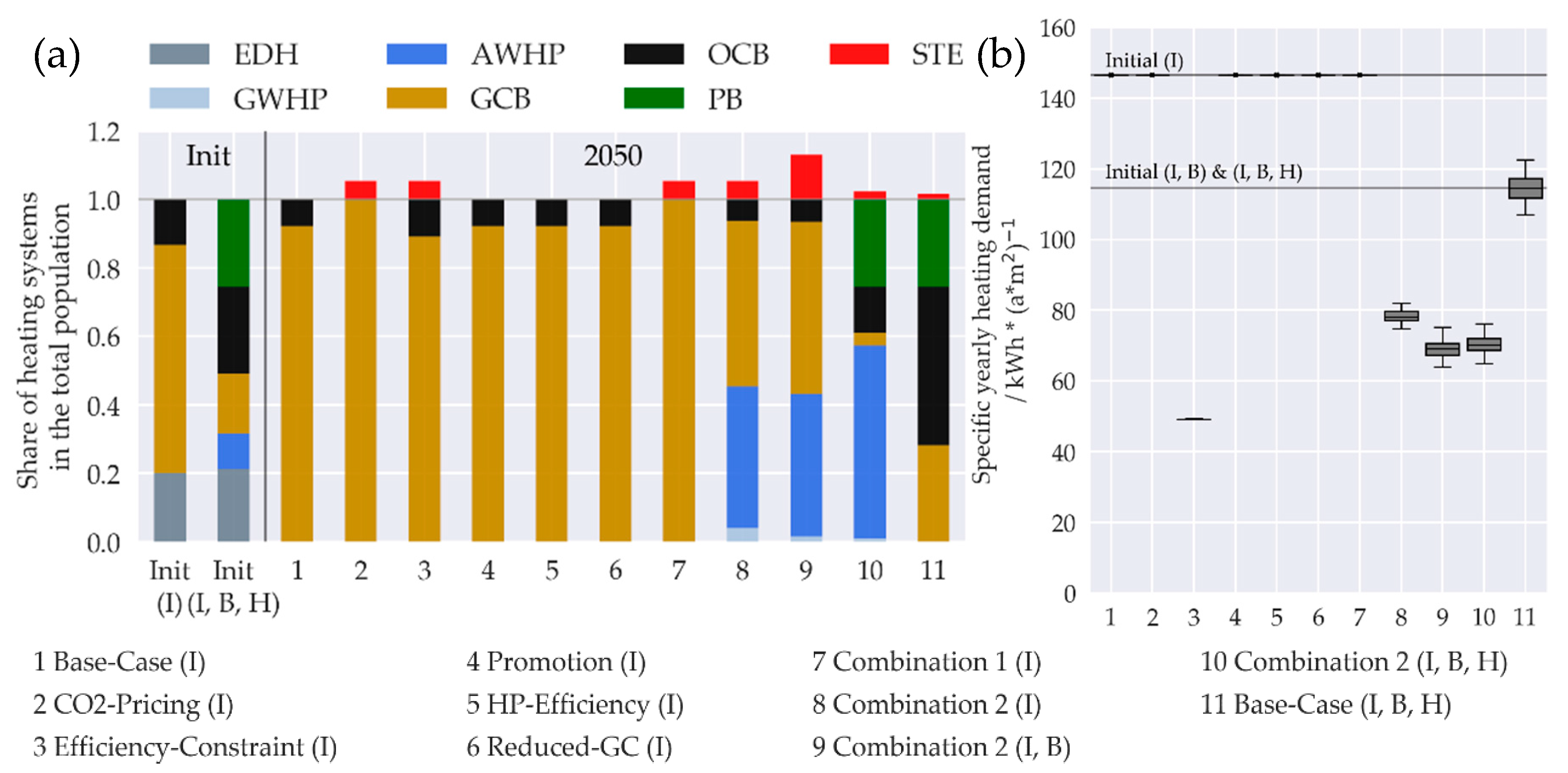
4.2.1. Investment Decisions of Building Owners

The results regarding the insulation measures (Figure 7b) support the findings from 4.1: The optimizer does not select an insulation measure if the choice of the measure type is not constrained and the energy saving constraints could only be achieved by a switch of the heating system (simulations 1, 2, 4–7). In this case, heat pumps come into play and substitute surface insulation measures (compare simulations 3 and 8). To generate scenarios with a real surface renovation rate, it must be constrained (simulations 3, 8–11).
Figure 7a shows that inefficient electrical direct heating is mostly substituted by gas condensing boilers (simulations 1–7). Due to the high initial connection rate to the gas grid (approx. 85%), the grid charges and with that the operational expenditures of gas-based heating are comparatively low. As gas grid connections are available in many buildings, the investment expenditures are also low for gas burners. With a drop of initially installed gas-based solutions, their usage is significantly reduced in target systems; compare simulation 8 and 10. A reduction of the heating circuit temperature, which is necessary for most buildings in the investigated area when switching to an electrical heat pump, is associated with higher costs compared to the solutions based on burners. The results for “Combination 2” hardly differ with a variation of building age class (simulations 8 and 9).

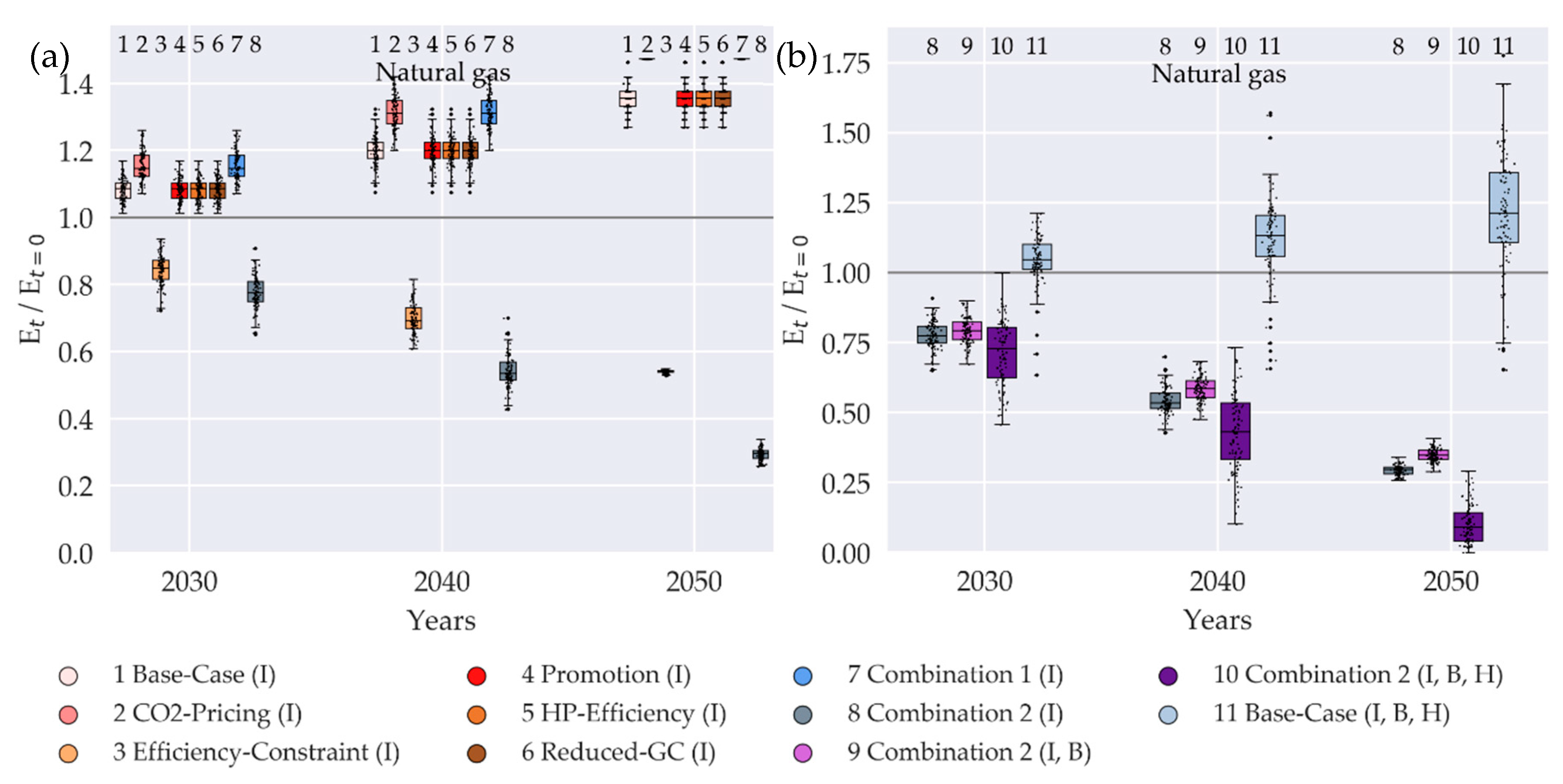
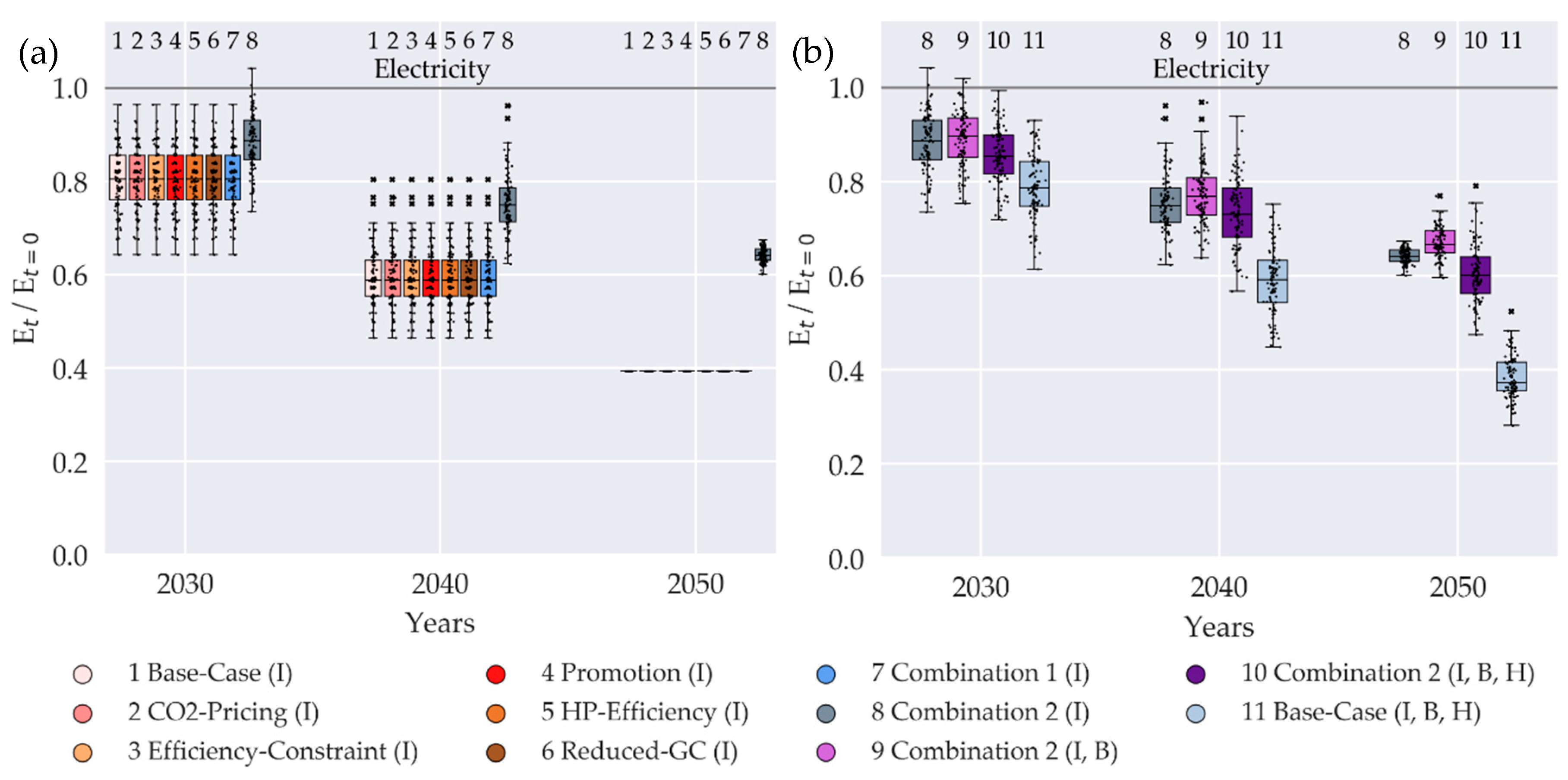
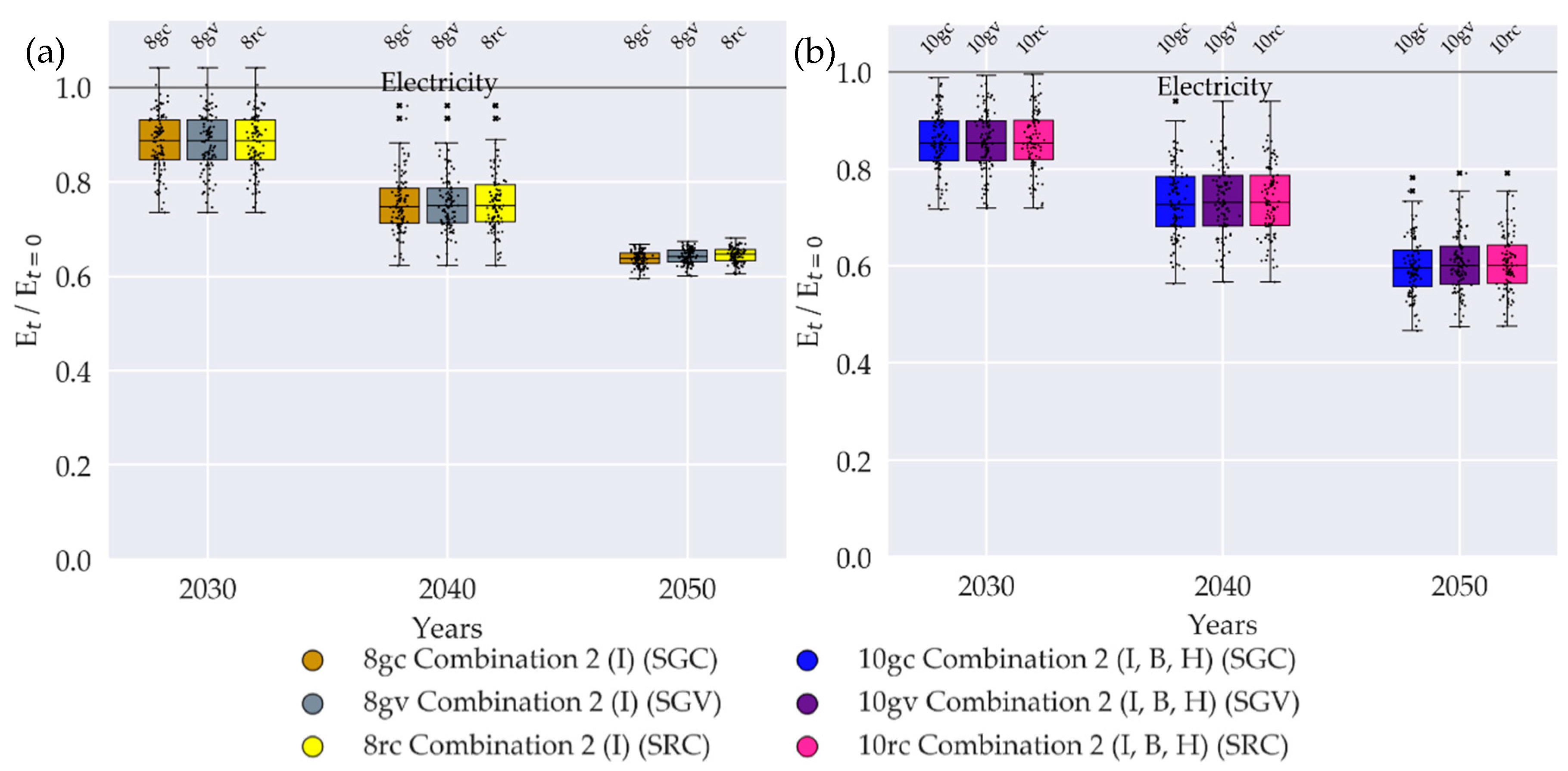
4.2.2. Resulting Gas and Electricity Demand

Figure 8 illustrates the transformation path of the natural gas demand for the projected years: 8a for different triggers (1–6) and their combinations (7–8), 8b for the variation of building age and heating types. In this area, gas is only used for heating applications; therefore a substitution of gas burners directly induces an increase (1, 2, 4–7) or decrease (8) in demand. Although in simulation 3 in 2050 approx. 90% of the heating systems are gas-based, we see a drop of about 55% in demand, which is induced only by surface insulation measures and solar thermal plants (Figure 7b). A comparison of simulations 8–10 shows that the initial building age and heating system configuration have a significant influence on the future supply task. A lower initial house connection rate in the gas grid increases the risk of a complete gas grid defection. While in simulation 8, the initial gas grid connection rate is 85%, in simulation 10, it depicts on average 20%. This causes higher initial grid charges and an increase of the specific investment expenditures for gas condensing boilers, which reduces their attractiveness in simulation 10. This effect can also be seen when comparing the “Base-Case” scenarios (simulation 1, 11). With a decreasing gas grid connection rate, the development of gas grid charges is therefore significantly more sensitive to endogenous economic, regulatory, and technical triggers. When looking at the electricity demand, another picture can be drawn, since the heating applications cover only a part of the supply task. For that reason, the substitution of electric direct heating systems causes a decrease of 35–60% from 2020 to 2050; see Figure A2 in Appendix D.1.

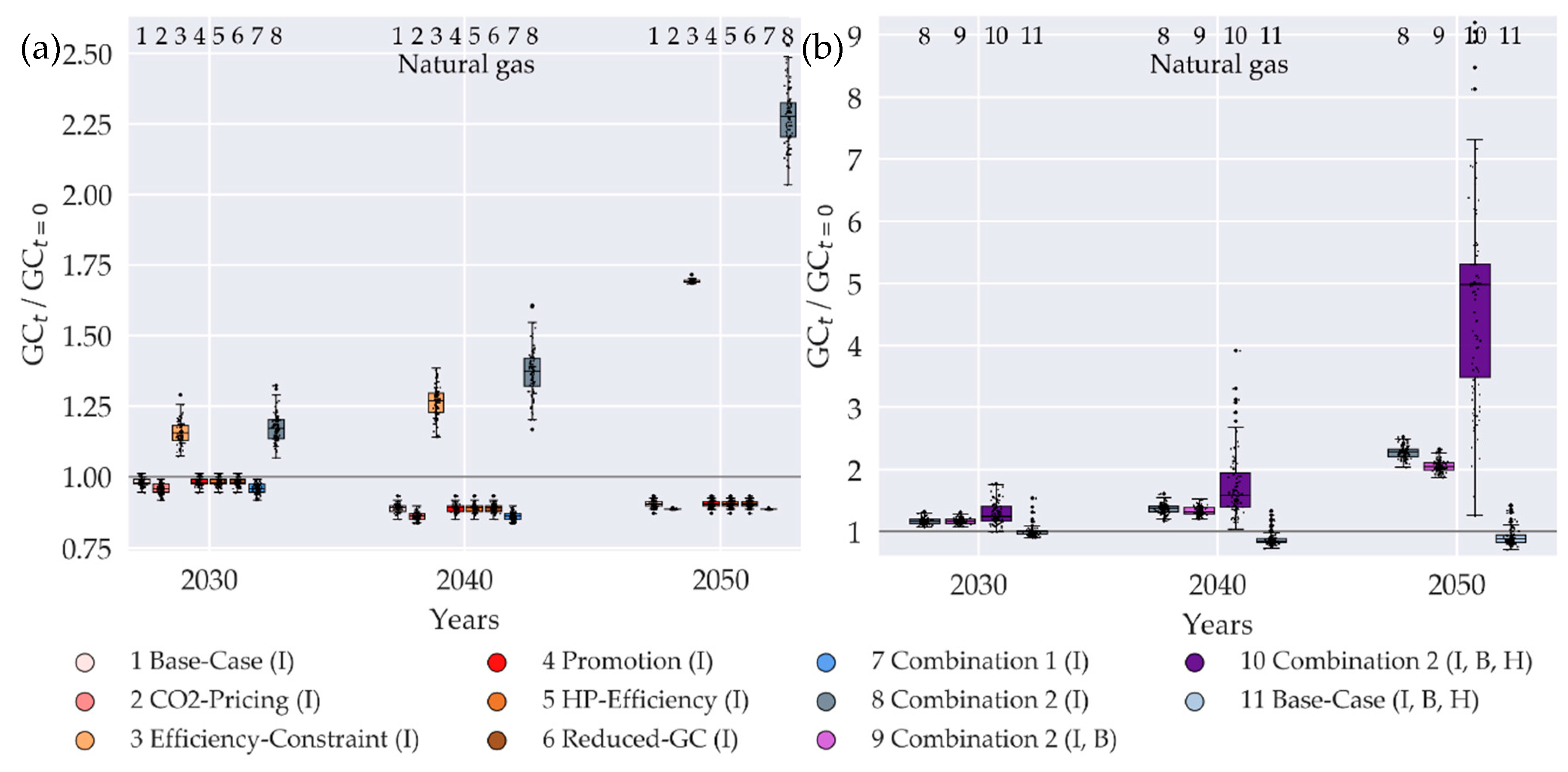
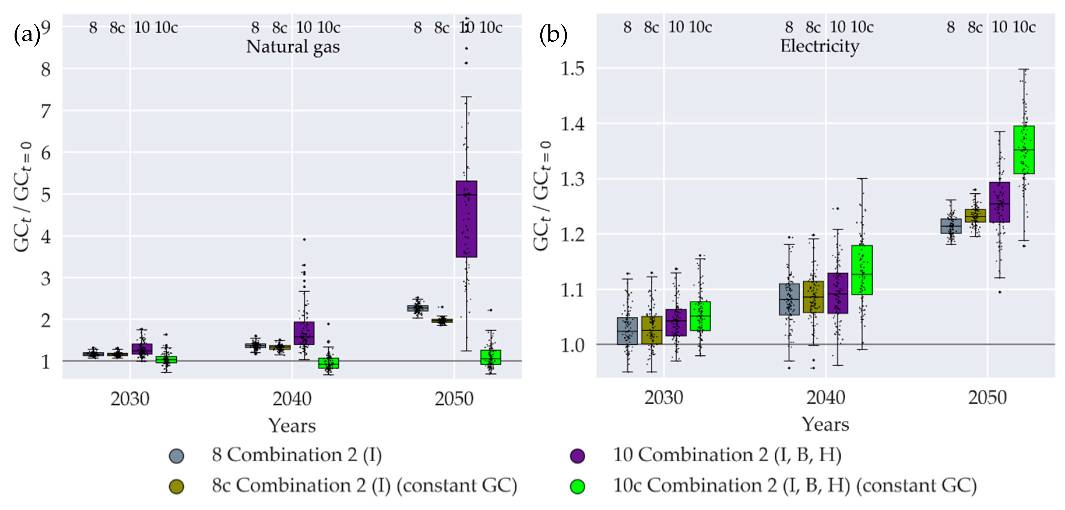
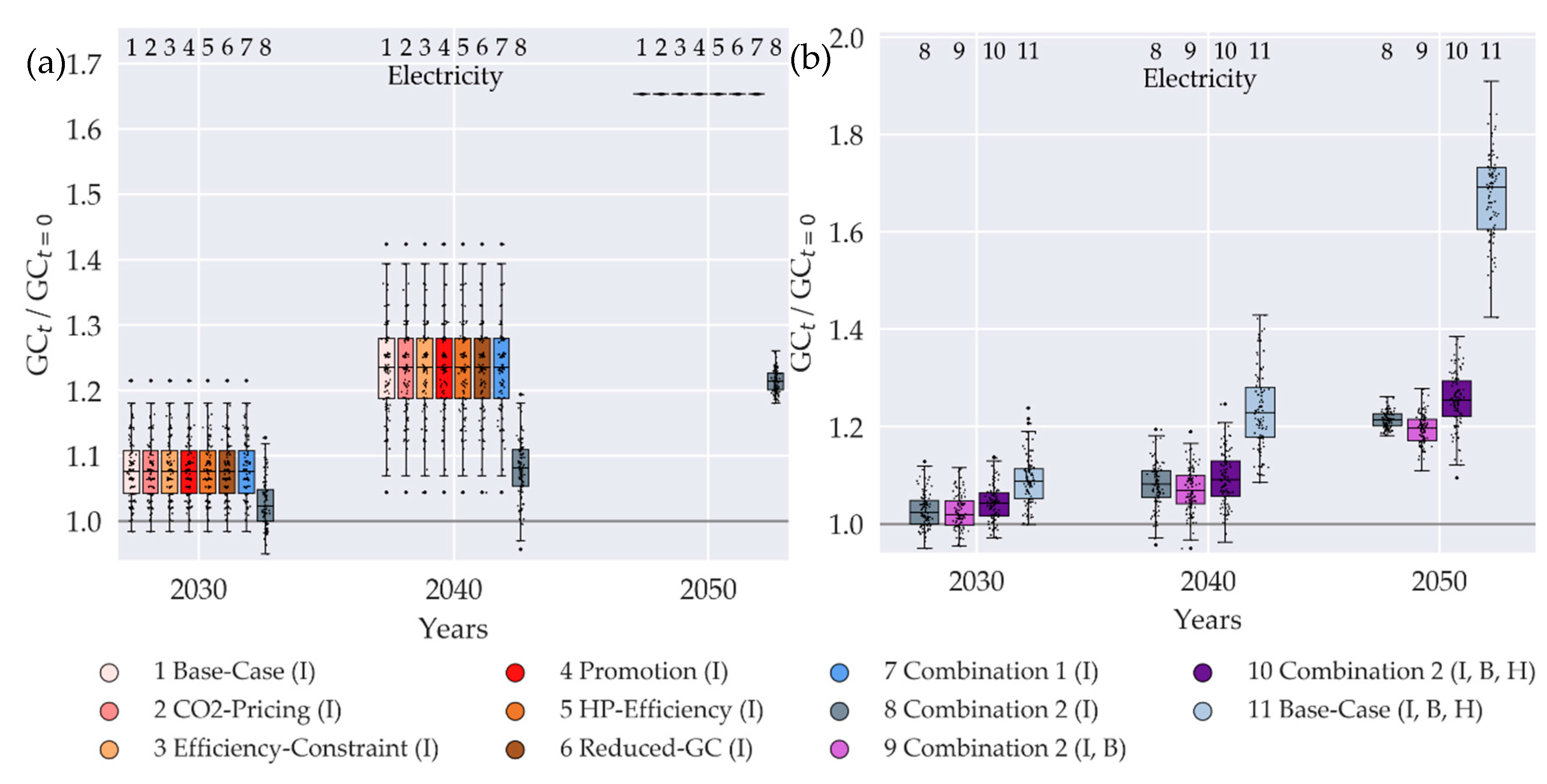
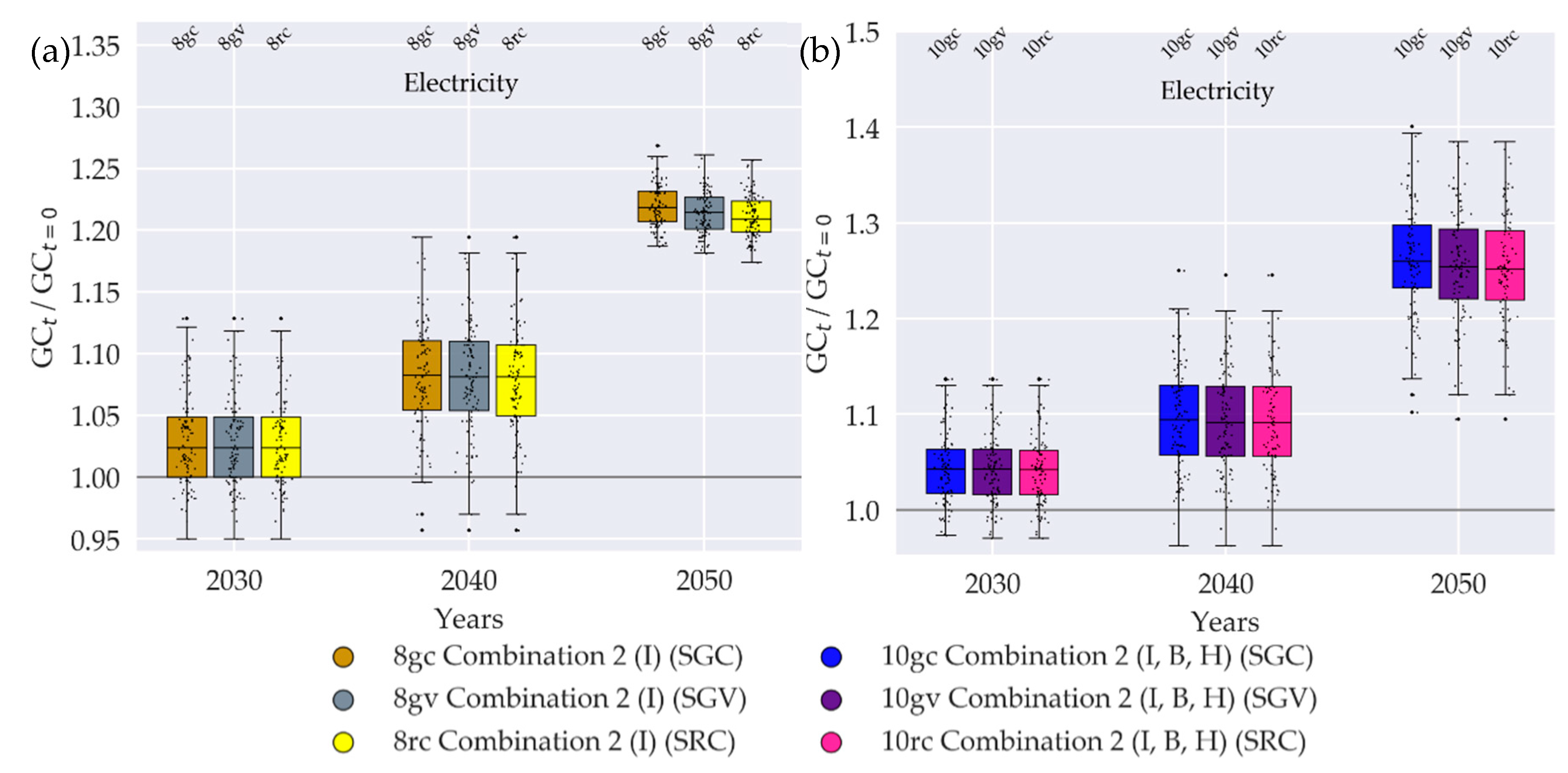
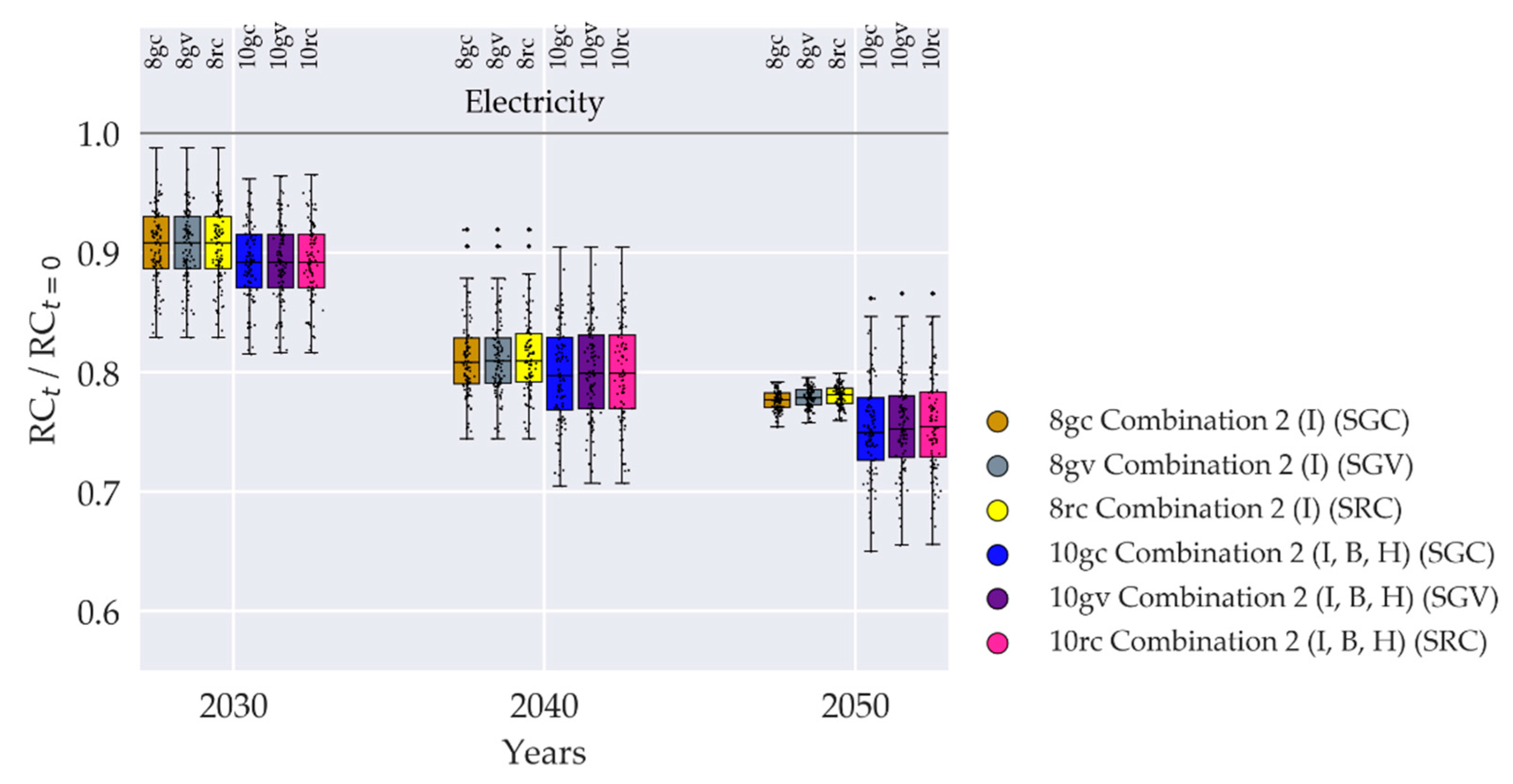
4.2.3. Impact on the Gas and Electricity Grid Charges

As the gas demand rises, the grid charges fall (1, 2, 4–7). As the demand falls, the effect reverses (3, 8), but is more pronounced (Figure 9a) due to the non-linear relationship between the number of customers and network length [21,22]. The decrease of gas demand over time is slower than the one of the line length, leading to an increase in grid charges: In simulation 8 the initial grid length drops by about 20% from 2020 to 2050 and the demand drops by about 70% (median). In simulation 10 the line length drops by about 52% and the demand drops by about 90%. In both cases an unproportioned long grid has to be operated, leading to a rise in energy-related OPEX, where the length-related CAPEX remains at a stable level in the DNO strategy “stable grid value”.
In the electricity sector, this effect would be even more pronounced, since the line length cannot be reduced as the demand for heating applications decreases. However, the heating demand represents only a part of the supply task in the electricity sector, so that the decline in demand is not as distinct as it is for gas. As a result, the effect on electricity charges is less pronounced; see Figure A3 in Appendix D.1.
With a lower house connection density, the increase of gas grid charges is more pronounced (Figure 9b), while the trigger combination 2 induces a rise in the median of grid charges of about 227% for the initial building age and heating system configuration until 2050 (8). The rise grows up to a median of 500% when varying the building and heating system configuration (10). The lower the house connection rate in the gas grid, the more sensitive the substitution of gas-bound heating systems is to grid costs and thus to grid charges.

4.3. Case Study 3: Interdependencies between the DNO’s Grid Charge Setting and Building Retrofit Decisions in Face of Decreasing Gas Demand

We compared simulations where the gas and electricity grid charges are set to their initial value c c , 𝓉 G C = c c , 𝓉 = 0 G C during the whole planning horizon with those in which they are set to the value of the corresponding year c c , 𝓉 G C = c c , 𝓉 = 𝓉 G C . Hence, building owners decide based on the year of renovation 𝓉 I n v e s t . Figure 10 shows the gas and electricity demand for the initial building and heating system configuration (I) and its variation (I, B, H) in projected years: There is a drop in electricity demand in all scenarios (8, 8c, 10, 10c), which is more pronounced when building owners have to decide based on c c , 𝓉 = 0 G C (8c, 10c), compared to (8, 10), where they decide based on c c , 𝓉 = 𝓉 I n v e s t G C (Figure 10b). This is counterintuitive, as the electricity grid charges increase over the planning horizon. However, in case of c c , 𝓉 G C = c c , 𝓉 = 0 G C building owners decide based on the initial gas grid charges, thus the total costs of gas-based systems are relatively low, accelerating the substitution of electricity-based solutions by gas-based ones (8c, 10c). This result indicates that gas grid charges are a trigger element even for the electricity-based heating solutions.
Figure 10a shows that the gas demand decreases for the initial building and heating system configuration (8, 8c), which is even more pronounced in case of c c , 𝓉 G C = c c , 𝓉 I n v e s t G C (8). Simulations 10 and 10c represent the results for the variation of the initial building and heating system configuration: Gas demand rises in the case of c c , 𝓉 G C = c c , 𝓉 = 0 G C (10c) and decreases in the case of c c , 𝓉 G C = c c , 𝓉 I n v e s t G C (10), since the initial gas grid charges are relatively low and the total costs of gas-based solutions are more sensitive to energy price fluctuations than electric heat pumps. This finally depicts the gas grid charges as a tipping element, which triggers the decrease of gas demand during the planning horizon, finally leading to gas grid defection in some seeds in simulation 10. Opposite effects occur in simulation 10c, where gas-based solutions substitute oil- or electricity-based ones, leading to an increasing gas demand for the majority of seeds.
The resulting grid charge development for gas (Figure 11a) and electricity (Figure 11b) underlines the findings of Figure 10: Electricity grid charges rise in every simulation, which is even more pronounced in the case of c c , 𝓉 G C = c c , 𝓉 = 0 G C (Figure 11b). An increase in gas grid charges occurs in simulations 8, 8c, and 10. A decrease can be seen for several seeds in simulation 10c, due to the increase in gas demand in this scenario (Figure 11a).
The results show that gas grid charges are the dominant variable in the system: On the one hand, the supply task in the gas sector reacts more sensitively to the investment decisions of building owners than the supply task in the electricity sector. On the other hand, life-cycle costs of gas-based heating systems react more sensitively to energy price fluctuations than systems based on electric heat pumps. The development of the gas grid charges finally influences both the electricity and the natural gas sector.

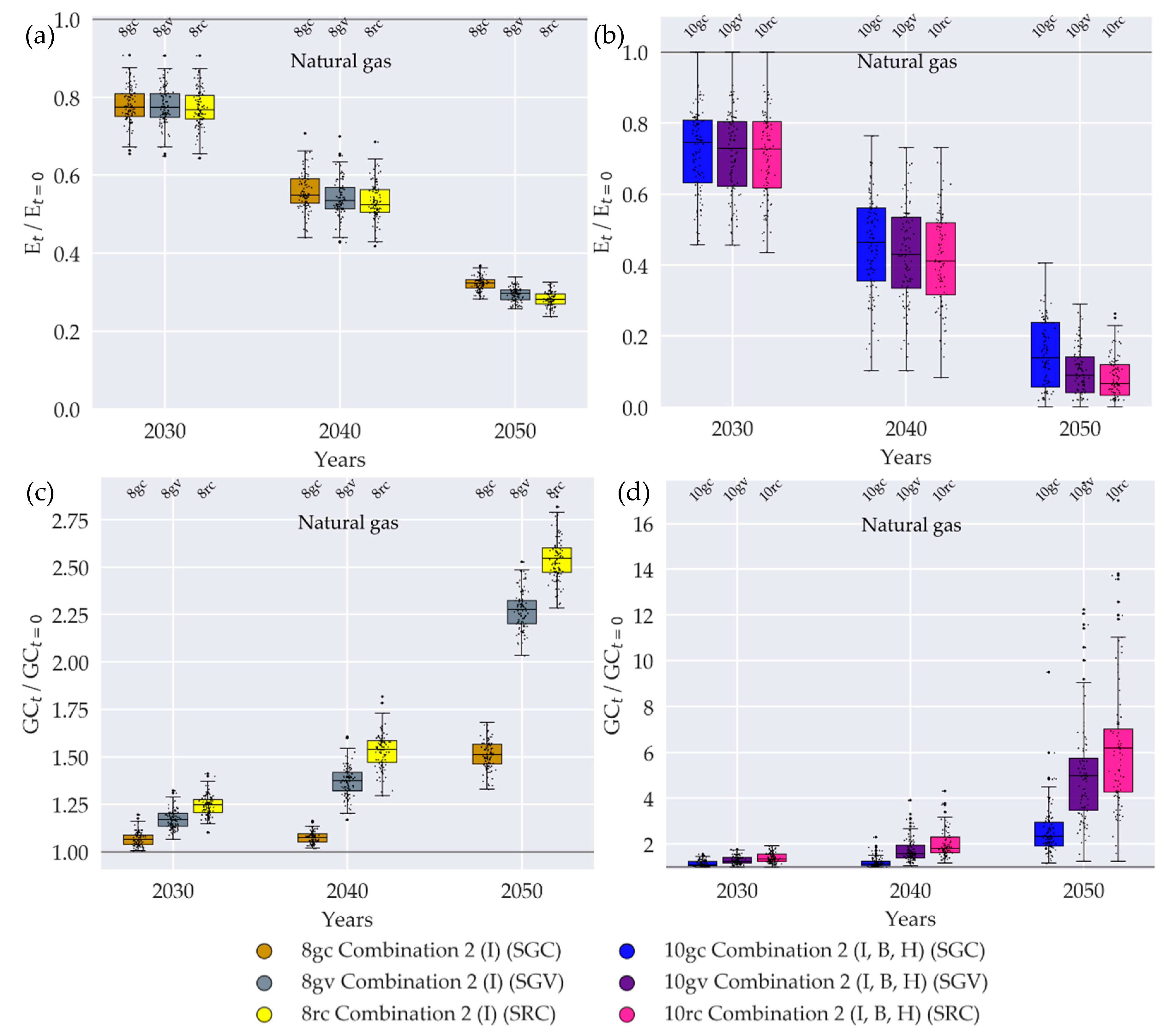
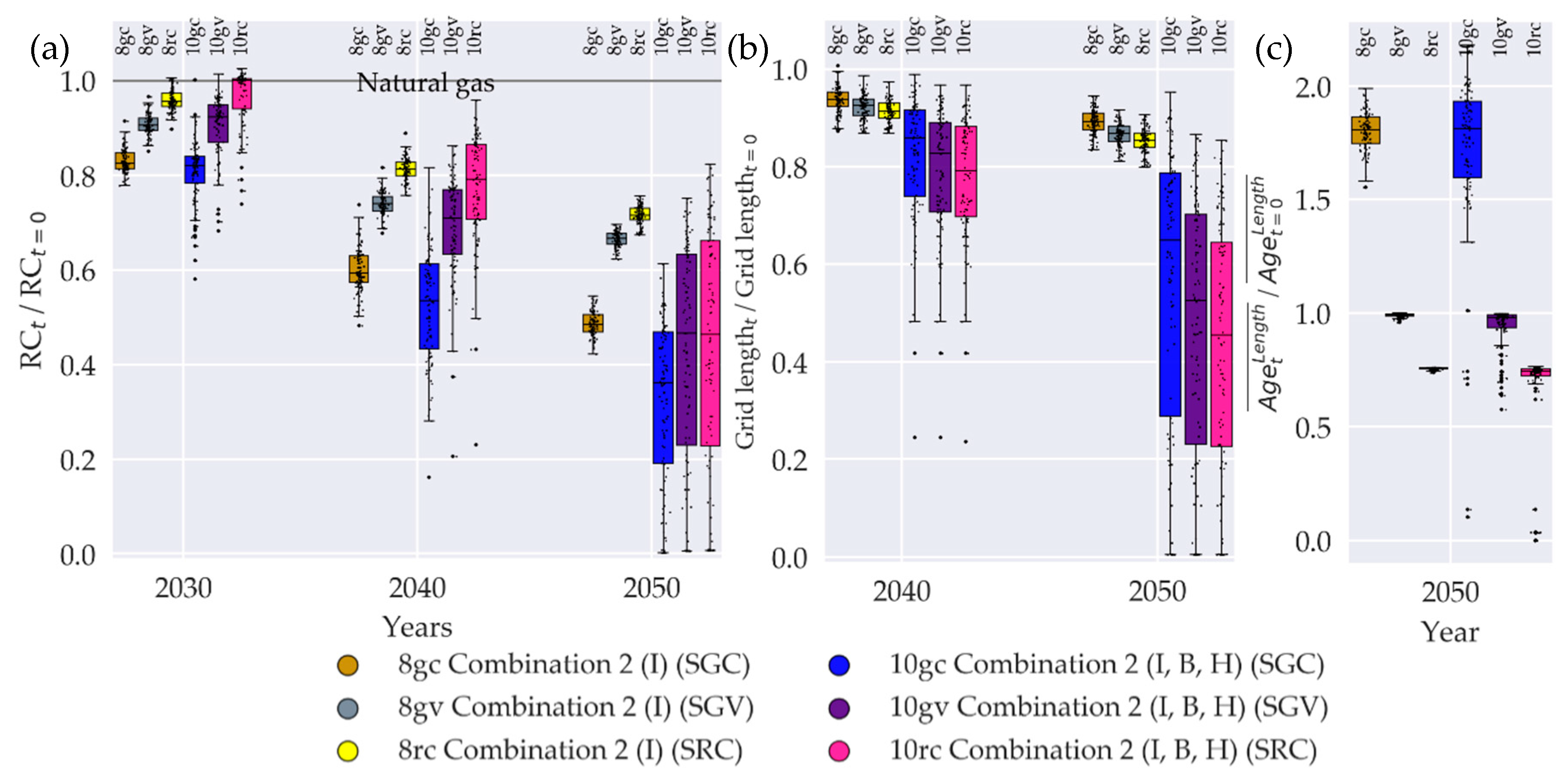
4.4. Case Study 4: The Influence of DNO Strategy Patterns on Grid Economy in Face of Decreasing Gas Demand

In the comparison of the three DNO strategies, we focus on the situation in gas grids, vary the gas DNO strategy, use the same strategy for the electricity DNO in all simulations and discuss the results for the natural gas sector. The effects on the electricity demand, the corresponding grid charges and the electricity DNO’s revenue cap are low; see the corresponding results in Appendix D.2 (electricity demand in Figure A5; grid charges in Figure A6; revenue cap in Figure A7).
Figure 12 shows the decrease in gas demand for the initial building and heating system configuration (I) in 12a and its variation (I, B, H) in 12b. The gas grid costs drop slower than the corresponding demand, leading to an increase in grid charges (Figure 12c,d). Thereby, the rate of change of grid charges depends on the DNO’s strategy and on the increase from the SGC via the SGV to the SRC strategy. The difference in grid charges finally leads to more investment in gas-based solutions for the SGC compared to the SRC strategy. We see this effect as the drop in gas demand is more pronounced for simulation 8rc compared with 8gc (a difference of the median of approximately 5% in 2050 in Figure 12a,b). For a variation of initial building and heating configuration (10gc, 10gv, 10rc) this can lead to a complete defection of the gas grid (Figure 12b); whereby the probability of occurrence for this scenario is higher in the long term when the DNO acts according to the SRC or SGV compared to the SGC strategy.
When comparing the gas grid charges of the initial building and heating configuration (I) in Figure 12c and its variation (I, B, H) in Figure 12d, it becomes clear that an interplay of an unfavorable DNO strategy (SRC) and a low initial house connection density to the gas grid can lead to a sharp increase in grid charges in 2050: We see a factor of 6.19 (median) in simulation 10rc, compared to 2.55 in simulation 8rc. In both cases, a change in strategy has a strong impact on network charges, which in turn can save the DNO’s business model in the long run: For the SGC strategy, the median is 2.32 in simulation 10gc and 1.51 in simulation 8gc (2050).
In the following, we discuss the consequences for the DNO’s business model based on Figure 13. Induced by the declining customer number, demand and grid length, we see a drop in revenues in all scenarios (Figure 13a), which is more pronounced for the SGC than for the SGV and SRC strategies. The decline goes along with a shift in CAPEX and OPEX caused by an interplay of the gas DNO’s and building owners’ decisions: The OPEX is a function of the energy supplied (Figure 12) and the grid length (Figure 13b). It therefore depends mostly on the building owner’s investment decision. The CAPEX is a function of the grid length and age. It therefore depends mainly on the DNO’s investment strategy and primarily determines the differences in revenue caps (Figure 13a). For CAPEX and OPEX see Figure A8 in Appendix D.2.
The change of grid length induced by line closure and new house connection measures is determined by the building owners’ investment decision. The remaining degree of freedom of the DNO decision is the determination of the renewal ratio, i.e., the choice of individual renewal measures. Lowering this ratio, as in the SGC strategy, leads to an increase of (length-weighted) grid age (Figure 13c). Increasing this ratio as in the SRC strategy induces the opposite effect: The DNO tries to keep its cost base at the starting level, and revenue shortfalls due to the loss of customers are compensated with an increase in the renewal ratio. As a result, the grid charges are relatively high in the SRC strategy and customers are increasingly replacing their gas-fired heating systems. In this way, more and more house connections and supply pipes are being shut down, which reduces the grid length (Figure 13b). Furthermore, the SRC strategy increases the risk of stranded investments, as the high revenue cap values are induced by CAPEX and thus the fixed assets. The relative OPEX of the SRC strategy in 2050 (0.33) is lower than in the SGC strategy (0.53).
As the decrease of grid length over time is slower than the decrease of the gas demand, the energy-related OPEX rises independently of the DNO strategy. This finally leads to a rise in grid charges in all strategies (Figure 12). In the SGC strategy, it is possible to a certain extent to compensate for the disproportionately rising costs in relation to the grid length by lowering the CAPEX, whereas the SRC strategy in particular allows these costs to rise. The results prove the feedback of the DNO strategy to the building owner’s decision:
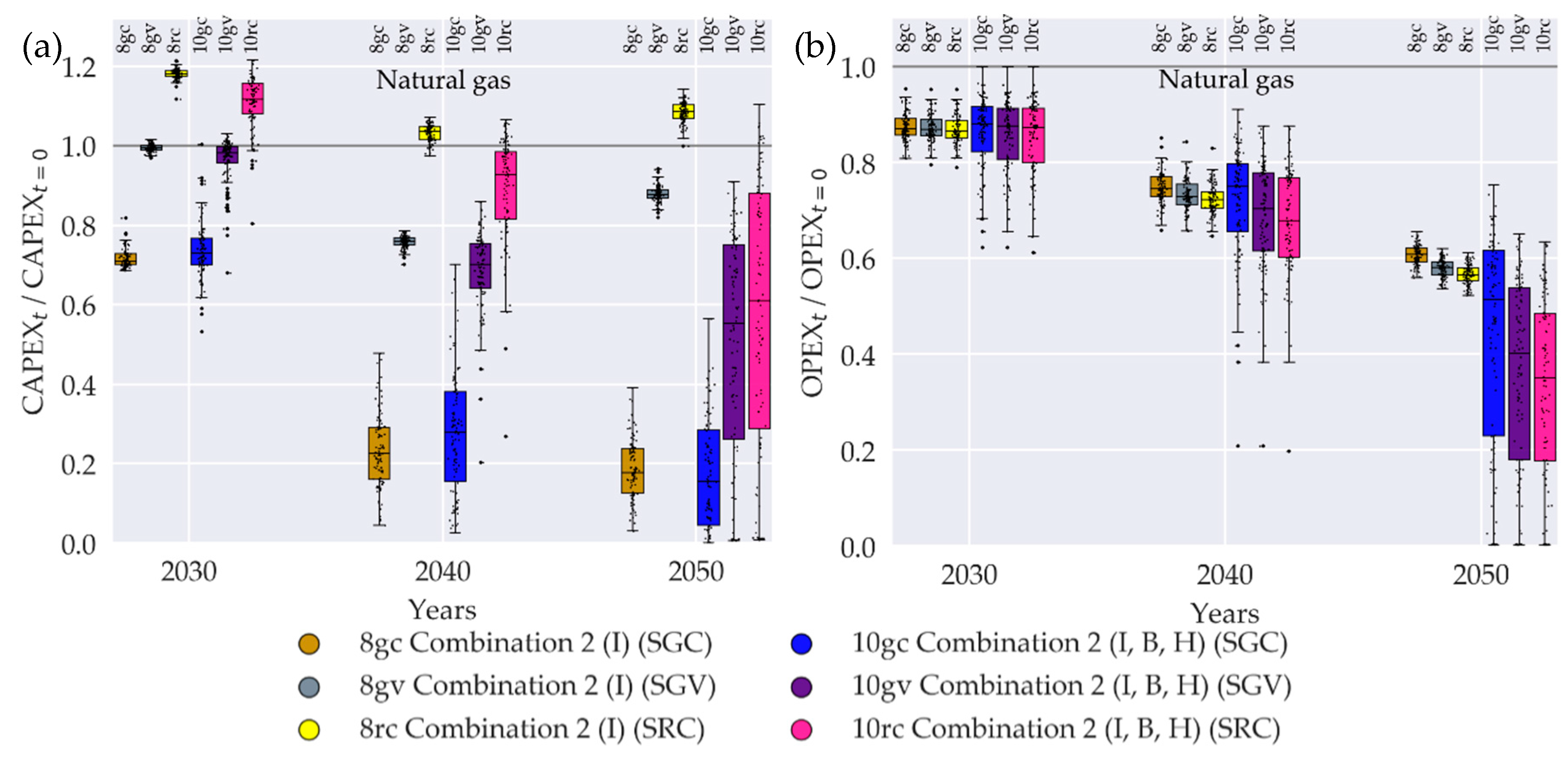
  • SRC: Due to the rise in grid charges, gas-bound systems are increasingly being substituted, resulting in a risk of a self-reinforcing effect, which in turn leads to an increased decline in the energy demand as well as network length. This could finally trigger the closure of the entire gas network.
  • SGC: The initial disadvantage concerning the lower cost base for the DNO resulting from a disproportionate decline in the CAPEX becomes less pronounced during the planning horizon, as the grid length and supplied energy and with that the OPEX are higher compared to the SRC strategy. In the long run, this strategy can help secure the business model and reduce the risk of a complete shutdown, as a comparison of network lengths shows.

5. Conclusions

Our simulation provides two main innovations in modeling: We integrate a cash flow calculation and a grid planning model into one DNO model. This enables us to assess the implications of different DNO strategic patterns on grid measures and grid charges.
The results of the case studies with the joint MAS simulation give some new insights into the interrelated system between building owners’ and the DNO’s investment decisions: Some configurations of endogenous economic, regulatory, and technical triggers induces the substitution of gas-bound heating systems mostly with electric heat pumps. Due to the sensitivity of building owners’ investment decisions to gas price fluctuations and the sensitivity of gas grid charges on gas demand, a self-reinforcing feedback loop starts and accelerates the defection of the gas grid (Figure 14). A change in the gas DNO’s strategy can reduce but not stop this feedback. These implications are relevant for DNOs, policy makers, and building owners.

5.1. Implications for Building Owners

Due to the existing gas network and the building and heating system configuration, gas-fired heating systems are predominantly used in the investigated area, while insulation measures and electric heat pumps appear unattractive. The development is changing when the solution space is limited or steered by triggers: Most single triggers, like CO2 pricing, an increased heat pump efficiency, government subsidies, or a reduction of electricity grid charges have a minor influence on the decision. The application of an energy-efficiency constraint shows large effects. Dependent on the design of the energy-efficiency constraint, electrical heat pumps, solar thermal plants, and surface insulation measures comes into play. Ambitious CO2-efficiency targets are associated with high costs; see Figure A4 in Appendix D.1.
The results indicate gas grid charges as a trigger element for retrofit decisions: For some building and heating configurations, the development of gas grid charges triggers an increase instead of a decrease in gas demand. In the worst case, this could lead to complete grid defection. Under the current political CO2 emission targets and the CO2 footprint of the natural gas supply, a financial risk for building owners arises when choosing a gas-based heating system: Future CO2 prices and grid charges are difficult to predict and the energy-related costs can rise sharply during the life-cycle. Furthermore, it is possible that fossil-fired plants will be banned during their lifetime [105]. Our model does not cover these economic risks, due to from incomplete information. The building owner can reduce the risk by making him or herself less dependent on energy supply through improved building insulation measures, self-generating systems or efficient heating systems, such as heat pumps. These desolidarization efforts can already be observed in practice and are part of studies [29] that are so far mostly focused on the situation in the electricity grid.

5.2. Implications for Natural Gas and Electricity Distribution Grid Opteraters

The results show that the disordered structure inherent to grid-based infrastructure leads to an increase in length-related grid costs, i.e., grid charges in scenarios with a strong decrease in gas demand. A change of the DNO’s strategy can only counteract this effect to a limited extent. The short-term more profitable gas DNO strategy (SRC) increases the risk of a closure of the entire gas network in the long-term due to the feedback effect via grid charges. A strategy (SGC) that is less profitable for the DNO, but more in the public interest, contributes to the long-term maintenance of the gas grid infrastructure. A decision on the future of the gas grid infrastructure taken at macroeconomic level could reduce these economic risks.
We see the postulated feedback loop not only between the gas DNO and the buildings. There is also an interdependency between the gas and electricity DNO’s revenue caps, due to the competition between gas burners and electrical heat pumps. In this context, the gas-based heating systems act as a trigger element for the tilting effects on the DNO’s cost base. For that reason, the DNO could incentivize building owners to install gas-based systems in the future. In addition to the adaptation of the investment and operation strategy, this could help maintain the gas grids for some areas.

5.3. Implications for Policy Makers

We have shown that the use of single triggers, such as regulatory constraints, levy systems or state subsidy programs, mostly favors individual types of measures or systems but contributes little to the overall goal of CO2 reduction. This effect can be mitigated by designing state measures for technology neutrally, without a pronounced steering effect for specific building envelope measures or heating systems. The formulation of reduction targets for primary energy demand or CO2 as well as the introduction of levy and subsidy systems, such as CO2-pricing, represent technology-neutral alternatives.
In scenarios with a decreasing gas demand, the DNO strategy can contribute to maintaining the gas grid infrastructure. According to the actual incentive regulation system in Germany, DNOs apply the SRC or the SGV strategy with which they increase their business risk through grid defection in the long-term in such scenarios. This poses a risk to society, since gas networks are seen as a flexibility option for volatile electricity production [23]. From a macrosocial point of view, the question arises whether gas networks are necessary in the future energy system. If not, a stepwise shutdown with regulatory support could guarantee a stable supply within the transformation; if so, appropriate business incentives for gas DNOs could reduce the risk of grid defection [21,22].

5.4. Further Research

Until now, the role of a change in gas grid costs due to decreasing demand or titling effects has not been sufficiently considered in energy system analyses [16,17,18,19]. The increase of grid charges is mainly induced by the non-linear dependency between grid length and customer number or demand. Models are available to consider this aspect in energy system analysis [22].
If more and more customers leave the gas grid in the future, the risk of stranded investments on the DNO side will increase. Knowledge about the future development of the building stock could help qualify this risk. The investment theory offers numerous methods for the valuation of investments under uncertainty and the quantification of this risk [108]. They could be adapted to gas grids to consider age, importance, and risk when choosing renewal measures.
The results also imply an interdependence between gas DNO and electricity DNO. For society, the question arises whether a joint cost-base for the electricity and gas grids, can help to reduce the long-term risk of gas grid defection. This instrument would provide the basis for a cross-sectoral infrastructure charge, which could help maintain the gas grid as a flexibility option.

Supplementary Materials

The following are available online at https://0-www-mdpi-com.brum.beds.ac.uk/2071-1050/12/13/5315/s1, Section A.1: Thermal Building Model—Calculation of the Building Heat Load, Section A.2: Thermal Building Model—Domestic Hot Water Generation and Additional Heat Losses and Wins, Section A.3: Solar Thermal Model, Section A.4: Building Surface Model—Calculation of Specific Building Surface Investment Expenditures and Heat Transmission Coefficients, Section A.5: Preprocessing Procedure for the Calculation of the Building Individual Investment Expenditures for the Heating System, Section B.1: Architecture of the Gas and Electricity Network Operator Model, Section B.2: Grid Measures of the Gas and Electricity DNO, Section C.1: Building, heating system and solar thermal parameters, Section C.2: Parameters of the Single Seeds: Date of Investment, Building Age Classes, Heating System Types & Surface Insulation Constraint, Figure S1: Scheme of data prorogation in regard to the energy demand and economic parameters implemented for natural gas and electricity grid, Table S1: Parameters of the available solar thermal plants, Table S2: Specific investment expenditures per building part based on [75], Table S3: Considered cost drivers for the heating system, Table S4: Available building heating systems, Table S5: Heat transmission coefficients of the energy efficiency constraint for each building part [100], Table S6: Building properties of the used building types and corresponding energy efficiency constraint, Table S7: Initial building heating system types base on [95,107,109], Table S8: Surface areas of building types [61,62], Table S9: U-Values of building types [61,62], Table S10: Heating circuit temperatures for the corresponding building age classes and heating systems, Table S11: Date of investment of all buildings in the data set, Table S12: Building age class of all buildings in the data set, Table S13: Heating system type of all buildings in the data set, Table S14: Surface insulation constraint (66% of buildings).

Author Contributions

Conceptualization, D.T. and T.M.K.; data curation, P.H.; Formal analysis, M.B.; funding acquisition, T.M.K. and M.B.; investigation, D.T. and P.H.; methodology, D.T.; software, P.H.; supervision, M.B.; visualization, D.T.; writing—original draft, D.T.; writing—review and editing, T.M.K. and M.B. All authors have read and agreed to the published version of the manuscript.

Funding

This research received no external funding.

Acknowledgments

We would like to thank the Stadtwerke Bamberg energy and water supply company, Bamberg, Germany, for providing us the data of loads, grids, and costs components that form the basis for this work.

Conflicts of Interest

D.T. is an employee of the Stadtwerke Bamberg GmbH. The authors declare no conflict of interest.

Appendix A Nomenclature

Table A1. List of acronyms.
AcronymNameAcronymName
AWHPAir water heat pumpMASMulti-agent simulation
BESBuilding energy systemMFHMore family house
BEBuilding envelopeMILPMixed integer linear program
BBuilding age classMPMedium pressure
BOBuilding ownerMVMedium voltage
CAPEXCAPEXOCBOil condensing boiler
CO2Carbon dioxideOPEXOPEX
COPCoefficient of performance (heat pumps)OSMOpen street maps
DHWDomestic hot waterPBPellet burner
DNODistribution network operatorPFPresent value factor
EEnergyRFAReference floor area
EDHElectrical direct heatingRBVRest book value
EUEuropean UnionRCRevenues cap
GCGrid chargesSTESolar thermal plant
GCBGas condensing boilerSFHSingle family house
GWHPGround water heat pumpSGCStable grid charges
HType of heating systemsSGVStable grid value
IDate of investmentSRCStable revenue cap
IQDInter quantile distanceSTESolar thermal energy plant
IWUInstitute Housing and EnvironmentTHTerraced house
LPLow pressureWODeprecations (or write-offs)
LVLow voltage

Appendix B Building Retrofit Model

Appendix B.1. Nomenclature

Table A2. Nomenclature of formula symbols.
ParameterDescription [unit]ValueSource
Components of the expenditures
c 𝒿 B Total expenditures for heating within the technical lifetime of the heating system [€]
c 𝒿 BE Investment expenditures for the building insulation retrofit [€]
c 𝒿 BES Investment expenditures for the change of the heating system and technical building equipment [€]
c 𝒿 EN Expenditures for energy procurement over the technical lifetime of the heating system [€]
c 𝒿 M Expenditures for maintenance over the technical lifetime of the heating system [€]
Parameters
A 𝒿 E Building surface area [m²]Corresponding values are shown in Table S6 in the supplementary materials, based on [61,62,100]
T 𝒿 N Yearly usage hours of the heating system [h]
S 𝓭 , 𝒿 BE Design-relevant building heat load (for heating system) (thermal ventilation and transmission losses) [kW]Thermal models are shown in parts A1, A2, A3 in the supplementary materials, based on [62,73,74,76,82,83,95]
S 𝒿 S Heat load for: Radiation losses, internal wins, heat distribution losses, auxiliary energy [kW]
S 𝓼 , 𝒿 STE Heat load thermal solar plant [kW]
S 𝒿 DHW Heat load for domestic hot water generation [kW]
M 𝓴 BES Specific yearly expenditures for maintenance of the heating in percent of investment expenditure [-]
M 𝓼 STE Specific yearly expenditures for maintenance for the solar thermal plant in percent of investment expenditure [-]
E 𝓴 BES Plant expenditure figure of the heating systems
B c , 𝓴 EC Energy carrier of the heating system (Binary decision parameter)
C 𝒿 BEvar Specific variable investment expenditures for a building surface retrofit [€/(m²·cm)]Calculation is shown in A4 in the supplement materials; the corresponding values are shown in Tables S5, S6, S8, S9 in the supplementary materials, based on [61,62,75,100]
C 𝒿 BEfix Specific fix investment expenditures for a building surface retrofit [€/m²]
D 𝓭 D Insulation thickness [cm]0–30
C 𝓴 BESvar Specific variable expenditures for the heating system [€/kW]Calculation is shown in A5 in the supplement materials; the corresponding values are shown in Tables S3, S4, S7, S9 in the supplementary materials, based on [37,61,62,75,76,77,78,95,106,107,109]
C 𝓴 ,   𝒿 BESfix Specific fix expenditures for the heating system [€]
C 𝓼   STEvar Specific variable expenditures for the solar thermal plant [€/kW]
C 𝓼 STEfix Specific fix expenditures for the solar thermal plant [€]
C c , 𝓉 EC Specific yearly energy related expenditures (tax + procurement + grid charges) [€/kWh]
C c , 𝓉 Proc Specific energy procurement costs Electricity [€/kWh]7.61[79]
Natural gas [€/kWh]3.13[79]
Oil [€/L]0.506[80,110,111]
Pellet [€/kg]0.0173[81,112]
C c , 𝓉 Tax Energy related taxes and duties Electricity [€/kWh]16.02[79]
Natural gas [€/kWh]1.64[79]
Oil [€/L]0.169[80,110,111]
Pellet [€/kg]0.0173[81,112]
EM c , 𝓉 EC Specific CO2-emissions per energy carrier [kg/kWh]Electricity (linear decrease to 0.103 in 2050)0.462[113,114]
Natural gas0.202[115]
Oil0.294
Pellet0.023
HV c Heating value Natural gas [kWh/m³]11.42[116]
Oil [kWh/liter]11.27[116]
Pellet [kWh/kg]5.27[117]
F c P Primary energy factorElectricity1.8[76]
Natural gas1.1
Oil1.1
Pellets0.2
Q 𝒿 H init Initial yearly end energy demand of a building
EM 𝒿 init Initial yearly CO2 emissions of a building
Q 𝒿 P EnEV Upper bound for the yearly primary energy demand considering the energy efficiency constraint
S 𝒿 T EnEV Upper bound for the heat load considering the energy efficiency constraint
PF Present-value factor31
Variables
b 𝓭 , 𝒿 B E Building surface retrofit 𝒹 in house 𝒿 (Binary decision variable)
b k ,   𝒿 B E S Heating system 𝓀 in house 𝒿 (Binary decision variable)
b 𝓼 , 𝒿 S T E Solar thermal plant 𝓈 in house 𝒿 (Binary decision variable)
e c , 𝓉 Heating Energy for heating applications in year 𝓉 in gas or electricity grid [kWh/a]
c c , 𝓉 G C Grid charges gas or electricity in year 𝓉 [€/kWh]
Indices and sets
𝓭 D An insulation thickness standard 𝒹 of all standards 𝒟
𝓭 𝒫 Surface part 𝓅 of all building surface parts 𝒫
𝓺 Q 𝓅 A sub-part 𝓺 of all sub-parts Q of a building envelope part 𝓅
𝓴 𝒦 A heating system type 𝓀 of all heating system types 𝒦
c   ϵ   𝒞 An energy carrier 𝒸 of all carriers 𝒞
𝓼 𝒮 A solar thermal plant 𝓈 of all available types and sizes 𝒮
𝒿   ϵ   𝒥 A building 𝒿 of all buildings 𝒥 connected to the grid
Parameters of the supplements (derivations and tables)
C 𝓴 B H S Investment expenditures for heating surfaces and pipe system (per RFA) [€/m²]
H 𝒿 Transmission heat loss [W/K]
H 𝒿 T Transmission heat loss [W/K] (Transmission)
H 𝒿 V Transmission heat loss [W/K] (Ventilation)
U 𝒿 T Heat transmission coefficient [W/(m²·K)]
Δ U 𝒿 TB Heat transmission coefficient for thermal bridges [W/(m²·K)]
U 𝒿 0 Initial heat transmission coefficient [W/(m²·K)]
U 𝒿 , 𝓅 ESP Heat transmission coefficient of a building surface part [W/(m²·K)]
ϑ Out Outdoor temperature [°C]
ϑ In Indoor temperature [°C]
Δ T nom Design relevant temperature difference outdoor versus indoor [°C]
A 𝒿 E Building surface area [m²]
A 𝒿 , 𝓅 EP Area of a building surface component [m²]
A 𝓺 ESP Area of a sub-part of a building surface component [m²]
F 𝓼 STEred Reduction factor of the solar thermal plant [–] (reduction of the energy demand for DHW generation)
A STE Area of the solar thermal plant [m²]
STE yield Yearly average solar yield [kWh/(m²·a)]
V 𝒿 𝓴 , 𝓼 DHW Capacity of the domestic hot water tank [liter]

Appendix B.2. Constraints of the Building Retrofit Model

We constrained the number of measures per category in each simulation, considering A1, A2, and A3. The optimizer can choose a building surface insulation measure:
𝒿 J : d D b 𝓭 , 𝒿 BE 1
The optimizer has to replace the heating system:
𝒿 J : 𝓴 K b 𝓴 , 𝒿 BES = 1
The optimizer can choose a solar thermal plant:
𝒿 J : 𝓼 S b s , 𝒿 STE 1
In each simulation we set the initial yearly CO2 emissions (A4) and the end energy demand (A5) as upper bounds:
𝒿 J : 𝓴 K ( ( ( 𝓭 D ( S 𝓭 , 𝒿 BE b 𝓭 , 𝒿 BE ) + S 𝒿 S ) b 𝓴 , 𝒿 BES + 𝓼 S ( S 𝒿 DHW ( S 𝓼 , 𝒿 STE b 𝓼 , 𝒿 STE ) ) b 𝓴 , 𝒿 BES   ) T 𝒿 N E 𝒿 BES 𝓴 C ( B c , 𝓴 EC F 𝓴 P EM c EC ) ) EM 𝒿 init
𝒿 J : 𝓴 K ( ( ( 𝓭 D ( S 𝓭 , 𝒿 BE b 𝓭 , 𝒿 BE ) + S 𝒿 S ) b 𝓴 , 𝒿 BES + 𝓼 S ( S 𝒿 DHW ( S 𝓼 , 𝒿 STE b 𝓼 , 𝒿 STE ) ) b 𝓴 , 𝒿 BES   ) T 𝒿 N E 𝓴 BES ) Q 𝓴 H init
In our case-studies in simulations 3, 8–10 we constrained the yearly primary energy demand to the corresponding demand Q 𝒿 P EnEV , calculated based on the energy-efficiency targets of [100] (for the Q 𝒿 P EnEV values see Supplement C, Table S6). The optimizer can freely choose the type of measure.
𝒿 J : 𝓴 K ( ( ( 𝓭 D ( S 𝓭 , 𝒿 BE b 𝓭 , 𝒿 BE ) + S 𝒿 S ) b 𝓴 , 𝒿 BES + 𝓼 S ( S 𝒿 DHW ( S 𝓼 , 𝒿 STE b 𝓼 , 𝒿 STE ) ) b 𝓴 , 𝒿 BES   ) T 𝒿 N E 𝓴 BES F c P ) Q 𝒿 P EnEV
We also added a restriction to oblige building owners to insulate their building envelope in order to reach the energy-efficiency goals according to [100]. (In simulation 3 this was applied for 100% of the buildings, while in simulations 8–10 it was applied for 66% of the building)
𝒿 J : 𝓴 K ( 𝓭 D ( S 𝓭 , 𝒿 BE b 𝓭 , 𝒿 BE ) ) S 𝒿 T EnEV

Appendix C Gas and Electricity Network Operator Model

Appendix C.1. Nomenclature

Table A3. Nomenclature of formula symbols.
ParameterDescription [unit]ValueSource
GasElectricity
Cost components of the revenue cap
α c , 𝓉 C A P E X Capital expenditures gas or electricity [€]
α c , 𝓉 O P E X Operational expenditures gas or electricity [€]
α c , 𝓉 E C Calculated return on equity gas or electricity [€]
α c , 𝓉 B C Interest on borrowed capital gas or electricity [€]
α c T a x Calculated trade tax gas or electricity [€]
α c , 𝓉 D e p r Calculated interest on borrowed capital gas or electricity [€]
α c , 𝓉 O C Operational costs gas or electricity [€]
α c , 𝓉 L C Loss costs gas or electricity [€]
α c , 𝓉 U p G C Upstream grid charges gas or electricity [€]
α c , 𝓉 C o n c Concession fees gas or electricity [€]
Parameters
R   EC Interest rate equity capital of line ℓ0.0691 *0.0691 *
Q   EC Amount of equity capital of line ℓ0.400.40[21]
R   BC Interest rate borrowed capital of line ℓ0.035 *0.035 *
Q   BC Amount of borrowed capital of line ℓ0.600.60[21]
R Tax Trade tax rate0.14 *0.14 *
T TL Technical lifetime of a line [a]4045[99,118]
T Planning Planning horizon [a]3131
C 𝓉 UpGCG Specific costs of upstream grid charges [€/kWh]0.0030 *0.025 *
C 𝓉 Conc Specific costs for concession fees [€/kWh]0.0023 *0.011 *
C LC Specific lost costs [€/kWh]0.0080 *0.044 *
F Loss Loss factor0.00 *0.026 *
C LRC Specific operational costs [€/m]5.0 *7.9 *
E c , 𝓉 AnyOther Any other energy in year 𝓉 in gas or electricity grid [kWh/a] (calculated based on the RFA)0 * [kWh/ (m²·a)]25 * [kWh/(m²·a)]
Variables
T   Init Line age at the begin of planning horizon [a] *
C   I Historical acquisition expenditures for line ℓ [€/m] *
L Line length of line ℓ [m] *
A M e a n I n i t Length-weighted average age of the grid [a]
RBVF , c Rest book value factor of line ℓ in year 𝓉 as a function of the binary decision variables
c c ,     c GC Grid charges gas or electricity in year 𝓉 [€/kWh]
e c , 𝓉 Heating Energy for heating applications in year 𝓉 in gas or electricity grid [kWh/a]
Indices and sets
𝒿   ϵ   J A building 𝒿 of all buildings 𝒥 connected to the grid
  ϵ   A line ℓ of all lines in the grid
c   ϵ   T A year 𝓉 within the planning horizon 𝒯
c   ϵ   C An energy carrier 𝒸 of all carriers 𝒞
Investment expenditure for new construction of grid assets
C T Investment expenditures transformer substation MV/LV [€]0.25 MVA 67,000 *
0.4 MVA 74,000 *
0.63 MVA 83,000 *
C EL Investment expenditures electrical lines [€/m]NAYY 4x50 SE 114 *
NAYY 4x120 SE 114 *
NAYY 4x150 SE 114 *
C P Investment expenditures pressure regulator station [€]20,000 *
C GP Investment expenditures gas pipes [€/m]40 ST63 *
80 ST163 *
100 ST209 *
150 ST287 *
200 ST360 *
25 PE 100 SDR 1140 *
50 PE 100 SDR 1179 *
90 PE 100 SDR 17200 *
* Values are chosen on the basis of local conditions in Bamberg or the DNO (Germany 2019).

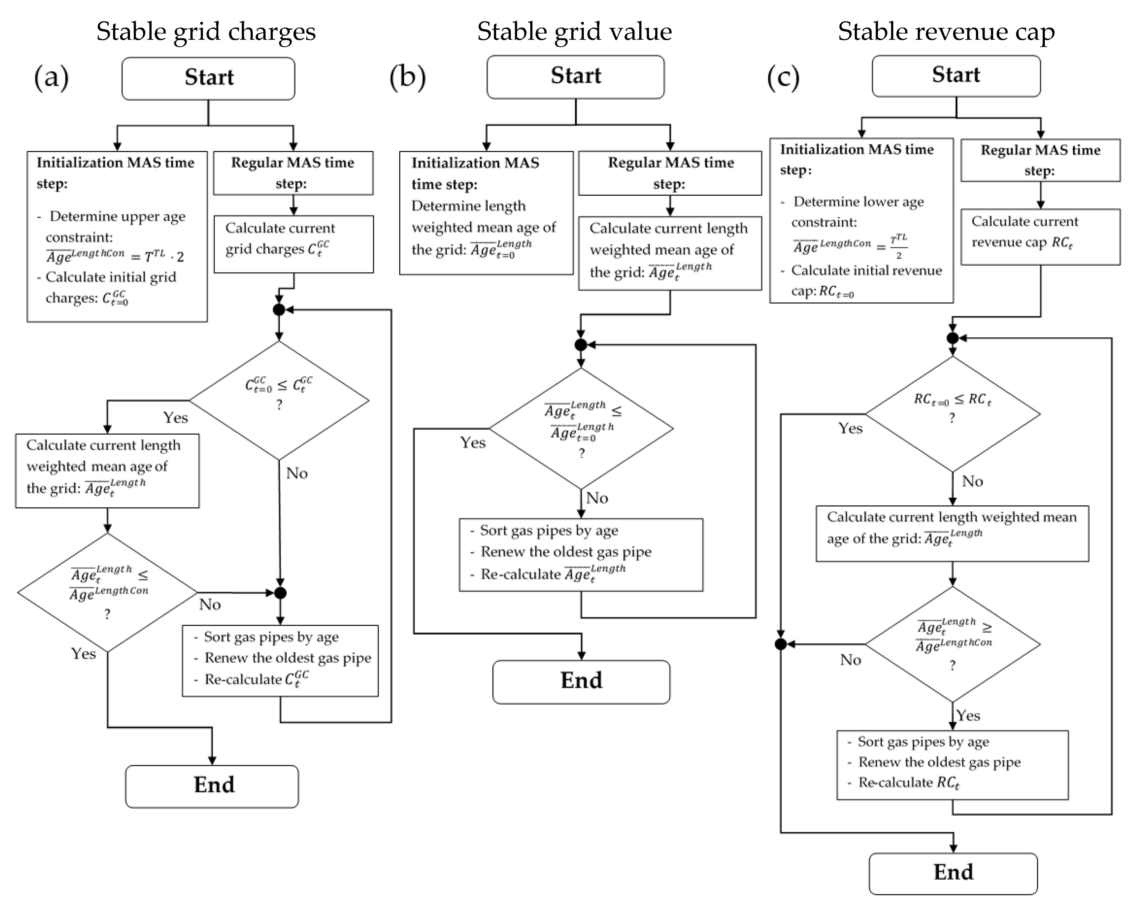
Appendix C.2. Flowcharts of the Investment Strategies

Figure A1. Flowchart for a time step of gas DNO strategies: (a) stable grid charges; (b) stable grid value; and (c) stable revenue cap (the stable grid value strategy (b) is analogously applied in the electricity DNO).
Sustainability 12 05315 g0a1

Appendix D Case studies

Appendix D.1. Additional Results: Possible Triggers for a Deacrease in Gas Demand

Figure A2. Relative electricity demand in projected years for (a) different triggers and their combinations; (b) a variation of building age classes and heating systems. (Dots: individual seeds; boxes: median and 25%/75% percentiles of the resulting distribution; whiskers: +/− 1.5 IQD).
Sustainability 12 05315 g0a2
Figure A3. Relative electricity grid charges in projected years for (a) different triggers and their combinations (b) a variation of building age and heating systems. (Dots: individual seeds; boxes: median and 25%/75% percentiles of the resulting distribution; whiskers: +/− 1.5 IQD).
Sustainability 12 05315 g0a3
Figure A4. (a) Mean value of CO2 emissions of all retrofitted buildings in the year of renovation; (b) mean value of total costs of retrofitting and operation for all buildings (capital + operational expenditures). (Dots: individual seeds; boxes: median and 25%/75% percentiles of the resulting distribution; whiskers: +/− 1.5 IQD).
Sustainability 12 05315 g0a4

Appendix D.2. Additional Results: The Influence of DNO Strategy Patterns on Grid Economy in Face of Decreasing Gas Demand

Figure A5. Relative electricity demand in projected years with a comparison of different gas DNO strategies with (a) a variation of the date of investment (I); (b) a variation of date of investment, building age type, and heating system type (I, B, H). (Electricity DNO strategy in all simulations: “stable grid value”). (Dots: individual seeds; boxes: median and 25%/75% percentiles of the resulting distribution; whiskers: +/− 1.5 IQD).
Sustainability 12 05315 g0a5
Figure A6. Relative electricity grid charges in projected years with a comparison of different gas DNO strategies with (a) a variation of the date of investment (I); (b) a variation of date of investment, building age type, and heating system type (I, B, H). (Electricity DNO strategy in all simulations: “stable grid value”). (Dots: individual seeds; boxes: median and 25%/75% percentiles of the resulting distribution; whiskers: +/− 1.5 IQD).
Sustainability 12 05315 g0a6
Figure A7. Relative value of the electricity DNO’s revenue cap in projected years with a comparison of different gas DNO strategies (electricity DNO strategy in all simulations: “stable grid value”). (Dots: individual seeds; boxes: median and 25%/75% percentiles of the resulting distribution; whiskers: +/− 1.5 IQD).
Sustainability 12 05315 g0a7
Figure A8. Relative values in projected years with a comparison of different gas DNO strategies for (a) CAPEX and (b) OPEX of the gas DNO. (Dots: individual seeds; boxes: median and 25%/75% percentiles of the resulting distribution; whiskers: +/− 1.5 IQD).
Sustainability 12 05315 g0a8

References

  1. REN21 Renewable Energy Policy Network for the 21st Century. Renewables 2018—Global Status Report; REN21 Renewable Energy Policy Network for the 21st Century: Paris, France, 2018. [Google Scholar]
  2. Honoré, A. Decarbonisation of Heat in Europe: Implications for Natural Gas Demand; Oxford Institute for Energy Studies: Oxford, UK, 2018. [Google Scholar]
  3. Mateo, C.; Frías, P.; Tapia-Ahumada, K. A comprehensive techno-economic assessment of the impact of natural gas-fueled distributed generation in European electricity distribution networks. Energy 2020, 192, 116523. [Google Scholar] [CrossRef]
  4. Kassai, M. Prediction of the HVAC energy demand and consumption of a single family house with different calculation methods. Energy Procedia 2017, 112, 585–594. [Google Scholar] [CrossRef]
  5. Kassai, M. Experimental investigation on the effectiveness of sorption energy recovery wheel in ventilation system. Exp. Heat Transf. 2018, 31, 106–120. [Google Scholar] [CrossRef]
  6. Vazinram, F.; Hedayati, M.; Effatnejad, R.; Hajihosseini, P. Self-healing model for gas-electricity distribution network with consideration of various types of generation units and demand response capability. Energy Convers. Manag. 2020, 206, 112487. [Google Scholar] [CrossRef]
  7. Jianhong, Y. Analysis of sustainable development of natural gas market in China. Nat. Gas Ind. B 2018, 5, 644–651. [Google Scholar] [CrossRef]
  8. Ailin, J. Progress and prospects of natural gas development technologies in China. Nat. Gas Ind. B 2018, 5, 547–557. [Google Scholar] [CrossRef]
  9. Mastorakos, S.; Madrigal, J.; Duffy, E.; Ebertin, M.; Bosso, E. The Future of Natural Gas in the United States; United States Ecologic Institute: Washington, DC, USA, 2017. [Google Scholar]
  10. Feijoo, F.; Iyer, G.C.; Avraam, C.; Siddiqui, S.A.; Clarke, L.E.; Sankaranarayanan, S.; Binsted, M.T.; Patel, P.L.; Prates, N.C.; Torres-Alfaro, E.; et al. The future of natural gas infrastructure development in the United states. Appl. Energy 2018, 228, 149–166. [Google Scholar] [CrossRef]
  11. Costello, K.W. Why natural gas has an uncertain future. Electr. J. 2017, 30, 18–22. [Google Scholar] [CrossRef]
  12. Mac Kinnon, M.A.; Brouwer, J.; Samuelsen, S. The role of natural gas and its infrastructure in mitigating greenhouse gas emissions, improving regional air quality, and renewable resource integration. Prog. Energy Combust. Sci. 2018, 64, 62–92. [Google Scholar] [CrossRef]
  13. Speirs, J.; Balcombe, P.; Johnson, E.; Martin, J.; Brandon, N.; Hawkes, A. a greener gas grid: What are the options. Energy Policy 2018, 118, 291–297. [Google Scholar] [CrossRef]
  14. Qadrdan, M.; Fazeli, R.; Jenkins, N.; Strbac, G.; Sansorn, R. Gas and electricity supply implications of decarbonising heat sector in GB. Energy 2019, 169, 50–60. [Google Scholar] [CrossRef]
  15. McGlade, C.; Pye, S.; Ekins, P.; Bradshadw, M.; Watson, J. The future role of natural gas in the UK: A bridge to nowhere? Energy Policy 2018, 113, 454–465. [Google Scholar] [CrossRef] [Green Version]
  16. Henning, H.M.; Palzer, A. Energiesystem Deutschland 2050; Fraunhofer-Institut für Solare Energiesysteme (ISE): Freiburg, Germany, 2013. [Google Scholar]
  17. Deutsch, M.; Gerhardt, N.; Sandau, F.; Becker, S.; Scholz, A.; Schumacher, P.; Schmidt, D. Wärmewende 2030—Schlüsseltechnologien zur Erreichung Der Mittel- und Langfristigen Klimaschutzziele im Gebäudesektor—Eine Studie im Auftrag Der Agora Energiewende; Fraunhofer-Institut für Windenergie und Energiesystemtechnik (IWES): Bremerhaven, Germany; Fraunhofer-Institut für Bauphysik (IBP): Stuttgart, Germany, 2017. [Google Scholar]
  18. Ziesing, H.J.; Repenning, J.; Emele, L.; Blanck, R.; Böttcher, H.; Dehoust, G.; Förster, H.; Greiner, B.; Harthan, R.; Henneberg, K.; et al. Klimaschutzszenario 2050—2. Endbericht—Eine Studie im Auftrag des Bundesministeriums für Umwelt, Naturschutz, Bau und Reaktorsicherheit; Institut für Angewandte Ökologie e.V. (Öko-Institut): Berlin, Germany; Fraunhofer-Institut für System- und Innovationsforschung (ISI): Karlsruhe, Germany, 2015. [Google Scholar]
  19. Gerhardt, N.; Sandau, F.; Scholz, A.; Hahn, H.; Schumacher, P.; Sager, C.; Bergk, F.; Kämper, C.; Knörr, W.; Kräck, J.; et al. Interaktion EE-Strom, Wärme und Verkehr—Analyse Der Interaktion Zwischen den Sektoren Strom, Wärme/Kälte und Verkehr in Deutschland in Hinblick auf Steigende Anteile Fluktuierender Erneuerbarer Energien im Strombereich unter Berücksichtigung der Europäischen Entwicklung—Ableitung von Optimalen Strukturellen Entwiklungspfaden für den Verkehrs- und Wärmesektor; Fraunhofer-Institut für Windenergie und Energiesystemtechnik (IWES): Bremerhaven, Germany; Fraunhofer-Institut für Bauphysik (IBP): Stuttgart, Germany; Institut für Energie- und Umweltforschung (ifeu): Heidelberg, Germany; Stiftung Umweltenergierecht: Würzburg, Germany, 2015. [Google Scholar]
  20. Seack, A.; Kays, J.; Rehtanz, C. Integral distribution grid planning process considering the impact of heat pump systems. In Proceedings of the 2016 Power Systems Computation Conference (PSCC), Genoa, Italy, 20–24 June 2016. [Google Scholar] [CrossRef]
  21. Däuper, O.; Strasser, T.; Lange, H.; Tischmacher, D.; Fimpel, A.; Kaspers, J.; Koulaxidis, S.; Warg, F.; Baudisch, K.; Bergmann, P.; et al. Wärmewendestudie—Die Wärmewende und Ihre Auswirkungen auf Die Gasverteilnetze; Becker Büttner Held (BBH): Berlin, Germany, 2018. [Google Scholar]
  22. Then, D.; Spalthoff, C.; Bauer, J.; Kneiske, T.M.; Braun, M. Impact of Natural Gas Distribution Network Structure and Operator Strategies on Grid Economy in Face of Decreasing Demand. Energies 2020, 13, 664. [Google Scholar] [CrossRef] [Green Version]
  23. Bothe, D.; Janssen, M.; van der Poel, S.; Eich, T.; Bongers, T.; Kellermann, J.; Lück, L.; Chan, H.; Ahlert, M.; Borrás, C.A.B.; et al. Der Wert Der Gasinfrastruktur für Die Energiewende in Deutschland—Eine Modellbasierte Analyse—Eine Studie im Auftrag Der Vereinigung Der Fernleitungsnetzbetreiber (FNB Gas e.V.); Frontier Economics: London, UK; Institut für Elektrische Anlagen und Energiewirtschaft (IAEW): Aachen, Germany; 4Management: Düsseldorf, Germany; Cologne, Germany, 2017. [Google Scholar]
  24. Hickey, C.; Deane, P.; McInerney, C.; Gallachóir, B.Ó. Is there a future for the gas network in a low carbon energy system? Energy Policy 2019, 126, 480–493. [Google Scholar] [CrossRef]
  25. Hübner, M.; Haubrich, H.-J. Long-Term Pressure-Stage Comprehensive Planning of Natural Gas Networks. In Handbook of Networks in Power Systems II.; Sorokin, A., Rebennack, S., Pardalos, P., Iliadis, N.A., Pereira, M.V.F., Eds.; Springer: Berlin/Heidelberg, Germany, 2012; pp. 37–59. ISBN 978-3-642-44612-2. [Google Scholar]
  26. Zeng, Q.; Zhang, B.; Fang, J.; Chen, Z. A bi-level programming for multistage co-expansion planning of the integrated gas and electricity system. Appl. Energy 2017, 200, 192–203. [Google Scholar] [CrossRef]
  27. Unishuay-Vila, C.; Marangon-Lima, J.W.; Souza, A.C.; Zambroni de; Perez-Arriaga, I.J.; Balestrassi, P.P. A Model to Long-Term, Multiarea, Multistage, and Integrated Expansion Planning of Electricity and Natural Gas Systems. IEEE Trans. Power Syst. 2010, 25. [Google Scholar] [CrossRef]
  28. Chaudry, M.; Jenkins, N.; Qadrdan, M.; Wu, J. Combined gas and electricity network expansion planning. Appl. Energy 2014, 113, 1171–1187. [Google Scholar] [CrossRef]
  29. Appen, J.V.; Braun, M. Strategic decision making of distribution network operators and investors in residential photovoltaic battery storage systems. Appl. Energy 2018, 230, 540–550. [Google Scholar] [CrossRef]
  30. Hittinger, E.; Siddiqui, J. The challenging economics of US residential grid defection. Util. Policy 2017, 45, 27–35. [Google Scholar] [CrossRef]
  31. Kantamneni, A.; Winkler, R.; Gauchia, L.; Pearce, J.M. Emerging economic viability of grid defection in a northern climate using solar hybrid systems. Energy Policy 2016, 95, 378–389. [Google Scholar] [CrossRef] [Green Version]
  32. Hoier, A.; Erhorn, H.; Pfnür, A.; Müller, N. Energetische Gebäudesanierung in Deutschland—Management Summary; Fraunhofer-Institut für Bauphysik (IBP): Stuttgart, Germany; Forschungscenter Betriebliche Immobilienwirtschaft: Darmstadt, Germany; Institut für Wärme und Oeltechnik (IWO): Hamburg, Germany, 2013. [Google Scholar]
  33. Evins, R. A review of computational optimisation methods applied to sustainable building design. Renew. Sustain. Energy Rev. 2013, 22, 230–245. [Google Scholar] [CrossRef]
  34. Machairas, V.; Tsangrassoulis, A.; Axarli, K. Algorithms for optimization of building design: A review. Renew. Sustain. Energy Rev. 2014, 31, 101–112. [Google Scholar] [CrossRef]
  35. Wei, Y.; Zhang, X.; Shi, Y.; Xia, L.; Pan, S.; Wu, J.; Han, M.; Zhao, X. A review of data-driven approaches for prediction and classification of building energy consumption. Renew. Sustain. Energy Rev. 2018, 82, 1027–1047. [Google Scholar] [CrossRef]
  36. van Beuzekom, I.; Gibescu, M.; Slootweg, J.G. A review of multi-energy system planning and optimization tools for sustainable urban development. In Proceedings of the 2015 IEEE Eindhoven PowerTech, Eindhoven, The Netherlands, 29 June–2 July 2015. [Google Scholar] [CrossRef]
  37. Nymoen, H.; Siebert, K.; Niemann, E. Sanierungsfahrpläne für Den Wärmemarkt: Wie Können Sich Private Hauseigentümer die Energiewende Leisten? Eine Studie im Auftrag Des Zukunft ERDGAS e.V.; Nymoen Strategieberatung GmbH: Berlin, Germany, 2014. [Google Scholar]
  38. Odetayo, B.; MacCormack, J.; Rosehart, W.D.; Zareipour, H.; Seifi, A.R. Integrated planning of natural gas and electric power systems. Electr. Power Energy Syst. 2018, 103, 593–602. [Google Scholar] [CrossRef]
  39. Qiu, J.; Yang, Z.; Hua, J.; Meng, K.; Zheng, Y.; Hill, D.J. Low Carbon Oriented Expansion Planning of Integrated Gas and Power Systems. IEEE Trans. Power Syst. 2015, 30, 1035–1046. [Google Scholar] [CrossRef]
  40. Saldarriaga, C.A.; Hincapié Ricardo, A.; Salazar, H. An integrated expansion planning model of electric and natural gas distribution systems considering demand uncertainty. In Proceedings of the 2015 IEEE Power & Energy Society General Meeting, Denver, CO, USA, 26–30 July 2015. [Google Scholar] [CrossRef]
  41. Odetayo, B.; MacCormack, J.; Rosehart, W.D.; Zareipour, H. Integrated planning of natural gas and electricity distribution networks with the presence of distributed natural gas fired generators. In Proceedings of the 2016 IEEE Power and Energy Society General Meeting, Boston, MA, USA, 17–21 July 2016. [Google Scholar] [CrossRef]
  42. Andra, B. CEER Report: Report on Regulatory Frameworks for European Energy Networks; Council of European Energy Regulators: Brussels, Belgium, 2019. [Google Scholar]
  43. Erdmann, G.; Zweifel, P. Energieökonomik, 2nd ed.; Springer: Berlin/Heidelberg, Germany, 2010; ISBN 978-3-642-12777-9. [Google Scholar]
  44. Matschoss, P.; Bayer, B.; Thomas, H.; Marian, A. The German incentive regulation and its practical impact on the grid integration of renewable energy systems. Renew. Energy 2019, 134, 727–738. [Google Scholar] [CrossRef]
  45. Diekmann, J.; Leprich, U.; Ziesing, H.-J. Regulierung Der Stromnetze in Deutschland—Ökonomische Anreize für Effizienz und QUalität Einer Zukunftsfähigen Netzinfrastruktur; Hans-Böckler-Stiftung: Düsseldorf, Germany, 2007; ISBN 978-3-86593-067-5. [Google Scholar]
  46. Bundesministerium der Justiz und Verbraucherschutz; Bundesamt für Justiz. Gesetz Über Die Elektrizitäts- und Gasversorgung (Energiewirtschaftsgesetz—EnWG)—Energiewirtschaftsgesetz vom 7 Juli 2005; Bundesministerium der Justiz und Verbraucherschutz: Berlin, Germany; Bundesamt für Justiz: Bonn, Germany, 2019. [Google Scholar]
  47. Bundesministerium der Justiz und Verbraucherschutz; Bundesamt für Justiz. Verordnung Über Die Anreizregulierung Der Energieversorgungsnetze (Anreizregulierungsverordnung—ARegV)—Anreizregulierungsverordnung vom 29 Oktober 2007; Bundesministerium der Justiz und Verbraucherschutz: Berlin, Germany; Bundesamt für Justiz: Bonn, Germany, 2019. [Google Scholar]
  48. Bundesministerium der Justiz und Verbraucherschutz; Bundesamt für Justiz. Verordnung Über die Vergabe von Konzessionen (Konzessionsvergabeverordnung—KonzVgV)—Konzessionsvergabeverordnung vom 12 April 2016; Bundesministerium der Justiz und Verbraucherschutz: Berlin, Germany; Bundesamt für Justiz: Bonn, Germany, 2018. [Google Scholar]
  49. Bakken, B.H.; Mindeberg, S.K. Linear models for optimization of interconnected gas and electricity networks. In Proceedings of the 2009 IEEE Power & Energy Society General Meeting, Calgary, AB, Canada, 26–30 July 2009. [Google Scholar] [CrossRef]
  50. Geidl, M. Integrated Modeling and Optimization of Multi-Carrier Energy Systems; Eidgenössische Technische Hochschule Zürich (ETH Zürich): Zürich, Switzerland, 2007. [Google Scholar]
  51. Kienzle, F. Evaluation of Investments in Multi-Carrier Energy Systems under Uncertainty; Eidgenössische Technische Hochschule Zürich (ETH Zürich): Zürich, Switzerland, 2010. [Google Scholar]
  52. Fonseca, J.A.; Nguyen, T.-A.; Schlueter, A.; Marechal, F. City Energy Analyst (CEA): Integrated framework for analysis and optimization of building energy systems in neighborhoods and city districts. Energy Build. 2016, 113, 202–226. [Google Scholar] [CrossRef]
  53. Fritz, S. Economic Assessment of the Long-Term Development of Buildings’ Heat Demand and Grid-Bound Supply; Technische Universität Wien: Vienna, Austria, 2016. [Google Scholar]
  54. Abeysekera, M. Combined Analysis of Coupled Energy Networks; Cardiff School of Engineering: Cardiff, UK, 2016. [Google Scholar]
  55. Mancarella, P.; Andersson, G.; Pecas-Lopes, J.A.; Bell, K.R.W. Modelling of integrated multi-energy systems: Drivers, requirements, and opportunities. In Proceedings of the 2016 Power Systems Computation Conference, Genoa, Italy, 20–24 June 2016. [Google Scholar] [CrossRef] [Green Version]
  56. Mancarella, P. MES (multi-energy systems): An overview of concepts and evaluation models. Energy 2014, 65, 1–17. [Google Scholar] [CrossRef]
  57. Sterman, J.D. Business Dynamics—Systems Thinking and Modeling for a Complex World; Irwin McGraw-Hill: Boston, MA, USA, 2000; ISBN 978-0071179898. [Google Scholar]
  58. McArthur, S.D.J.; Davidson, E.M.; Catterson, V.M.; Dimeas, A.L.; Hatziargyriou, N.D.; Ponci, F.; Funabashi, T. Multi-Agent Systems for Power Engineering Applications—Part I: Concepts, Approaches, and Technical Challenges. IEEE Trans. Power Syst. 2007, 22, 1743–1752. [Google Scholar] [CrossRef] [Green Version]
  59. McArthur, S.D.J.; Davidson, E.M.; Catterson, V.M.; Dimeas, A.L.; Hatziargyriou, N.D.; Ponci, F.; Funabashi, T. Multi-Agent Systems for Power Engineering Applications—Part II: Technologies, Standards, and Tools for Building Multi-agent Systems. IEEE Trans. Power Syst. 2007, 22, 1753–1759. [Google Scholar] [CrossRef] [Green Version]
  60. Wooldridge, M.; Weiss, G. (Eds.) Intelligent Agents, in Multiagent Systems—A Modern Approach to Distributed Artificial Intelligence; MIT Press: Cambridge, MA, USA, 1999; ISBN 9780262232036. [Google Scholar]
  61. Loga, T.; Stein, B.; Diefenbach, N.; Born, R. Deutsche Wohngebäudetypologie—Beispielhafte Maßnahmen zur Verbesserung der Energieeffizienz von Typischen Wohngebäuden; Institut Wohnen und Umwelt (IWU): Darmstadt, Germany, 2015. [Google Scholar]
  62. Institut Wohnen und Umwelt (IWU). TABULA WebTool; Intelligent Energy Europe of the European Union: Brussels, Belgium; Institut Wohnen und Umwelt (IWU): Darmstadt, Germany, 2017; Available online: www.webtool.building-typology.eu/#bm (accessed on 20 May 2020).
  63. OpenStreetMap Contributors. Planet Dump Retrieved from https://planet.osm.org. OpenStreetMap contributors. 2019. Available online: https://wiki.openstreetmap.org/wiki/Researcher_Information (accessed on 29 April 2020).
  64. Statistische Ämter des Bundes und der Länder. Zensus 2011; Statistisches Bundesamt: Wiesbaden, Germany, 2020; Available online: https://ergebnisse.zensus2011.de/?locale=en (accessed on 1 May 2020).
  65. Thurner, L.; Scheidler, A.; Schafer, F.; Menke, J.-H.; Dollichon, J.; Meier, F.; Meinecke, S.; Braun, M. Pandapower—An Open-Source Python Tool for Convenient Modeling, Analysis, and Optimization of Electric Power Systems. IEEE Trans. Power Syst. 2018, 33, 6510–6521. [Google Scholar] [CrossRef] [Green Version]
  66. Masad, D.; Kazil, J. Mesa: An agent-based modeling framework. In Proceedings of the 14th Python in Science Conference (SciPy 2015), Austin, Texas, 6–12 July 2015; pp. 53–60. [Google Scholar] [CrossRef] [Green Version]
  67. NetworkX Developers. NetworkX Documentation Reference. 2015. Available online: https://networkx.github.io/documentation/networkx-1.10/reference/index.html (accessed on 29 April 2020).
  68. Hart, W.E.; Laird, C.D.; Watson, J.-P.; Woodruff, D.L.; Hackebeil, G.A.; Nicholson, B.L.; Siirola, J.D. Pyomo—Optimization Modeling in Python, 2nd ed.; Springer: New York, NY, USA, 2017; ISBN 978-3-319-58821-2. [Google Scholar]
  69. Hart, W.E.; Watson, J.-P.; Woodruff, D.L. Pyomo: Modeling and solving mathematical programs in Python. Math. Program. Comput. 2011, 3, 219–260. [Google Scholar] [CrossRef]
  70. IBM. IBM ILOG CPLEX Optimization Studio; IBM: Armonk, NY, USA, 2020; Available online: https://www.ibm.com/products/ilog-cplex-optimization-studio (accessed on 29 April 2020).
  71. Gurobi Optimization. Gurobi Optimizer Reference Manual; Gurobi Optimization, LLC: Beaverton, OR, USA, 2020; Available online: http://www.gurobi.com (accessed on 1 May 2020).
  72. Ingenieurbüro Fischer-Uhrig. STANET Netzberechnung—Für Gas, Wasser, Strom, Fernwärme und Abwasser; Ingenieurbüro Fischer-Uhrig: Berlin, Germany, 2020; Available online: www.stafu.de/de/home.html (accessed on 29 April 2020).
  73. DIN—Deutsches Institut für Normung. DIN EN 12831—Energetische Bewertung von Gebäuden—Verfahren zur Berechnung der Norm-Heizlast; Beuth Verlag: Berlin, Germany, 2017. [Google Scholar]
  74. Loga, T.; Imkeller-Benjes, U. Energiepaß Heizung/Warmwasser—Energetische Qualität von Baukörper und Heizungssystem; Institut Wohnen und Umwelt (IWU): Darmstadt, Germany, 1997. [Google Scholar]
  75. Hinz, E. Kosten Energierelevanter Bau- und Anlagenteile Bei Der Energetischen Modernisierung von Altbauten—Endbericht; Institut Wohnen und Umwelt (IWU): Darmstadt, Germany, 2015. [Google Scholar]
  76. Streblow, R.; Ansorge, K. Genetischer Algorithmus zur Kombinatorischen Optimierung von Gebäudehülle und Anlagentechnik—Optimale Sanierungspakete für Ein- und Zweifamilienhäuser—Gebäude-Energiewende Arbeitspapier 7; Institut für Ökologische Wirtschaftsforschung (IÖW): Berlin, Germany; Brandenburgische Technische Universität Cottbus-Senftenberg (BTU CS): Cottbus, Germany; RWTH Aachen | E.ON Energieforschungszentrum, Lehrstuhl für Gebäude- und Raumklimatechnik: Aachen, Germany, 2017. [Google Scholar]
  77. Bettgenhäuser, K.; Boermans, T. Umweltwirkung von Heizungssystemen in Deutschland—Im Auftrag des Umweltbundesamtes; Ecofys Germany GmbH: Cologne, Germany; Umweltbundesamt: Dessau-Roßlau, Germany, 2011.
  78. Mailach, B.; Oschatz, B. BDEW-Heizkostenvergleich Altbau 2017; Institut für Technischen Gebäudeausrüstung (ITG): Dresden, Germany; Bundesverband der Energie- und Wasserwirtschaft (BDEW): Berlin, Germany, 2017. [Google Scholar]
  79. Bundesnetzagentur; Bundeskartellamt. Monitoringbericht 2018; Bundesnetzagentur für Elektrizität, Gas, Telekommunikation, Post und Eisenbahn: Bonn, Germany; Bundeskartellamt: Bonn, Germany, 2019.
  80. Statista. Durchschnittlicher Verbraucherpreis für Leichtes Heizöl in Deutschland in den Jahren 1960 bis 2019; Statistisches Bundesamt: Wiesbaden, Germany; Mineralölwirtschaftsverband (MWW): Berlin, Germany; Energie Informationsdienst: Munich, Germany, 2019. Available online: de.statista.com/statistik/daten/studie/2633/umfrage/entwicklung-des-verbraucherpreises-fuer-leichtes-heizoel-seit-1960/ (accessed on 29 April 2020).
  81. Statista. Preisentwicklung für Holzpellets in Deutschland in den Jahren 2008 bis 2018; Deutsches Pelletinstitut: Berlin, Germany, 2018; Available online: de.statista.com/statistik/daten/studie/214738/umfrage/preisentwicklung-fuer-holzpellets-in-deutschland/ (accessed on 29 April 2020).
  82. Deutscher Wetterdienst (DWD). Globalstrahlung in Der Bundesrepublik Deutschland—Basierend auf Satellitendaten und Bodenwerte aus dem DWD-Messnetz; Deutscher Wetterdienst (DWD): Offenbach am Main, Germany, 2020.
  83. Leukefeld, T.; Reitzenstein, M.; Ebert, V.; Günther, R.; Kremer, Z.; Pajor, R.; Bauer, D.; Drück, H.; Sommer, K.; Jahnke, K. Fahrplan Solarwärme—Strategie und Maßnahmen der Solarwärme-Branche für Ein Beschleunigtes Marktwachstum bis 2030; Technomar GmbH: Munich, Germany; Institut für Thermodynamik und Wärmetechnik Universität Stuttgart: Stuttgart, Germany; co2online gGmbH: Berlin, Germany; Bundesverband Solarwirtschaft e.V. (BSW): Berlin, Germany, 2012. [Google Scholar]
  84. Bisschop, J. AIMMS Optimization Modeling; AIMMS B.V.: Haarlem, The Netherlands, 2019. [Google Scholar]
  85. Balzer, G.; Schorn, C. Asset Management für Infrastrukturanlagen—Energie und Wasser, 2nd ed.; Springer: Berlin/Heidelberg, Germany, 2014; ISBN 978-3-642-54938-0. [Google Scholar]
  86. Kays, J. Multi-agent Based Planning Considering the Behavior of Individual End-Users. Electr. Distrib. Netw. Plan. 2018, 143–165. [Google Scholar] [CrossRef]
  87. Carvalho, M.; Perez, C.; Granados, A. An Adaptive Multi Agent-based Approach to Smart Grids Control and Optimization. Energy Syst. 2012, 3, 61–76. [Google Scholar] [CrossRef]
  88. Janko, S.A.; Johnson, N.G. Scalable multi-agent microgrid negotiations for a transactive energy market. Appl. Energy 2018, 229, 715–727. [Google Scholar] [CrossRef]
  89. North, M.J. Multi-Agent Social and Organizational Modeling of Electric Power and Natural Gas Markets. Comput. Math. Organ. Theory 2001, 7, 331–337. [Google Scholar] [CrossRef]
  90. Lin, H.; Wang, Q.; Wang, Y.; Liu, Y.; Huang, N.; Wennersten, R.; Sun, Q. A multi-agent based optimization architecture for energy hub operation. Energy Procedia 2017, 142, 2158–2164. [Google Scholar] [CrossRef]
  91. Jennings, N.R. On agent-based software engineering. Artif. Intell. 2000, 117, 277–296. [Google Scholar] [CrossRef] [Green Version]
  92. Russell, S.; Norvig, P. Artificial Intelligence: A Modern Approach, 3rd ed.; Pearson Education, Inc.: Upper Saddle River, NJ, USA, 2010; ISBN 978-0-13-604259-4. [Google Scholar]
  93. Skiena, S.S. The Algorithm Design Manual, 2nd ed.; Springer London: London, UK, 2008; ISBN 978-1-84800-069-8. [Google Scholar]
  94. Ansorge, K.; Streblow, R. Gebäudesteckbriefe—Exemplarische Sanierungsstrategien für Wohngebäude am Beispiel von Ausgewählten Prototypgebäuden—Gebäude-Energiewende Arbeitspapier 8; Institut für ökologische Wirtschaftsforschung (IÖW): Berlin, Germany; Brandenburgische Technische Universität Cottbus-Senftenberg (BTU CS): Cottbus, Germany; RWTH Aachen | E.ON Energieforschungszentrum, Lehrstuhl für Gebäude- und Raumklimatechnik: Aachen, Germany, 2017. [Google Scholar]
  95. DIN—Deutsches Institut für Normung. DIN V 4701–10—Energetische Bewertung Heiz- und Raumlufttechnischer Anlagen; Beuth Verlag: Berlin, Germany, 2003. [Google Scholar]
  96. Borg, A. Relationships Between Measured and Calculated Energy Demand in the Norwegian Dwelling Stock; Norwegian University of Science and Technology NTNU: Trondheim, Norway, 2015. [Google Scholar]
  97. Kragh, J.; Rose, J.; Knudsen, H.N.; Jensen, O.M. Possible explanations for the gap between calculated and measured energy consumption of new houses. Energy Procedia 2017, 132, 69–74. [Google Scholar] [CrossRef]
  98. Presse- und Informationsamt der Bundesregierung. CO2-Bepreisung; Die Bundesregierung: Berlin, Germany, 2019; Available online: https://www.bundesregierung.de/breg-de/themen/klimaschutz/co2-bepreisung-1673008 (accessed on 2 May 2020).
  99. Bundesministerium der Justiz und für Verbraucherschutz; Bundesamt für Justiz. Verordnung Über Die Entgelte für Den Zugang zu Elektrizitätsversorgungsnetzen (Stromnetzentgeltverordnung—StromNEV)—Stromnetzentgeltverordnung vom 25 Juli 2005; Bundesministerium der Justiz und Verbraucherschutz: Berlin, Germany; Bundesamt für Justiz: Bonn, Germany, 2019.
  100. Bundesministerium der Justiz und für Verbraucherschutz; Bundesamt für Justiz. Verordnung Über Energiesparenden Wärmeschutz und Energiesparende Anlagentechnik bei Gebäuden (Energieeinsparverordnung—EnEV)—Energieeinsparverordnung vom 24.07.2007; Bundesministerium der Justiz und Verbraucherschutz: Berlin, Germany; Bundesamt für Justiz: Bonn, Germany, 2015.
  101. Bundesministerium für Umwelt, Naturschutz und nukleare Sicherheit (BMU). Klimaschutzprogramm 2030 Der Bundesregierung zur Umsetzung des Klimaschutzplans 2050; Die Bundesregierung: Berlin, Germany; Bundesministerium für Umwelt, Naturschutz und nukleare Sicherheit (BMU): Berlin, Germany, 2019.
  102. Kreditanstalt für Wiederaufbau (KfW). Energieeffizient Sanieren—Kredit—Kredit für die Komplette Sanierung Oder für Einzelne Energetische Maßnahmen; Kreditanstalt für Wiederaufbau (KfW): Frankfurt am Main, Germany, 2020; Available online: https://www.kfw.de/inlandsfoerderung/Privatpersonen/Bestandsimmobilien/Finanzierungsangebote/Energieeffizient-Sanieren-Kredit-(151–152)/ (accessed on 5 May 2020).
  103. Bundesamt für Wirtschaft und Ausfuhrkontrolle. Förderübersicht: Heizen Mit Erneuerbaren Energien 2020; Bundesamt für Wirtschaft und Ausfuhrkontrolle: Eschborn, Germany, 2020.
  104. Pollard, A.; Berg, B. Heat Pump Performance; BRANZ Ltd.: Judgeford, New Zealand, 2018. [Google Scholar]
  105. Die Bundesregierung. Gesetzentwurf der Bundesregierung—Entwurf eines Gesetzes zur Vereinheitlichung des Energieeinsparrechts für Gebäude—Gesetz zur Einsparung von Energie und zur Nutzung erneuerbarer Energien zur Wärme- und Kälteerzeugung in Gebäuden (Gebäudeenergiegesetz—GEG); Die Bundesregierung: Berlin, Germany, 2019.
  106. Bundesamt für Wirtschaft und Ausfuhrkontrolle. Förderübersicht Wärmepumpe (Basis-, Innovations- und Zusatzförderung); Bundesamt für Wirtschaft und Ausfuhrkontrolle: Eschborn, Germany, 2018.
  107. Diefenbach, N.; Loga, T.; Born, R.; Großklos, M.; Herbert, C. Energetische Kenngrößen für Heizungsanlagen im Bestand; Institut Wohnen und Umwelt (IWU): Darmstadt, Germany, 2002. [Google Scholar]
  108. Hundt, M. Investitionsplanung Unter Unsicheren Einflussgrößen, 1st ed.; Springer Gabler: Wiesbaden, Germany, 2015; ISBN 978-3-658-08337-3. [Google Scholar]
  109. DIN—Deutsches Institut für Normung. DIN V 4701–12—Energetische Bewertung Heiz- und Raumlufttechnischer Anlagen im Bestand; Beuth Verlag: Berlin, Germany, 2004. [Google Scholar]
  110. Bundesministerium der Justiz und Verbraucherschutz; Bundesamt für Justiz. Energiesteuergesetz (EnergieStG)—Energiesteuergesetz vom 15 Juli 2006; Bundesministerium der Justiz und Verbraucherschutz: Berlin, Germany; Bundesamt für Justiz: Bonn, Germany, 2019.
  111. Institut für Wärme und Oeltechnik (IWO). Wie Setzt sich Der Heizölpreis Zusammen? Institut für Wärme und Oeltechnik (IWO): Hamburg, Germany; Mineralölwirtschaftsverband (MWW): Berlin, Germany, 2020; Available online: https://www.zukunftsheizen.de/heizoel/zusammensetzung-heizoelpreis.html (accessed on 3 May 2020).
  112. Bundesministerium der Justiz und Verbraucherschutz; Bundesamt für Justiz. Umsatzsteuergesetz (UStG)—Umsatzsteuergesetz in Der Fassung Der Bekanntmachung vom 21 Februar 2005; Bundesministerium Der Justiz und Verbraucherschutz: Berlin, Germany; Bundesamt für Justiz: Bonn, Germany, 2019.
  113. Icha, P. Entwicklung Der Spezifischen Kohlendioxid-Emissionen des Deutschen Strommix in den Jahren 1990–2018; Umweltbundesamt: Dessau-Roßlau, Germany, 2019.
  114. BMU, Arbeitsgruppe IK III 1. Klimaschutzplan 2050—Klimapolitische Grundsätze und Ziele Der Bundesregierung; Bundesministerium für Umwelt, Naturschutz und Nukleare Sicherheit (BMU): Berlin, Germany, 2019.
  115. Bundesamt für Wirtschaft und Ausfuhrkontrolle. Merkblatt zu den CO2-Faktoren; Bundesamt für Wirtschaft und Ausfuhrkontrolle: Eschborn, Germany, 2019.
  116. Bundesverband der Energie- und Wasserwirtschaft (BDEW). Erdgas—Zahlen, Daten, Fakten; Bundesverband der Energie- und Wasserwirtschaft (BDEW): Berlin, Germany, 2017. [Google Scholar]
  117. Hartmann, H.; Baumgartner, T.; Lermer, A.; Schön, C.; Kuptz, D. Brennstoffqualität von Holzpellets—Europaweites Holzpelletscreening mit Fokus auf den Deutschen Pelletmarkt; Technologie- und Förderzentrum im Kompetenzzentrum für Nachwachsende Rohstoffe: Straubing, Germany, 2015. [Google Scholar]
  118. Bundesministerium der Justiz und für Verbraucherschutz; Bundesamt für Justiz. Verordnung Über Die Entgelte für den Zugang zu Gasversorgungsnetzen (Gasnetzentgeltverordnung—GasNEV)—Gasnetzentgeltverordnung vom 7 Juli 2005; Bundesministerium der Justiz und Verbraucherschutz: Berlin, Germany; Bundesamt für Justiz: Bonn, Germany, 2019.
Figure 1. The interrelated system of the different actors in the multi-agent simulation (MAS), their objectives, and the corresponding degrees of freedom.
Sustainability 12 05315 g001
Figure 2. (a) Electricity and gas grid in the investigation area (color bar represents the specific heat demand (end energy) of the buildings in kWh/(m²*a)); (b) types of buildings and heating systems in the area per number (building types: TH: terraced house, SFH: single family house, MFH: multi-family house; age classes: A–K corresponding to [62]); (c) length of the gas pipes and electricity lines in the area depending on the age.
Sustainability 12 05315 g002
Figure 3. Simplified flow chart describing the action of the gas and power DNO (input variables in rounded blue boxes, process steps in square box, method in bold red, and output in black letters).
Sustainability 12 05315 g003
Figure 4. Simplified scheme of the scheduling procedure of the multi-agent simulation for the electricity or the gas DNO (black: actors; red: communication between actors (information); blue: action of the actors; green: simulation time steps).
Sustainability 12 05315 g004
Figure 5. Comparison of the results of our model with the literature for building types: (a) for the yearly specific final energy demand with Tabula-Webtool [62]; (b) for the investment expenditures and yearly energy and maintenance expenditures with [94].
Sustainability 12 05315 g005
Figure 6. Building retrofit optimization results for a planning horizon of 31 years (technical lifetime) for nine gas and electricity price scenarios (G: ct/kWh/E: ct/kWh): (a) the mean specific end energy demand (kWh/(a·m²)) for building age classes (A–J) and two selected building types single (SFH) and multi-family houses (MFH); (b) the share of buildings using a certain energy carrier (gas, electricity, pellets, or oil) and a solar thermal plant (STE) (the price scenario (G:6.34/E30.85) on the vertical axis represents the initial distribution.).
Sustainability 12 05315 g006
Figure 7. (a) Mean value of the shares of heating system types for each simulation in 2050 (129 buildings and 100 seeds) compared to the initial value for a variation of the date of investment (I) and additionally the building and heating types (I, B, H) (in addition: Solar thermal plants); (b) specific yearly heating demand of 129 buildings for each simulation compared (boxes: median and 25%/75% percentiles of the resulting distribution; whiskers: +/− 1.5 interquartile distance (IQD), grey line: initial values).
Sustainability 12 05315 g007
Figure 8. Relative gas demand in projected years for (a) different triggers and their combinations and (b) a variation of building age classes and heating systems. (Dots: individual seeds; boxes: median and 25%/75% percentiles of the resulting distribution; whiskers: +/− 1.5 IQD).
Sustainability 12 05315 g008
Figure 9. Relative gas grid charges in projected years for (a) different triggers and their combinations and (b) a variation of building age and heating systems (values bigger than 10 are set to the corresponding median (n = 19 for simulation 10)). (Dots: individual seeds; boxes: median and 25%/75% percentiles of the resulting distribution; whiskers: +/− 1.5 IQD).
Sustainability 12 05315 g009
Figure 10. Relative demand in projected years with a comparison of two scenarios: The building owner has to decide based on grid charges of year 0 c c , 𝓉 G C = c c , 𝓉 = 0 G C versus grid charges of year 𝓉 c c , 𝓉 G C = c c , 𝓉 G C for (a) natural gas and (b) electricity. (Dots: individual seeds; boxes: median and 25%/75% percentiles of the resulting distribution; whiskers: +/− 1.5 IQD).
Sustainability 12 05315 g010
Figure 11. Relative grid charges in projected years calculated by the DNO with a comparison of two scenarios: The building owner has to decide based on grid charges of year 0 c c , 𝓉 G C = c c , 𝓉 = 0 G C versus grid charges of year 𝓉 c c , 𝓉 G C = c c , 𝓉 G C for (a) natural gas (values bigger than 10 are set to the corresponding median (n = 19 for simulation 10)) and (b) electricity. (Dots: individual seeds; boxes: median and 25%/75% percentiles of the resulting distribution; whiskers: +/− 1.5 IQD).
Sustainability 12 05315 g011
Figure 12. Relative gas demand with a comparison of different gas DNO strategies with (a) a variation of the date of investment (I); (b) a variation of date of investment, building age type, and heating system type (I, B, H). Relative gas grid charges with a comparison of different gas DNO strategies with (c) a variation of the date of investment (I); (d) a variation of date of investment, building age type, and heating system type (I, B, H) (values bigger than 20 are set to the corresponding median: (simulation #/number of seeds bigger than boundary), (#16/8), (#10/12), (#17/15)). (Dots: individual seeds; boxes: median and 25%/75% percentiles of the resulting distribution; whiskers: +/− 1.5 IQD).
Sustainability 12 05315 g012
Figure 13. Relative values in projected years with a comparison of different gas DNO strategies for (a) revenue cap of the gas DNO; (b) gas grid length; and (c) length-weighted average grid age of the gas grid. (Dots: individual seeds; boxes: median and 25%/75% percentiles of the resulting distribution; whiskers: +/− 1.5 IQD).
Sustainability 12 05315 g013
Figure 14. Found cause–effect relationships: A self-reinforcing feedback loop between the building owners’ retrofit decisions with regard to gas-based heating systems and the gas DNO’s grid charge setting, which is initially induced by endogenous economic, technical, and regulatory triggers. (R: positive reinforcing loop; link polarities (X→Y): +: when X increases, Y increases; -: when X increases, Y decreases (and vice versa), see [57]).
Sustainability 12 05315 g014
Table 1. Pursued distribution network operator (DNO) strategies in the face of cost-based and incentive-based regulations.
DNO StrategyExplanationCorresponding Regulatory MechanismSupply
Quality Efficiency
Stable revenue cap (SRC)The DNO tries to keep the absolute RC constant, which constraints the investment ratio.Revenue cap+-
Stable grid value (SGV)The DNO tries to keep the grid age on a stable level, which constraints the investment ratio, respectively the RC. Revenue cap00
Stable grid charges (SGC)The DNO tries to keep the GC on a stable level, which constraints the investment ratio, respectively the RC. Price cap-+
Notes: +: positive effect; 0: stabilizing effect; -: negative effect on the development of supply quality and efficiency; RC: the DNO’s revenue cap; GC: grid charges.
Table 2. Considered cost components of the revenue cap, their shares and dependencies.
Cost ComponentDependencyInitial Share of Cost Base ** (%)
Grid LengthGrid AgeEnergyGas DNOElectricity DNO
CAPEX α CAPEX Calculatory return equity α EC +- 9.95.1
Calculatory trade tax α Tax +- 1.30.7
Interest on borrowed capital α BC +- 6.63.9
Calculatory depreciations α Depr +- 15.010.3
OPEX α OPEX Operational costs α OC ++ *+ *33.629.8
Loss costs α LC +0.01.6
Upstream grid charges α UpGC +19.034.1
Concession fees α Conc +14.714.7
Notes: OPEX: operational expenditure; CAPEX: investment expenditure; +: linear positive dependence; -: negative linear dependence; *: not modeled in this paper; **: derived from real data of the whole grid area and the corresponding DNO’s cost-base (Bamberg, 2017).
Table 3. Agent types in the multi-agent simulation. MV: medium voltage; MP: medium pressure.
Energy CarrierAgent TypeInstances in Case-Study Intelligence of Agents Corresponding to [58,60]
ElectricityNetwork operator1yes
Node121no
Line250no
Transformer1no
MV-feed-in1no
GasNetwork operator1yes
Node99yes
Pipe195yes
Pressure regulator1no
MP-feed-in1no
Electricity/GasBuilding owner129yes
Table 4. Classification of agent and MAS considering [92].
AccessibilityDeterministicEpisodicDynamicDiscrete
YesDNOEach AgentWhole MASWhole MASWhole MAS
NoAll othersWhole MASNo AgentNo AgentNo Agent
Table 5. Scenarios under investigation (in all simulations: DNO strategy: “stable grid value”; seeds per simulation: 100; grid charges of each year are communicated from DNO to buildings ( c c , 𝓉 G C = c c , 𝓉 G C ) ; HP: heat pump).
Simulation NumberSimulation Name CO2 PricingEnergy Efficiency ConstraintState SubsidizationImproved Heat Pump Efficiency ( β + 25%) Reduced el. Grid Charges (25% of Regular Value)Parameter Variation (100 Seeds)
SurfaceHeatingSurface (30%)El. Heat Pumps (40%)Date of Investment (I)Building Age-Class (B)Heating Types (H)
1Base-Case0 €/tnono0%0%0%noyesnono
2CO2-Pricing65 €/tnono0%0%0%noyesnono
3Efficiency-Constraint0 €/t100%yes0%0%0%noyesnono
4Promotion0 €/tnonoyesyes0%noyesnono
5HP-Efficiency0 €/tnono0%0%yesnoyesnono
6Reduced-GC0 €/tnono0%0%0%yesyesnono
7Combination 165 €/tnono0%0%0%yesyesnono
8Combination 265 €/t66%yesyesyes0%yesyesnono
9Combination 2 (I, B)65 €/t66%yesyesyes0%yesyesyesno
10Combination 2 (I, B, H)65 €/t66%yesyesyes0%yesyesyesyes
11Base-Case (I, B, H)0 €/tnono0%0%0%noyesyesyes
Table 6. Scenarios under investigation (in all simulations: DNO strategy: “stable grid value”; seeds per simulation: 100; triggers are set corresponding to “Combination 2”; every building performs one retrofit during the planning horizon).
Simulation NumberSimulation NameGrid Charges in Building ModelParameter Variation
Natural GasElectricity
8Combination 2 (I) c c , 𝓉 G C = c c , 𝓉 G C Date of investment (I)
8cCombination 2 (I) (constant GC) c c , 𝓉 G C = c c , 𝓉 = 0 G C
10Combination 2 (I, B, H) c c , 𝓉 G C = c c , 𝓉 G C Date of investment (I); Building age class (B); Heating type (H)
10cCombination 2 (I, B, H)
(constant GC)
c c , 𝓉 G C = c c , 𝓉 = 0 G C
Table 7. Scenarios under investigation (in all simulations: Seeds per simulation: 100; grid charges of each year are communicated from gas and electricity DNO to buildings ( c c , 𝓉 G C = c c , 𝓉 G C ) ; triggers are set corresponding to “Combination 2”; every building performs one retrofit during the planning horizon).
#Simulation NameParameter VariationGas DNO StrategyElectricity DNO Strategy
8gcCombination 2 (I) (SGC)Date of investment (I)Stable revenue cap (SRC)Stable grid value (SGV)
8gvCombination 2 (I) (SGV)Stable grid value (SGV)
8rcCombination 2 (I) (SRC)Stable grid charges (SGC)
10gcCombination 2 (I, B, H) (SGC)Date of investment (I); Building age class (B); Heating type (H)Stable revenue cap (SRC)
10gvCombination 2 (I, B, H) (SGV)Stable grid value (SGV)
10rcCombination 2 (I, B, H) (SRC)Stable grid charges (SGC)
#: Simulation number.

