Regression Model of PM2.5 Concentration in a Single-Family House


Department of HVAC Engineering, Faculty of Civil and Environmental Engineering, Białystok University of Technology, Wiejska 45E Street, 15-351 Białystok, Poland
*
Authors to whom correspondence should be addressed.
Sustainability 2020, 12(15), 5952; https://0-doi-org.brum.beds.ac.uk/10.3390/su12155952
Submission received: 12 June 2020
/
Revised: 22 July 2020
/
Accepted: 22 July 2020
/
Published: 23 July 2020
(This article belongs to the Special Issue ISMO—Sustainability in Engineering and Environmental Sciences)
Abstract
:The purpose of this study is to model air pollution with the PM2.5 suspended particulate in a single-family house located in Bialystok. A linear regression model was developed that describes the relationship between the concentration of PM2.5 (response variable) in a building and external factors: concentrations of PM10 and PM2.5 particulates, air temperature and relative humidity (independent variables). Statistical and substantive verification of the model indicates that the concentration of PM10 in outdoor air is the variable most strongly affecting the concentration of harmful PM2.5 in indoor air. The model therefore allows estimating the concentration of PM2.5 in the building on the basis of data on the concentration of PM10 outside the tested object, which can be useful for assessing indoor air quality without using a measuring tool inside the building. Excel and GRETL were used to develop the model.
1. Introduction
Cleanliness of the indoor environment is an important issue as a lot of people spend most of the day indoors, without realizing the impact of indoor pollution on their health and well-being. When a healthy lifestyle is becoming more common and people play sports and consume food without pesticides, there is a need to also pay attention to the air we breathe [1]. The condition of the indoor environment depends mainly on the quality of the indoor air. Some people in the world spend most of the time indoor—due to working mode or air temperature in a given climate zone. Therefore, the internal microclimate has a strong impact on human health, well-being, and productivity [2,3].
There are many harmful chemical and mineral compounds present in indoor air, both in the form of solid particles and in the gaseous state, so it is difficult to determine their exact amount and concentration. Indoor air pollution can come from outside air that penetrates inside as well as from indoor sources [4,5]. The most common pollutants that have the greatest impact on reducing air quality are: solid particles (especially PM2.5 and PM10) and gaseous pollutants such as carbon dioxide and oxide, nitrogen oxides, ozone, and volatile organic compounds (VOCs) [3,6,7].
Long-term exposure to high concentration of air pollutants causes illness and affects comfort of work and use of premises. Therefore, to ensure human safety and health, the air exchange rate should be adjusted, providing that the outside air is less polluted than indoor air [8,9]. According to research, particulate matters PM2.5 and PM10 are the pollutants responsible for the largest proportion of diseases caused by poor indoor air quality in the EU (European Union)—around 78%. Low air quality is associated with the occurrence of illnesses such as asthma, lung cancer, allergies, and skin irritation. Particulate with a diameter smaller than 2.5 μm has been harmfully affecting urban societies around the world for decades [10,11,12,13,14].
In Poland, the problem of smog and increased concentrations of particulate matters PM10 and PM2.5 is still present. According to EEA (European Environment Agency), the average annual dust concentration with a diameter less than 10 µm should not exceed 40 µg/m3, while the 24-h concentration should be lower than 50 µg/m3. The average annual concentration standard for PM2.5 particulate is 25 µg/m3 [15]. Annual and daily concentrations of particulate matter measured in urban and suburban areas often exceed World Health Organization (WHO), European Union (EU), and national levels [16,17,18]. Therefore, it is necessary to monitor particulate concentrations in order to identify sources and improve air quality in terms of reducing the concentration of pollutants from anthropic sources [19,20,21,22,23,24,25]. Monitoring of air pollution concentrations is also necessary to analyze the occurrence of related illnesses in a given area and implement appropriate preventive measures in the field of health protection [26].
Air monitoring tasks are performed not only by measuring devices, but also by using prognostic tools such as neural networks and numerical models [27,28,29,30]. Mathematical models are widely used to describe the relationships between various types of factors. In the case of the environment component, which is air, the modeling can be helpful in determining the concentration of pollutants or as a tool supporting the selection of the best method to improve the air quality in a building [31]. Statistical and mathematical methods are also used to analyze the impact of some meteorological factors on concentrations of air pollutants [32,33,34,35,36,37,38].
The concentration of suspended dust in a given place and time may depend on a number of factors. The first group are meteorological factors, which include: air temperature, relative humidity, and wind strength. The second group is related to the environment, i.e., the proximity of dust emission sources (industrial plants, roads), soil type, and vegetation covering the area [38].
The aim of this article is to propose a mathematical testing model that will allows the correlation between the concentration level of the PM2.5 suspended particle in the indoor air depending on the influence of factors present in the external environment: PM10 and PM2.5 concentration, relative humidity and temperature. Factors that could be measured by devices were selected for analysis, therefore the proposed model could represent a simplified model for further research in the area of suspended dust modeling.
2. Materials and Methods
The basis for further considerations in this paper is the analysis of PM10 and PM2.5 concentrations and the frequency of exceedances throughout the city. There are two measuring stations of the State Environmental Monitoring in Białystok. The highest annual average for PM10 was 26 µg/m3, so the annual average was not exceeded. The recorded number of days with exceeding the daily average value is 17 days. In the Białystok Agglomeration, the permissible average annual PM2.5 concentration was not exceeded at both measuring stations, and the maximum average annual value was 19 µg/m3. It should be noted that daily dust concentrations exceeding the permissible level show a significant seasonal variation in concentrations—higher values characterize the heating period. This indicates the origin of PM10 and PM2.5 from low emission sources [39].
The measurements in the house were carried out with the Aeroqual Series 500 Portable Indoor Air Quality Monitor with a sensor dedicated to particulate matter measurements with a relative humidity correction. The Aeroqual portable monitor is equipped with a laser particle counter (LPC) which is very convenient due to a small size and portability. The sensor uses optimized signal processing and algorithms to correct for disruptions, e.g., humidity. According to the producer, it is accurate for indoor tests and it is working automatically. The measuring range is between 0 and 1.000 mg/m3. The concentration of PM10 and PM2.5 is measured in mg/m3 and stored in the device’s internal memory, and then exported using the Aeroqual S500 V6.1 program to read and present data tabular or graphically [35].
The measurements of particulate matter concentration were made between 2 October 2019 and 1 November 2019 in a single-family house located at Zwycięstwa Street in Białystok, Poland (Figure 1).
The house is located in a district where single-family and service buildings predominate. It has a central heating system powered by a wood-burning boiler. The research period coincides with the beginning of the heating season in the city. In the immediate neighborhood, the buildings are heated by home boiler rooms or are connected to the municipal heating network.
The house was made in wooden technology, has two entrances and three separate apartments. The building is insulated with mineral wool, covered with facade siding. The house has no basement, the floor is made of concrete, covered with wooden panels. The windows in the building are double glazed, made of PVC (poly(vinyl chloride). The study was conducted in an upstairs flat, which is uninhabited. This allowed to eliminate additional sources of indoor air pollution, which are associated with the use of rooms by people. The measuring portable monitor was programmed for continuous measurement with a recording frequency of 1 h. Measuring position was located near the window, on the stool (see Figure 2). All windows were closed during the survey.
The concentration of PM10 and PM2.5 in the external air was simultaneously examined to the indoor air. In addition, relative humidity, outside air temperature, and atmospheric pressure were measured. Measurements were also made between 2 October 2019 and 1 November 2019 and were registered by the Airly air quality sensor (Figure 3 and Figure 4).
The sensor’s operation principle is based on a laser method, the measurements are processed into information, which is then sent to a data cloud via GSM (Global System for Mobile Communications) or WiFi. Data from the sensor can be read in the analytical panel, on an interactive map, and through the Airly mobile application. The sensor was installed on the eastern wall of the building (Figure 2), at a height of about 4 m above ground level. The device is located directly at the window of the room where the Aeroqual sensor was placed for measuring particles suspended in the internal air (Figure 3 and Figure 4).
The results from both devices were tabulated in Excel, units were converted, and then subjected to statistical analysis. The measurements were averaged over 24 h to compare to the WHO daily norms [33,34].
The purpose of this dissertation is to determine the effect of PM10 and PM2.5 concentration in atmospheric air and atmospheric factors (temperature, pressure and relative humidity) outside the building on the concentration of PM2.5 particulate inside the room. In order to achieve it, an attempt was made to create a linear regression model that describes the relationship between the concentration of PM2.5 (response variable) in a building and external factors (independent variables). The linear econometric model with many explanatory variables can be presented as (1) [37]:
where:
- Yt—response variable in period t,
- Xti—nth independent variable in period t,
- ai—model structural parameter referring to the nth independent variable,
- t—unobserved accomplishment of random element in period t.
Matrix-vector representation (2):
2.1. The Individual Stages of Developing a Regression Model
2.1.1. STAGE I—Examination of Independent Variables Fluctuation
The initial stage is to prepare a set of potential independent variables (X1, X2, …, Xm), depending of the availability of the results from the device used for research. Statistical data are collected, which are implementations of the response variable and potential independent variables. As a result, vector Y and the matrix X are obtained (equation number). Having the basic descriptive statistics of variables: arithmetic mean ( and standard deviation ( the coefficient of variation (3) can be calculated [36]:
If the variation coefficient is greater than 10%, potential independent variables show too high differential and shall be discarded and not used in further analysis [36].
2.1.2. STAGE II—Hellwig’s Variables Choice Method
The second stage is the selection of variables for the model using the Hellwig method. The idea of the method is that among the possible independent variables, all possible combinations of these variables are created, and then the so-called integral capacity of information resulting from the use of each of the possible combinations of these variables is tested.
The procedure for selecting independent variables for the model according to the Hellwig method can be presented as follows [37]:
- All possible combinations of potential independent variables are developed that can be created from m variables. Their number is equal to the number of all possible subsets of the m-element set, i.e., L = 2m − 1.
- Then, for each n-th potential independent variable, in each l-th combination, the individual information capacity hsj -th of this variable in the combination is calculated according to the formula (4):
- s—combination number,
- j—number of variable in combination,
- Cs—a set of variable numbers consisting in the s-th combination, s = 1, 2, …, 2m − 1.
- Integral indicators of information capacity (5) for each combination of variables are calculated (Cs):
The best combination is the subset of “candidates” for the independent variables for which the integral capacity (6) is the largest, i.e.,:
The Hs parameter adopts the value from the integral <0,1>. The larger it is, the better the selected combination of variables describes the modeled phenomenon.
2.1.3. STAGE III—Evaluation of Parameters By The Classical Least Square Method (CLS)
The third stage involves evaluation of model parameters. The combinations obtained as a result of the Hellwig method are subjected to regression statistics and analysis of variance. Analysis of variance in Excel returns the value of p, which is a factor that indicates the statistical significance of the independent variable. The critical level of significance was assumed at α = 0.05. If the p value is <0.05, then the independent variable is statistically significant and should be included in the model. A p-value higher than the significance level (p > 0.05) is informative—it does not provide either for or against the null hypothesis, which may mean that the study had too low statistical power [40].
Regression statistics carry important information on how to fit the model to the data. The determination coefficient R2 (7) informs to what extent the variability of the response variable has been estimated by the model. The value of the coefficient of determination is a number from the range (0, 1). If the matching of the model to the data were perfect, then R2 = 1, so the closer to 1, the more matching the model [37]:
where:
- —arithmetic mean from a series of empirical data of the response variable,
- —square of model residuals.
Analysis of variance allows estimation of directional coefficients α.
2.1.4. STAGE IV—Substantive Verification—Sensibility of The Model
The substantive verification of the model is aimed at checking the sense of the α coefficients obtained in relation to the data. In addition, the coincidence property is examined, which checks whether an increase in the value of dependent variables causes an increase in the value of the response variable. The model is coincidental if, for each independent variable, the sign of the coefficient standing next to the variable in the model is equal to the correlation coefficient with the response variable. This means that for each i = 1, … m, where m is the number of variables in the model, the condition (8) is met [37]:
2.1.5. STAGE V—Statistical Verification—Testing The Degree of Compliance of The Model With Empirical Data
The analysis of matching of the model to real data consists in comparing the observed values of yt, t = 1, 2, …, n with theoretical values determined on the basis of the yt model. Measures determining the degree of compliance of the model with empirical data (stochastic parameters of the model) are calculated based on the value of residuals et [36,37].
- the residual variance and the standard deviation of the residuals —inform how much the average actual values of the response variable differ from its theoretical values determined on the basis of an econometric model.
- determination coefficient R2—informs to what extent the variability of the response variable has been determined by the model. In order for the model to be positively assessed, the R2 value should be at least 80%.
- convergence factor φ2 = 1 − R2—informs to what extent the variability of the response variable has not been explained by the model when its value is below 20%, the model is verified positively.
- multiple correlation coefficient (significance) R—informs to what extent the empirical (Y) and theoretical () values of the response variable are correlated. The hypothesis on the significance of the multiple correlation coefficient R should be verified using the F statistics. The F* value is calculated using Fisher–Snedecor tables. If F > F*, then the null H0 hypothesis should be rejected in favor of the alternative HA hypothesis. This means that the multiple correlation coefficient is significant and matching of the econometric model with the data is sufficiently high.
2.1.6. STAGE VI—Statistical Verification—Analysis of The Error Size of Standard Parameter Assessments
Standard errors of estimation of structural parameters S(ai) and relative average errors of estimation of parameters V(ai) are evaluated. If all V(ai) ≤ 50%, then the model shall be assessed positively.
2.1.7. STAGE VII—Statistical Verification—Examination of Significance of Independent Variables
The significance of a single response variable is tested by using the t test. The hypothesis about the statistical significance of the Xj variable is verified using t-statistics. The t* value is calculated using t-tables. If t > t*, the null hypothesis H0 should be rejected in favor of the alternative HA hypothesis. This means that the variable Xj has a statistically significant effect on the response variable Y. If all variables are statistically significant (they have a significant effect on the response variable Y), then the model is assessed positively [37].
2.1.8. STAGE VIII—Statistical Verification—Study of The Distribution of Random Deviations
To study the distribution of random deviations, the GRETL program was used, which can be applied to quickly perform the following tests [37]:
- linearity test—White’s test (nonlinearity–squares),
- random component autocorrelation study—Durbin–Watson test,
- testing the normality of the random deviation distribution—Doornik–Hansen test.
3. Results and Discussion
The table below (Table 1) presents the average daily concentrations of PM2.5 particle in indoor air and factors potentially affecting PM2.5. Suspended particulate matter concentrations and atmospheric factors were classified as the following variables that will be used to develop the model:
- the average daily concentrations of PM2.5 particle in indoor air [µg/m3](PM2.5 INDOOR)—response variable (Y),
- the average daily concentrations of PM10 in indoor air [µg/m3] (PM10 OUTDOOR)—independent variable (X1),
- the average daily concentrations of PM2.5 w outdoor air [µg/m3] (PM2.5 OUTDOOR—independent variable (X2),
- the average daily temperature of outdoor air [°C] (Temperature OUTDOOR)—independent variable (X3),
- the average daily humidity of outdoor air [%] (Relative Humidity OUTDOOR)—independent variable (X4).
3.1. STAGE I—Study of Changeability of Independent Variables
Development of the model commenced with testing the variability of independent variables (X). Below are the basic statistical parameters, a standard confidence level of 95% is assumed (Table 2).
For the independent variables to be statistically significant, the coefficient of variation should be at least 10%. Variables X1, X2, X3 will be further analyzed, while variable X4 will be rejected.
3.2. STAGE II—Selection of Variables—Hellwig Method
The next stage is the selection of independent variables using the Hellwig method (Table 3). For three independent variables, L = 23 − 1 = 7 combinations are arranged (C1 ÷ C7).
Then, a variable correlation matrix (Table 4) was created.
The information capacity (H) of each combination of variables (Table 5) was calculated (based on formula (5).
3.3. STAGE III—Estimation of Parameters Using The Classical Least Squares Method (CLS)
An analysis of variance was performed for all C1–C7 combinations to determine the p parameter, which indicates the statistical significance of the variables. Combinations of C4–C7 with two or three variables were rejected because of a p-value >0.05. Combinations C1 and C2 had a p value of <0.05. The C1 combination was chosen because of the largest information capacity H and the lowest possible coefficient p = 7.197 × 10⁻¹⁵.
The estimated model:
received regression statistics and analysis of variance (Table 6, Table 7 and Table 8) (calculated in Excel).
The analysis of variance allowed to estimate the model’s directional coefficients:
The estimated model is as follows:
3.4. STAGE IV—Substantial Verification—Sensibility of Model
After estimating the model, its substantive verification was initiated.
- checking the sense of parameter estimates—factor a1 = 0.301682, so it means that if the concentration of PM10 OUTDOOR increases by 1 µg/m3, then the concentration of PM2.5 INDOOR will increase by 0.302 µg/m3, with other factors unchanged. Verification is positive—meaningful parameter assessment:
sgn r1 = sgn a1
R0 = 0.93791953
a1 = 0.301682.
The model is coincidental because the condition is met with independent variable of the model: sgn ri = sgn ai.
3.5. STAGE V—Statistical Verification—Examining The Degree of Compliance of the Model With Empirical Data
- standard deviation of the residuals of the model Se = 1.28703, which means that the observed values of the response variable (concentration of PM2.5 INDOOR) deviate from the theoretical values calculated from the model by an average of 1.287 µg/m3,
- coefficient of determination R2 = 0.87969—changeability of the response variable was explained by the model in 87.97%, thus the model is verified positively,
- convergence coefficient φ2 = 1 − R2 = 0.12031—the changeability of the response variable was not explained by the model in 12.03%, thus the model is verified positively,
- multiple correlation coefficient (significance) R:H0: R = 0, HA: R ≠ 0F = 212.05007where F > F*, then H0 is rejected for the benefit of HA. The probability of making a mistake is 0.05. The multiple correlation coefficient R is significant and the degree of matching of the model to the data is high enough, so the model is verified as positive.F* = 4.18296,
3.6. STAGE VI—Statistical Verification —Analysis of The Error Size of Standard Parameter Evaluations
V(a0) = 34.39177 [%]
V(a1) = 6.86722 [%].
Parameters a0 and a1 were precisely assessed, because coefficient V(a) < 50%. The cognitive value of the estimated parameter is good, therefore the model is assessed positively.
3.7. STAGE VII—Statistical Verification—Assessment of Significance Of Independent Variables
The significance of independent variables is conducted using the t-test:
where t1 > t*, therefore H0 is rejected for the benefit of HA, which means that the variable X1 has a statistically significant effect on the response variable Y. The probability of making an error is 0.05.
H0: aj = 0, HA: aj ≠ 0
t1 = 14.56192
t* = 2.04523,
3.8. STAGE VIII—Statistical Verification—Assessment of The Distribution of Random Deviations
- examination of linearity—White test (nonlinearity–squares)H0: linear relationship, HA: nonlinear relationship–squaresLM = 3.78578the p value = 0.0516898where p > α, hence there is no reason to reject H0, which means that the relationship is linear. The model is verified positively.α = 0.05,
- random component autocorrelation study—Durbin–Watson testH0: p = 0, HA: p ≠ 0Durbin–Watson statistics = 1.48984the p value = 0.05796α = 0.05.Statistics of Durbin–Watson test for 5% of significance level, n = 31, k = 1:dL = 1.3630where p > α, hence there is no reason to reject H0, which means that the model does not show autocorrelation of random component. The model is verified positively.dU = 1.4957.
- assessing the normality of the random deviation distribution—Doornik–Hansen testH0: the distribution of random deviations of the model is normalHA: the distribution of random deviations of the model is abnormalχ2 = 0.828the p value = 0.66084where p > α, hence there is no reason to reject H0. The distribution of random deviations of the model is normal. The model is verified positively.α = 0.05,
The final model is shown below:
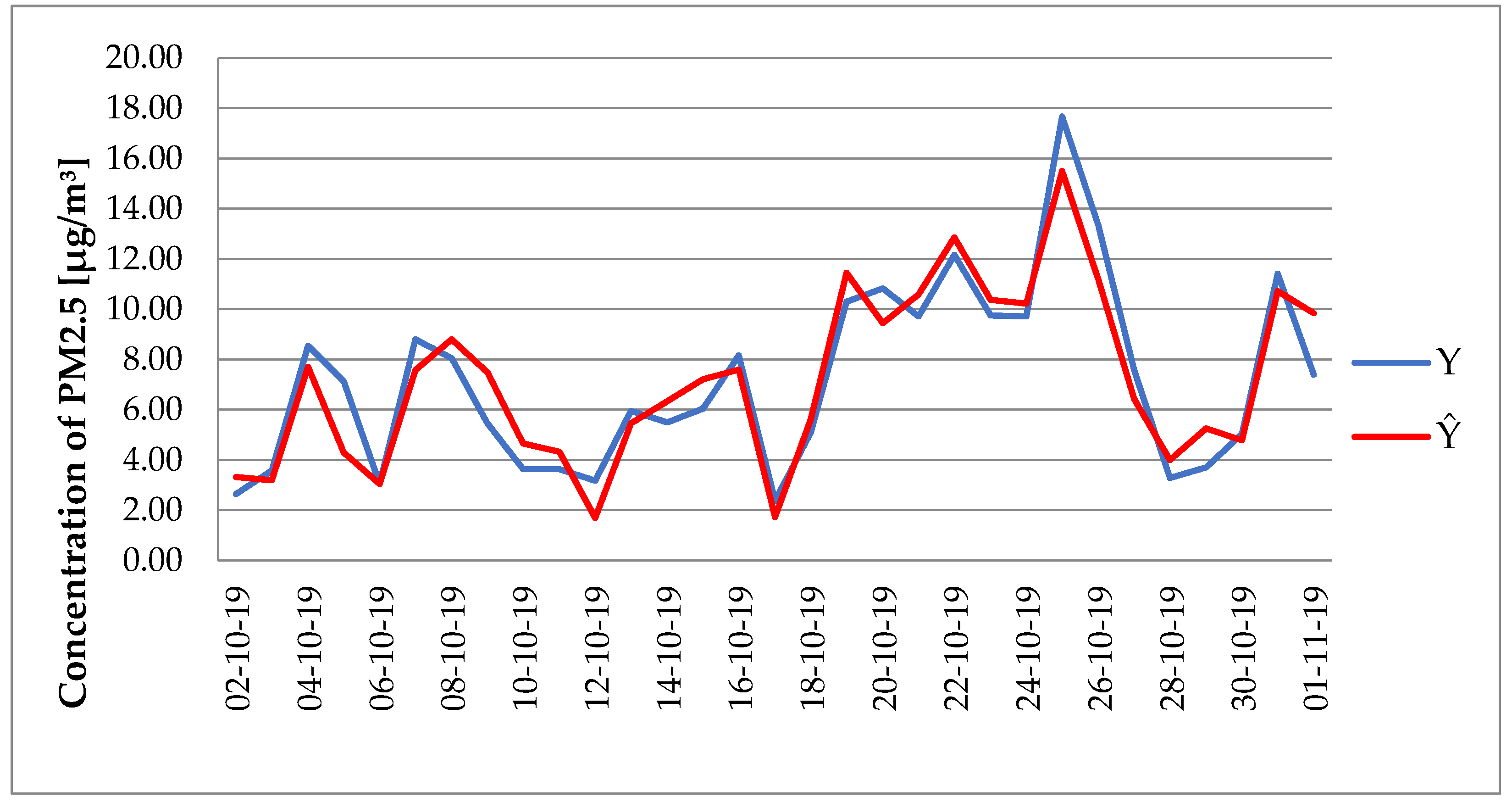
The graph representation of the actual concentration of PM2.5 in the room (Y) with the concentration calculated using the model () (Figure 5) illustrates the matching of the model with the real data. It can be stated that the degree of matching of the model with real data is high.
4. Conclusions
According to WHO Air Quality Guidelines recommendations, the concentration of PM10 should be below 50 μg/m3 per day and for PM2.5 below 25 μg/m3 per day in the outdoor and indoor environment [33]. The PM10 daily average concentration in the outdoor air was exceeded once during the period tested, while the PM2.5 daily outdoor average concentration exceeded the WHO recommended level for nine days. Increased levels of PM10 and PM2.5 particulates will without doubt adversely affect the air quality in the room. A linear regression model was built that allows estimation of PM2.5 concentration inside the building on the basis of data on atmospheric dust concentration. Statistical and substantive verification of the model indicates that the concentration of PM10 in outdoor air is the variable most strongly affecting the concentration of harmful PM2.5 in indoor air. The model therefore allows estimating the concentration of PM2.5 in the building on the basis of data on the concentration of PM10 outside the tested object, which can be useful for assessing indoor air quality without using a measuring tool inside the building.
Further research should consider including additional variables in the analysis, such as wind strength or vegetation covering the area. There is also a need to test the regression model in various environments, e.g., in a non-wooden building, in a multi-family building, in an office building. A tested and improved model can be a useful tool for determining indoor air quality in terms of PM2.5 concentration.
Author Contributions
Conceptualization: M.Z. and K.G.-F.; formal analysis: M.Z. and K.G.-F.; investigation: M.Z. and K.G.-F.; resources: M.Z. and K.G.-F.; writing—original draft preparation: M.Z.; writing—review and editing: M.Z.; project administration: M.Z.; funding acquisition: M.Z. All authors have read and agreed to the published version of the manuscript.
Funding
This research and APC was funded by the resources for young researchers WI/WB-IIŚ/13/2020 and WZ/WBiIS/4/2019 financed by the Ministry of Science and Higher Education of Poland.
Acknowledgments
Thanks to homeowners for providing space for measurements.
Conflicts of Interest
The authors declare no conflict of interest.
References
- Wysocka, M. DALY Indicator as an Assessment Tool for Indoor Air Quality Impact on Human Health. E3S Web Conf. 2018, 49, 00133. [Google Scholar] [CrossRef] [Green Version]
- Zabiegała, B. Indoor air quality—Volatile organic compounds as an indicator of indoor air quality. Monografie Komitetu Inżynierii Środowisko PAN 2009, 59, 303–315. [Google Scholar]
- Laska, M.; Dudkiewicz, E. Research of CO2 concentration in naturally ventilated lecture room. E3S Web Conf. 2017, 22, 00099. [Google Scholar] [CrossRef]
- Teleszewski, T.J.; Gładyszewska-Fiedoruk, K. Characteristics of humidity in classrooms with stack ventilation and development of calculation models of humidity based on the experiment. J. Build. Eng. 2020, 31, 101381. [Google Scholar] [CrossRef]
- Cong, X.; Zhao, J.; Jing, Z. Indoor particle dynamics in a school office: Determination of particle concentrations; deposition rates and penetration factors under naturally ventilated conditions. Environ. Geochem. Health 2018, 40, 2511–2524. [Google Scholar] [CrossRef]
- Nantka, M.B. Ventilation with Air Conditioning Elements; Silesian University of Technology Publisher: Gliwice, Poland, 2011. [Google Scholar]
- Kim, H.; Kang, K.; Kim, T. Measurement of Particulate Matter (PM2.5) and Health Risk Assessment of Cooking-Generated Particles in the Kitchen and Living Rooms of Apartment Houses. Sustainability 2018, 10, 843. [Google Scholar] [CrossRef] [Green Version]
- Wysocka, M. Analysis of indoor air quality in a naturally ventilated church. E3S Web Conf. 2018, 49, 00134. [Google Scholar] [CrossRef]
- Li, P.; Xin, J.; Wang, Y.; Li, G.; Pan, X.; Wang, S.; Cheng, M.; Wen, T.; Wang, G.; Liu, Z. Association between particulate matter and its chemical constituents of urban air pollution and daily mortality or morbidity in Beijing City. Environ. Sci. Pollut. Res. 2014, 22, 358–368. [Google Scholar] [CrossRef]
- Buonanno, G.; Giovinco, G.; Morawska, L.; Stabile, L. Lung cancer risk of airborne particles for Italian population. Environ. Res. 2015, 142, 443–451. [Google Scholar] [CrossRef] [Green Version]
- Czyżewski, B.; Matuszczak, A.; Kryszak, Ł.; Czyżewski, A. Efficiency of the EU Environmental Policy in Struggling with Fine Particulate Matter (PM2.5): How Agriculture Makes a Difference? Sustainability 2019, 11, 4984. [Google Scholar] [CrossRef] [Green Version]
- Bralewska, K.; Rogula-Kozłowska, W.; Bralewski, A. Size-Segregated Particulate Matter in a Selected Sports Facility in Poland. Sustainability 2019, 11, 6911. [Google Scholar] [CrossRef] [Green Version]
- Sobczak, P.; Mazur, J.; Zawiślak, K.; Panasiewicz, M.; Żukiewicz-Sobczak, W.; Królczyk, J.; Lechowski, J. Evaluation of Dust Concentration During Grinding Grain in Sustainable Agriculture. Sustainability 2019, 11, 4572. [Google Scholar] [CrossRef] [Green Version]
- Firląg, S.; Rogulski, M.; Badyda, A. The Influence of Marine Traffic on Particulate Matter (PM) Levels in the Region of Danish Straits. North and Baltic Seas. Sustainability 2018, 10, 4231. [Google Scholar] [CrossRef] [Green Version]
- European Environment Agency (EEA). Air Quality in Europe—2019 Report; Report No. 10/2019; EEA: Copenhagen, Denmark, 2019; Available online: https://www.eea.europa.eu//publications/air-quality-in-europe-2019 (accessed on 20 June 2020). [CrossRef]
- Majewski, G.; Rogula-Kozłowska, W.; Rozbicka, K.; Rogula-Kopiec, P.; Mathews, B.; Brandyk, A. Concentration, Chemical Composition and Origin of PM1: Results from the first long-term measurement campaign in Warsaw. Aerosol Air Qual. Res. 2018, 18, 636–654. [Google Scholar] [CrossRef]
- Juda-Rezler, K.; Toczko, B. Fine Dust in the Atmosphere. A Compendium of Knowledge about Air Pollution in Particulate Matter in Poland; Environmental Monitoring Library: Warsaw, Poland, 2016. [Google Scholar]
- Sówka, I.; Chlebowska-Stys, A.; Pachurka, Ł.; Rogula-Kozłowska, W.; Mathews, B. Analysis of particulate matter concentration variability and origin in selected urban areas in Poland. Sustainability 2019, 11, 5735. [Google Scholar] [CrossRef] [Green Version]
- Asikainen, A.; Carrer, P.; Kephalopoulos, S.; de Oliveira Fernandes, E.; Wargocki, P.; Hänninen, O. Reducing burden of disease from residential indoor air exposures in Europe (HEALTHVENT project). Environ. Health 2016, 15 (Suppl. 1), S35. [Google Scholar] [CrossRef]
- Asikainen, A.; Hänninen, O. Efficient Reduction of Indoor Exposures. Health Benefits from Optimizing Ventilation, Filtration and Indoor Source Controls. Report 2/2013 (National Institute of Health and Welfare. Tampere. 2013). Available online: http://www.julkari.fi/handle/10024/110211 (accessed on 8 February 2019).
- Yang, M.; Fan, H.; Zhao, K. PM2.5 Prediction with a Novel Multi-Step-Ahead Forecasting Model Based on Dynamic Wind Field Distance. Int. J. Environ. Res. Public Health 2019, 16, 4482. [Google Scholar] [CrossRef] [Green Version]
- Adães, J.; Pires, J.C.M. Analysis and Modelling of PM2.5 Temporal and Spatial Behaviors in European Cities. Sustainability 2019, 11, 6019. [Google Scholar] [CrossRef] [Green Version]
- Vicente, A.B.; Juan, P.; Meseguer, S.; Serra, L.; Trilles, S. Air Quality Trend of PM10. Statistical Models for Assessing the Air Quality Impact of Environmental Policies. Sustainability 2019, 11, 5857. [Google Scholar] [CrossRef] [Green Version]
- Załuska, M.; Gładyszewska-Fiedoruk, K. Analysis of PM10 and PM2.5 concentration in a single-family house. Rynek Instalacyjny 2019, 11, 52–55. [Google Scholar]
- Błaszczak, B.; Widziewicz-Rzońca, K.; Zioła, N.; Klejnowski, K.; Juda-Rezler, K. Chemical Characteristics of Fine Particulate Matter in Poland in Relation with Data from Selected Rural and Urban Background Stations in Europe. Appl. Sci. 2019, 9, 98. [Google Scholar] [CrossRef] [Green Version]
- Kowalska, M.; Skrzypek, M.; Kowalski, M.; Cyrys, J.; Ewa, N.; Czech, E. The Relationship between Daily Concentration of Fine Particulate Matter in Ambient Air and Exacerbation of Respiratory Diseases in Silesian Agglomeration. Poland. Int. J. Environ. Res. Public Health 2019, 16, 1131. [Google Scholar] [CrossRef] [PubMed] [Green Version]
- Rogulski, M. Low-cost PM monitors as an opportunity to increase the spatiotemporal resolution of measurements of air quality. Energy Procedia 2019, 128, 437–444. [Google Scholar] [CrossRef]
- Nidzgorska-Lencewicz, J. Application of Artificial Neural Networks in the Prediction of PM10 Levels in the Winter Months: A Case Study in the Tricity Agglomeration. Poland. Atmosphere 2018, 9, 203. [Google Scholar] [CrossRef] [Green Version]
- Adi Eko, T.P.; Wardoyo, A.Y. A model of particulate matter dispersion from unfiltered air conditioner indoor. J. Phys. Conf. Ser. 2019, 1153, 012107. [Google Scholar]
- Mei, X.; Gong, G. Influence of indoor air stability on suspended particle dispersion and deposition. Energy Procedia 2017, 105, 4229–4235. [Google Scholar] [CrossRef]
- Widder, S.H.; Haselbach, L. Relationship among Concentrations of Indoor Air Contaminants. Their Sources and Different Mitigation Strategies on Indoor Air Quality. Sustainability 2017, 9, 1149. [Google Scholar] [CrossRef] [Green Version]
- Zuśka, Z.; Kopcińska, J.; Dacewicz, E.; Skowera, B.; Wojkowski, J.; Ziernicka–Wojtaszek, A. Application of the Principal Component Analysis (PCA) Method to Assess the Impact of Meteorological Elements on Concentrations of Particulate Matter (PM10): A Case Study of the Mountain Valley (the Sącz Basin, Poland). Sustainability 2019, 11, 6740. [Google Scholar] [CrossRef] [Green Version]
- WHO Air Quality Guidelines for Particulate Matter, Ozone, Nitrogen Dioxide and Sulfur Dioxide. Summary of Risk Assessment. Available online: https://apps.who.int/iris/handle/10665/69477 (accessed on 15 May 2020).
- Urban PM2.5 Atlas: Air Quality in European Cities. Available online: https://ec.europa.eu/jrc/en/publication/eur-scientific-and-technical-research-reports/urban-pm25-atlas-air-quality-european-cities (accessed on 12 July 2020).
- PM10/PM2.5 Portable Particulate Monitor—Official Website of the Manufacturer of Measuring Devices Aeroqual. Available online: https://www.aeroqual.com/product/portable-particulate-monitor (accessed on 12 July 2020).
- Sobczyk, M. Statistics—Practical and Theoretical Aspects; Wydawnictwo Uniwersytetu Marii Skłodowskiej-Curie: Lublin, Poland, 2006. [Google Scholar]
- Gruszczyński, M.; Podgórska, M. Econometrics and Operational Research. In Handbook for Undergraduate Studies; Wydawnictwo Naukowe PWN: Warszawa, Poland, 2009. [Google Scholar]
- Qiu, L.; Liu, F.; Zhang, X.; Gao, T. Difference of Airborne Particulate Matter Concentration in Urban Space with Different Green Coverage Rates in Baoji, China. Int. J. Environ. Res. Public Health 2019, 16, 1465. [Google Scholar] [CrossRef] [Green Version]
- Cybulska, K.; Ciurzak, W.; Kowalski, P. Annual Air Quality Assessment in Podlaskie Voivodeship; Voivodship report for 2018; Chief Inspectorate for Environmental Protection, Department of Environmental Monitoring, Regional Department of Environmental Monitoring in Białystok: Białystok, Poland, 2019. [Google Scholar]
- Dahiru, T. p-value, a true test of statistical significance? A cautionary note. Ann. Ib Postgrad Med. 2008, 6, 21–26. [Google Scholar] [CrossRef] [Green Version]
Figure 1.
Airly sensor location on the map of Bialystok (Airly app view).

Figure 2.
Airly sensor location on the east wall of the building.

Figure 3.
Location of Airly sensor (1) and Aeroqual meter (2) in the room.

Figure 4.
Measuring station: 1—Airly sensor (outside, near the window), 2—Aeroqual sensor (inside, on the window sill).
Figure 4.
Measuring station: 1—Airly sensor (outside, near the window), 2—Aeroqual sensor (inside, on the window sill).

Figure 5.
Comparison of the actual PM2.5 concentration in the room (Y) with the concentration calculated using the model ().
Figure 5.
Comparison of the actual PM2.5 concentration in the room (Y) with the concentration calculated using the model ().


Table 1.
The average daily measurements of PM10 and PM2.5 concentration, temperature and relative air humidity.
Table 1.
The average daily measurements of PM10 and PM2.5 concentration, temperature and relative air humidity.
| PM2.5 INDOOR | PM10 OUTDOOR | PM2.5 OUTDOOR | Temperature OUTDOOR | Relative Humidity OUTDOOR | |
|---|---|---|---|---|---|
| µg/m3 | µg/m3 | µg/m3 | °C | % | |
| Day | Y | X1 | X2 | X3 | X4 |
| 2019-10-02 | 2.64 | 17.43 | 12.29 | 13.0 | 92.4 |
| 2019-10-03 | 3.58 | 17.04 | 11.67 | 8.3 | 81.9 |
| 2019-10-04 | 8.54 | 31.96 | 21.33 | 6.7 | 82.4 |
| 2019-10-05 | 7.13 | 20.63 | 13.96 | 6.0 | 82.7 |
| 2019-10-06 | 3.04 | 16.54 | 10.88 | 2.5 | 77.0 |
| 2019-10-07 | 8.79 | 31.54 | 20.96 | 2.4 | 81.4 |
| 2019-10-08 | 8.04 | 35.63 | 23.00 | 3.8 | 79.0 |
| 2019-10-09 | 5.46 | 31.25 | 20.54 | 9.5 | 86.5 |
| 2019-10-10 | 3.63 | 21.88 | 15.25 | 8.8 | 88.6 |
| 2019-10-11 | 3.63 | 20.79 | 14.42 | 8.7 | 83.5 |
| 2019-10-12 | 3.17 | 12.04 | 8.71 | 12.8 | 75.3 |
| 2019-10-13 | 5.96 | 24.54 | 17.04 | 13.7 | 85.1 |
| 2019-10-14 | 5.50 | 27.46 | 18.79 | 15.0 | 83.9 |
| 2019-10-15 | 6.04 | 30.33 | 20.50 | 15.0 | 82.5 |
| 2019-10-16 | 8.17 | 31.63 | 21.13 | 15.2 | 73.4 |
| 2019-10-17 | 2.38 | 12.17 | 8.92 | 11.8 | 77.9 |
| 2019-10-18 | 5.08 | 25.08 | 17.33 | 12.2 | 76.8 |
| 2019-10-19 | 10.29 | 44.38 | 29.92 | 12.5 | 82.5 |
| 2019-10-20 | 10.83 | 37.71 | 24.96 | 12.9 | 81.6 |
| 2019-10-21 | 9.71 | 41.54 | 28.21 | 13.9 | 80.2 |
| 2019-10-22 | 12.17 | 49.04 | 33.71 | 14.0 | 81.3 |
| 2019-10-23 | 9.75 | 40.83 | 28.13 | 11.3 | 83.3 |
| 2019-10-24 | 9.71 | 40.33 | 27.67 | 11.1 | 83.7 |
| 2019-10-25 | 17.67 | 57.79 | 40.38 | 11.5 | 90.3 |
| 2019-10-26 | 13.33 | 43.46 | 27.75 | 11.4 | 82.9 |
| 2019-10-27 | 7.58 | 27.75 | 18.29 | 11.8 | 75.6 |
| 2019-10-28 | 3.29 | 19.71 | 13.38 | 6.5 | 75.8 |
| 2019-10-29 | 3.71 | 23.88 | 16.13 | 4.8 | 78.7 |
| 2019-10-30 | 5.04 | 22.29 | 15.00 | 2.0 | 78.3 |
| 2019-10-31 | 11.42 | 41.96 | 26.67 | 1.3 | 78.2 |
| 2019-11-01 | 7.40 | 39.05 | 25.10 | 2.2 | 78.2 |
Table 2.
Summary of statistical parameters of independent variables.
| PM10 OUTDOOR | PM2.5 OUTDOOR | Temperature OUTDOOR | Relative Humidity OUTDOOR | |
|---|---|---|---|---|
| µg/m3 | µg/m3 | °C | % | |
| X1 | X2 | X3 | X4 | |
| Average (-) | 30.25 | 20.39 | 9.43 | 81.31 |
| Standard deviation (-) | 11.34 | 7.56 | 4.42 | 4.41 |
| Variability coefficient (%) | 37.50 | 37.08 | 46.85 | 5.42 |
Table 3.
The selection of independent variables using the Hellwig method.
| PM10 OUTDOOR | PM2.5 OUTDOOR | Temperature OUTDOOR | |
|---|---|---|---|
| X1 | X2 | X3 | |
| C1 | 1 | 0 | 0 |
| C2 | 0 | 1 | 0 |
| C3 | 0 | 0 | 1 |
| C4 | 1 | 1 | 0 |
| C5 | 0 | 1 | 1 |
| C6 | 1 | 0 | 1 |
| C7 | 1 | 1 | 1 |
Table 4.
Correlation matrix.
| PM2.5 INDOOR | PM10 OUTDOOR | PM2.5 OUTDOOR | Temperature OUTDOOR | |
|---|---|---|---|---|
| Y | X1 | X2 | X3 | |
| Y | 1 | 0.93791953 | 0.93476573 | 0.1306016 |
| X1 | 0.93791953 | 1 | 0.99613666 | 0.1297334 |
| X2 | 0.93476573 | 0.99613666 | 1 | 0.1749146 |
| X3 | 0.13060164 | 0.12973339 | 0.1749146 | 1 |
Table 5.
Capacity (H) of each combination of variable.
| PM10 OUTDOOR | PM2.5 OUTDOOR | Temperature OUTDOOR | Information capacity | |
|---|---|---|---|---|
| X1 | X2 | X3 | H | |
| C1 | 0.879693 | 0 | 0 | 0.879693 |
| C2 | 0 | 0.873787 | 0 | 0.873787 |
| C3 | 0 | 0 | 0.017057 | 0.017057 |
| C4 | 0.440698 | 0.437739 | 0 | 0.878437 |
| C5 | 0 | 0.743703 | 0.014517 | 0.758220 |
| C6 | 0.778673 | 0 | 0.015098 | 0.793771 |
| C7 | 0.413804 | 0.402472 | 0.013073 | 0.829349 |
Combination C1 (X1) shows the greatest information capacity.
Table 6.
Regression statistics.
| Statistics of Regression | |
|---|---|
| R multiple | 0.93791953 |
| R square | 0.87969305 |
| Fitting R square | 0.87554453 |
| Standard error | 1.28702562 |
| Observations | 31 |
Table 7.
Analysis of variance.
| Variance Analysis | |||||
|---|---|---|---|---|---|
| df | SS | MS | F | Significance F | |
| Regression | 1 | 351.24715 | 351.24715 | 21.05007 | 7.197 × 10⁻¹⁵ |
| Residual | 29 | 48.0366136 | 1.65643495 | ||
| Total | 30 | 399.283764 | |||
Table 8.
Directional coefficients.
| Coefficients | Standard Error | t-Stat | p-Value | Bottom 95% | Peak 95% | |
|---|---|---|---|---|---|---|
| Intersection | −1.942038 | 0.667901 | −2.907673 | 0.006914 | −3.308049 | −0.576027 |
| X1 | 0.301682 | 0.020717 | 14.561939 | 7.197 × 10⁻¹⁵ | 0.259311 | 0.344054 |
© 2020 by the authors. Licensee MDPI, Basel, Switzerland. This article is an open access article distributed under the terms and conditions of the Creative Commons Attribution (CC BY) license (http://creativecommons.org/licenses/by/4.0/).
Share and Cite
MDPI and ACS Style
Załuska, M.; Gładyszewska-Fiedoruk, K. Regression Model of PM2.5 Concentration in a Single-Family House. Sustainability 2020, 12, 5952. https://0-doi-org.brum.beds.ac.uk/10.3390/su12155952
AMA Style
Załuska M, Gładyszewska-Fiedoruk K. Regression Model of PM2.5 Concentration in a Single-Family House. Sustainability. 2020; 12(15):5952. https://0-doi-org.brum.beds.ac.uk/10.3390/su12155952
Chicago/Turabian StyleZałuska, Monika, and Katarzyna Gładyszewska-Fiedoruk. 2020. "Regression Model of PM2.5 Concentration in a Single-Family House" Sustainability 12, no. 15: 5952. https://0-doi-org.brum.beds.ac.uk/10.3390/su12155952
Note that from the first issue of 2016, this journal uses article numbers instead of page numbers. See further details here.