The Optimal Allocation and Operation of an Energy Storage System with High Penetration Grid-Connected Photovoltaic Systems

Abstract

High-penetration grid-connected photovoltaic (PV) systems can lead to reverse power flow, which can cause adverse effects, such as voltage over-limits and increased power loss, and affect the safety, reliability and economic operations of the distribution network. Reasonable energy storage optimization allocation and operation can effectively mitigate these disadvantages. In this paper, the optimal location, capacity and charge/discharge strategy of the energy storage system were simultaneously performed based on two objective functions that include voltage deviations and active power loss. The membership function and weighting method were used to combine the two objectives into a single objective. An energy storage optimization model for a distribution network considering PV and load power temporal changes was thus established, and the improved particle swarm optimization algorithm was utilized to solve the problem. Taking the Institute of Electrical and Electronic Engineers (IEEE)-33 bus system as an example, the optimal allocation and operation of the energy storage system was realized for the access of high penetration single-point and multi-point PV systems in the distribution network. The results of the power flow optimization in different scenarios were compared. The results show that using the proposed approach can improve the voltage quality, reduce the power loss, and reduce and smooth the transmission power of the upper-level grid.

1. Introduction

In the context of the rapid development of the global economy, the continuous growth of energy demands, the gradual depletion of fossil fuels and the increasing environmental pressure, many countries and regions are vigorously advocating for the reform and transformation of current energy structures, and have introduced various policies to promote the use and development of clean energy. Photovoltaic (PV) power generation technology has been rapidly developed and applied during this period [1,2,3]. With the increasing penetration rate and number of distributed PVs in the distribution network, adverse effects such as power backflows, the bus voltage being out of limit, power loss increases, harmonic increases and power supply reliability reductions may occur [4,5]. At the same time, the PV power output varies over time due to intermittency, randomness and volatility. The load changes also have time sequence characteristics, and the peak and valley of the PV power output and those of the load in the distribution network are not completely matched [6]. The double uncertainty of renewable energy and load leads to greater uncertainty regarding the power flow in the grid, which restricts the consumption of PV power in the distribution network. An energy storage system with a rapid energy response ability can, to a certain extent, ease PV grid power, shift the peak load, decrease the power loss, improve the voltage quality, reduce the injected power of the upper-level grid, improve the system stability, and optimize the operations of the distribution network, which involves the flexible scheduling of load side resources and an effective means of achieving demand-side management [7,8,9,10]. On the other hand, the energy storage system is a solution to increase the share of self-consumption in a developed market which is conducive to the economic feasibility of PV systems, and it can lead to less pollution of the environment and lower carbon dioxide (CO₂) emissions [11,12]. Therefore, under the conditions of a high penetration multi-access point grid-connected PV, it is important to achieve optimal allocation and operational planning for energy storage systems to optimize the power flow of the grid, improve the absorption capacity and peak-cutting benefit of PV power in the distribution network, and promote the safety, stability and economic operations of the power system [13,14].

Many scholars have studied the optimal allocation and operation of distributed energy storage in a distribution network. Kabir et al. [15] determined the capacity of an energy storage system to solve the problem of the overvoltage produced by high penetration grid-connected PVs and the lower voltage brought by the peak load. Bennett et al. [16] optimized the capacity and the charging and discharging operational strategy of a battery energy storage system to achieve the load balancing, peak and valley filling, and rooftop PV optimization management in a low-voltage distribution network. The authors of [15,16] optimized the capacity of energy storage, but the locations of energy storage were given in advance, and the optimal location was not selected. Sardi et al. [17] determined the location and capacity of energy storage to maximize the net present value and increase the load factor and voltage level based on a cost–benefit analysis. Hashemi et al. [18] calculated the minimum energy storage capacity at different locations based on the voltage sensitivity analysis method to avoid overvoltage under the conditions of a high penetration grid-connected PV system. Yuan et al. [19] used the minimum power loss as their optimization objective, and applied the Coyote optimization algorithm to solve and obtain the optimal location and capacity of a lithium-ion battery energy storage system. Tang and Low [20] determined the optimal location and capacity of energy storage in a distribution network based on the continuous tree theory of the linear discrete flow model to minimize the total active power loss of the system. Giannitrapani et al. [21] determined the location and quantity of energy storage systems according to voltage sensitivity, determined the capacity of energy storage based on the multi-stage power flow, and then determined the optimal installation location, quantity, and capacity of energy storage systems in a low-voltage distribution network with the minimum total cost as the optimization objective. Das et al. [22] used the voltage deviation, flicker, power loss and line loading as the optimization objectives, and utilized a fitness-scaled chaotic artificial bee colony algorithm to solve the objective function to achieve the optimal configuration of the energy storage system. Wong et al. [23] used the minimum active power loss of the distribution network as their optimization objective, and applied the whale optimization algorithm to obtain the optimal location and capacity of energy storage. The optimization process was carried out by first optimizing the position and then optimizing the capacity, while simultaneously optimizing the position and the capacity. The results obtained were compared with the results from using the firefly algorithm and particle swarm optimization algorithm, thus verifying the superiority of the proposed algorithm. In the literature [17,18,19,20,21,22,23], the location and capacity of the energy storage were optimized, but the optimal operation of energy storage charging and discharging was not considered. Reihani and Ghorbani [24] controlled the optimal charging and discharging operations of energy storage by load power predictions to achieve peak adjustment and power leveling with the access of high penetration and multi-point PV systems to the distribution network. Nagarajan and Ayyanar [25] used the convex optimization method to optimize the charging and discharging strategy of a Li-ion battery energy storage system to reduce the impact of intermittent PV power generation on the system. In the literature [24,25], a charging and discharging operational strategy optimization for energy storage was realized, but this study was carried out under the premise that the location and capacity of the energy storage are pre-established. Mahani et al. [26] optimized the planning and operation of the energy storage location and capacity in the distribution network with a high penetration rate of renewable energy to realize the peak adjustment and reduce the reverse power flow and price arbitrage. Grisales-Noreña et al. [27] selected the minimum energy loss as the optimization objective, and used a master–slave strategy to solve the problem to obtain the optimal position and the charge/discharge operational control strategies for energy storage batteries and capacitors banks. In the literature [26,27], the voltage regulation of a distribution network before and after the configuration of the energy storage system was not considered.

To our knowledge, there are few studies on energy storage optimization allocation and operation that simultaneously consider the joint optimization of the installation location, capacity, charge/discharge power of an energy storage system, and power flow. Usually, the studies are only part of them, while other factors are given in advance. In addition, in the present study, the location of the PV system in the power grid is composed of one point or several points, and multi-point cases are not considered.

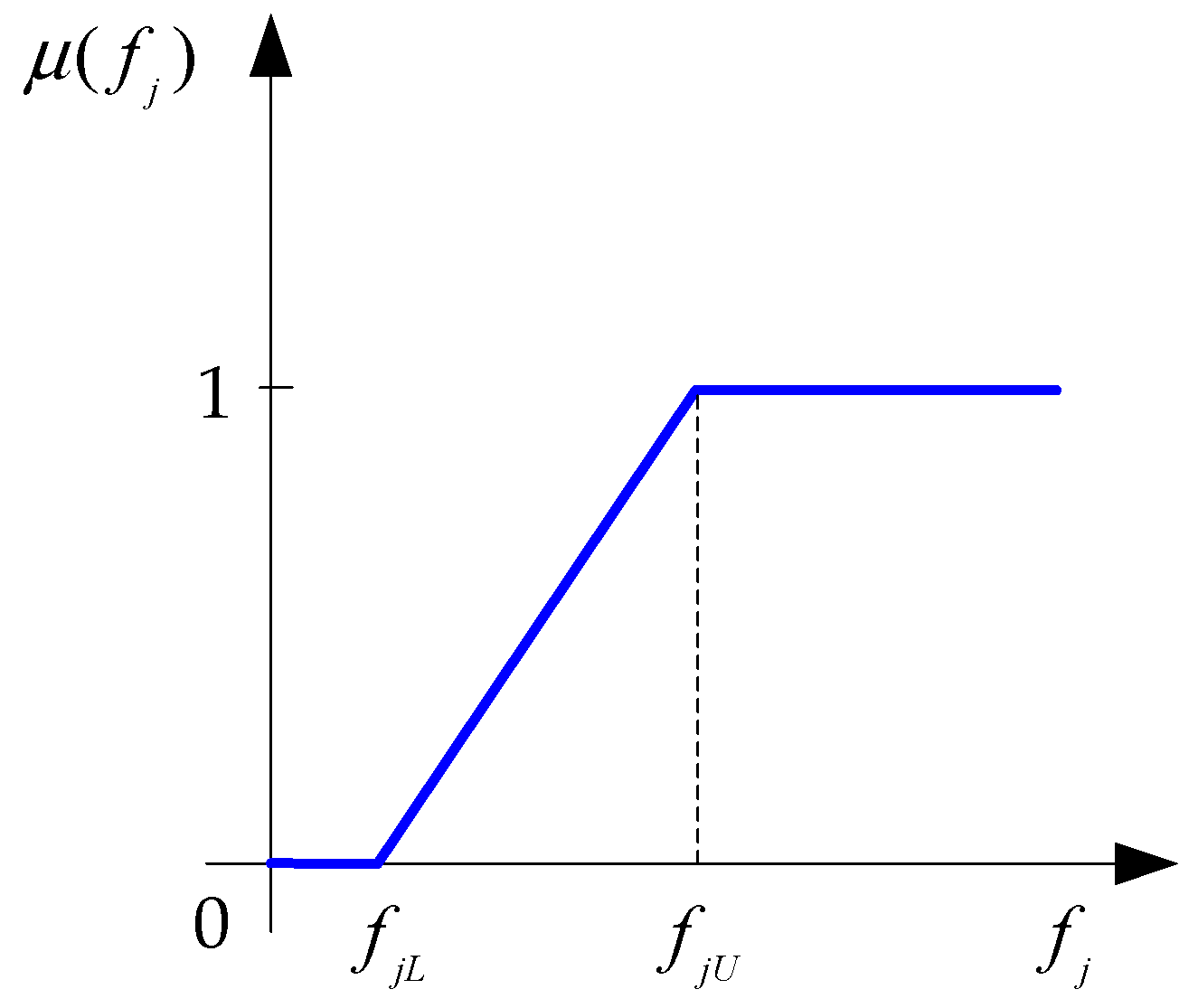
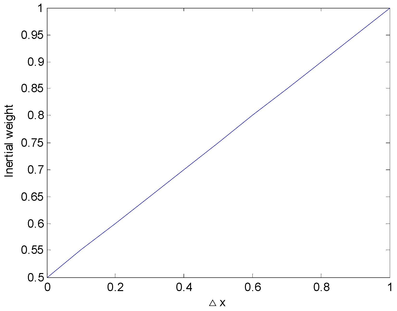
The objective of the paper is to propose a new optimization approach that used an improved particle swarm optimization algorithm to determine the energy storage systems’ locations, capacities and charge/discharge strategy simultaneously to minimize the voltage deviations and total active power loss for the access of high penetration single-point and multi-point PV systems in the distribution network. The membership function and weighting method are used to combine the two objectives into a single objective. The differential inertial weights and global guided cross search mechanism are utilized in the improved algorithm. The Institute of Electrical and Electronic Engineers (IEEE)-33 bus feeder system is examined. The power flow optimization results under different scenarios in the distribution network are achieved to verify its efficiency.

2. Mathematical Model of the Optimal Allocation and Operation for an Energy Storage System

In order to optimize the power flow of the distribution network with PV systems, the optimization objectives are to minimize the bus voltage deviation and active power loss; the power balance, bus voltage, energy storage power, charge/discharge balance and remaining capacity of the energy storage system are the constraints. The optimal location and capacity of the energy storage system are determined by the improved particle swarm optimization algorithm.

2.1. The Objective Function

2.1.1. Objective 1: The Minimization of Bus Voltage Deviations

Voltage stability is one of the main purposes of power flow optimization. It is of great significance for the safe and stable operation of the distribution network to maintain the voltage of each bus at a certain level in the network. PV power generation has randomness and volatility. Although PV power under certain penetration rates improves the voltage quality to some extent, it also aggravates the deviation of the bus voltage. Therefore, the sum of the voltage deviations of all buses in the distribution network for one day was taken as the objective function of the optimal energy storage allocation, as shown in (1).

$$f_1={\displaystyle \sum {}_{i=1}^N}{\displaystyle \sum {}_{t=1}^T}|U_{i,t}-U_N|,$$

(1)

where N is the total number of buses in the distribution network, and T is the total number of selected moments in this research, T = 24. $U_{i,t}$ is the voltage amplitude of bus i at t, and $U_N$ is the rated voltage of the distribution network.

2.1.2. Objective 2: The Minimization of Active Power Loss

The average value of active power loss during the study period was selected as the objective function of optimization, as shown in (2).

$$f_2=\frac{{\displaystyle \sum {}_{t=1}^T}{P}_{t,\mathrm{L}}}{T},$$

(2)

where $P_{t,\mathrm{L}}$ is the active power loss at time t. The calculation method is the same as that in [28].

2.1.3. The Double Objectives Become a Single Objective

In this paper, our objective is that the voltage deviation of each bus and the power loss of the grid be as small as possible, so it is necessary to consider objective 1 and objective 2 at the same time. Since the dimensions of objective 1 and objective 2 are different, they cannot be added directly. Therefore, this paper will use the membership function of fuzzy mathematics to calculate the membership degree of each objective [29], then the weighted method will be used to transform objective 1 and objective 2 into a single objective. The general idea is: first, the optimal solution of each single objective under all constraints is obtained, and then the membership degree of each objective is calculated according to the membership function, and then the memberships are added linearly. Finally, the multi-objective optimization problem is transformed into a single objective optimization problem. According to the above method, the problems of the different dimensions for objective 1 and objective 2 are solved at the same time. The steps are as follows:

In the first step, the optimal solution of objective 1 under the constraint condition is first obtained; that is, the minimum value of the voltage deviation is obtained as the lower limit of voltage deviation $f_{1\mathrm{L}}$. At the same time, the value of objective 2, active power loss, is calculated as the upper limit of power loss $f_{2\mathrm{U}}$.

In the second step, the optimal solution of objective 2 under the constraint conditions, the minimum value of active power loss, is obtained as the lower limit of active power loss $f_{2\mathrm{L}}$. At the same time, the value of objective 1, the value of voltage deviation, is calculated as the upper limit of voltage deviation $f_{1\mathrm{U}}$.

In the third step, fuzzy processing is carried out for the objective function, and an ascending half trapezoid distribution is selected for the membership function, as shown in (3). The distribution is shown in Figure 1.

$$\mu (f_j)=\{\begin{array}{c}0\begin{array}{ccc}& & f_j<f_{j\mathrm{L}}\end{array}\\ \frac{f_j-f_{j\mathrm{L}}}{f_{j\mathrm{U}}-f_{j\mathrm{L}}}\begin{array}{ccc}& f_{j\mathrm{L}}<f_j<f_{j\mathrm{U}}& \end{array}\\ 1\begin{array}{ccc}& & f_j>f_{j\mathrm{U}}\end{array}\end{array},$$

(3)

where $\mu (f_j)$ is the membership of the objective function j.

The membership of objective function (1) and (2) is then linearly weighted to obtain the single objective function as follows:

$$\min \left\{\alpha \cdot \mu (f_1)+\beta \cdot \mu (f_2)\right\}$$

(4)

where $\alpha$ and $\beta$ are the weight coefficients of $\mu (f_1)$ and $\mu (f_2)$, respectively, where $\alpha +\beta =1$. The weight coefficient reflects the relative importance of each sub-objective. In this paper, $\alpha =\beta =0.5$.

2.2. Constraint Condition

2.2.1. Power Balance Constraints

$$P_{sum}+{\displaystyle \sum {}_{j=1}^m}{P}_{c,j}+{\displaystyle \sum {}_{k=1}^n}{P}_{g,k}={\displaystyle \sum {}_{i=1}^N{P}_{l,i}},$$

(5)

where $P_{sum}$ is the active power injected into the distribution network from the upper-level grid; m is the number of energy storage systems; $P_{c,j}$ is the power of the j-th energy storage system, where the specified positive value is the discharge; n is the number of grid-connected PV systems; $P_{g,k}$ is the power of the k-th PV systems; N is the number of buses in the distribution network; and $P_{l,i}$ is the load power of bus i.

2.2.2. Bus Voltage Constraints

$$U_{\min }<U_{i,j}<U_{\max }$$

(6)

where $U_{\min }$ is the minimum value of the specified bus voltage, which is 0.95 $U_N$; $U_{\max }$ is the maximum bus voltage, which is 1.05 $U_N$; and $U_{i,j}$ is the voltage value of bus i at time j.

2.2.3. Power Constraints of the Energy Storage System

$$P_{c,\min }<P_{c,j}<P_{c,\max }$$

(7)

where $P_{c,\min }$ is the minimum power of the energy storage system; $P_{c,\max }$ is the maximum power of the energy storage system; and $P_{c,j}$ is the power of the energy storage system at j moment.

2.2.4. Charge/Discharge Balance Constraints of the Energy Storage Systems

$${\displaystyle \sum {}_{t=1}^T}{P}_{c,t}\ast \Delta t=0$$

(8)

where $P_{c,t}$ is the power of the energy storage system at moment t, and $\Delta t$ is the time interval between two moments.

2.2.5. The Remaining Power Constraints of the Energy Storage System

$$E_{c\min }\le E_{ct}\le E_{c\max }$$

(9)

where $E_{ct}$ is the remaining power of the energy storage unit at moment t, and $E_{c\max }$ and $E_{c\min }$ are the upper and lower limits of the remaining capacity of the energy storage system, which are 0.9 and 0.2 times the rated capacity of the energy storage system, respectively. That is, the state of charge (SOC) values of the energy storage system range from 20% to 90%.

3. Solving Algorithm

In the particle swarm optimization (PSO) algorithm, the particles update their speed and position by tracking their own historical optimal solution and the global optimal solution of the population. The update method is shown in (10) and (11) [30].

$$v_{id}^{\left(k+1\right)}=w{v}_{id}^{\left(k\right)}+c_1{r}_1\left(p_{id}^{\left(k\right)}-x_{id}^{\left(k\right)}\right)+c_2{r}_2\left(p_{gd}^{\left(k\right)}-x_{id}^{\left(k\right)}\right),$$

(10)

$$x_{id}^{\left(k+1\right)}=x_{id}^{\left(k\right)}+v_{id}^{\left(k+1\right)},$$

(11)

where w is the inertial weight, c₁ and c₂ are the acceleration factors, and r₁ and r₂ are random numbers between 0 and 1; $p_{id}^{\left(k\right)}$ is the d-dimensional component of the i-th particle in the optimal position vector of the k-th iteration, and $p_{gd}^{\left(k\right)}$ is the d-dimensional component of the optimal position vector of the k-th iteration population.

In order to solve the problem of the fixed inertial weights and make it easy to fall into a local optimal solution in the iteration process of a conventional PSO algorithm, an improved PSO algorithm is proposed in this paper.

3.1. Improved Particle Swarm Optimization Algorithm

3.1.1. Differential Inertial Weight

The balance between the exploration ability and development ability of the intelligent optimization method is the key to its successful operation, and a reasonable value of inertial weight $\omega$ is an important way to achieve balance between these two capabilities in the PSO algorithm. In the PSO algorithm, the value of inertial weight $\omega$ has different forms, such as fixed weight, which is a better value obtained from experience; time-varying weight, which decreases as the number of iterations increases; fuzzy weight; which is a kind of dynamic adjustment based on fuzzy systems; and random weight, which is a random value in a certain range [31]. However, none of these inertial weights take into account the characteristics of the particles in the iteration process.

The difference between the position of a particle and the corresponding position of the global optimum particle of the population reflects the difference between the current solution and the optimum solution. Thus, increasing the value of $\omega$ when the difference is large can increase the flight speed and improve the global search ability of the particle. When the difference is small, reducing the value of $\omega$ can reduce the flight speed and improve the particle’s local search ability. In the improved particle swarm optimization (IPSO) of this paper, the size of $\omega$ is linearly adjusted according to the difference between the position of the particle and the corresponding variable of the optimal particle position of the population.

The difference between the position of the i-th particle in the k-th iteration and the global optimal position of the population is shown in (12). The inertial weight of the i-th particle in the update speed of its position in the k-th iteration is defined as the differential inertial weight, as shown in (13).

$$\Delta x_i^{(k)}=\frac{1}{x_{\max }-x_{\min }}\frac{1}{D}{\displaystyle \sum _{d=1}^D|p_{gd}^{(k)}}-x_{id}^{(k)}|,$$

(12)

$${\omega }_i^{\left(k\right)}={\omega }_{\max }-({\omega }_{\max }-{\omega }_{\min }\left)\right(1-\Delta x_i^{(k)}),$$

(13)

where $x_{\max }$ and $x_{\min }$ are the maximum and minimum values of the particle position variables, respectively and ${\omega }_{\max }$ and ${\omega }_{\min }$ are the maximum and minimum inertial weights, respectively.

The differential inertial weight curve when the maximum inertial weight ${\omega }_{\max }$ is set to 1 and ${\omega }_{\min }$ is set to 0.5 is shown in Figure 2.

3.1.2. Global Guided Cross-Search Mechanism

Because PSO is prone to falling into a local optimal solution during its iterations, a global guided cross-search mechanism to update the location of the particles is introduced [32] using (14). Guiding the new solution to a global optimal solution improves the convergence speed of the algorithm:

$$X_{id}^{(k)}={\{}_{P_{gd}^{(k)}+b{(P_{gd}^{(k)}-X_{id}^{(k)})}_{}\hspace{1em}otherwise}^{X_{id}^{(k)}\hspace{1em}\hspace{1em}\hspace{1em}rand<cr},$$

(14)

where rand is the random value of the uniform distribution between 0 and 1, and b is a random value between −1 and 1. Increasing the value of the coefficient cr is conducive to enhancing the development ability of the algorithm, while reducing the value of the coefficient cr is beneficial to the search ability of the algorithm. In this paper, cr is 0.6 [28].

3.1.3. Coding Method

Because the charging and discharging power of the energy storage system at each moment is affected by the load change, the PV power output and the charge/discharge of the energy storage system have constraints. In the optimization process, the installation location of the energy storage system and the charging or discharging power at each moment are taken as the optimization variables, and the coding method is as follows.

The position x of each particle in the solution process is the variable to be optimized, as shown in (15), including the installation location and the charging or discharging power at each time of the energy storage system in the distribution network; each particle is a (m + 1) *T-dimensional vector.

$$x=(x_l,x_p)$$

(15)

$$x_l=(x_{l1},x_{l2}\dots x_{lj}\dots x_{lm})$$

(16)

$$x_p=(x_{p1+1},x_{p1+2},\dots x_{p1+T},x_{p2+1},x_{p2+2},\dots x_{p2+T},\dots x_{pj+t}\dots x_{pj+T})$$

(17)

where $x_{lj}$ is the position variable of the j-th energy storage system, which is an integer; $x_{pj+t}$ is the charging or discharging power of the j-th energy storage system at moment t; m is the number of energy storage systems in the distribution network; and T is the total number of moments.

In this case, the differential inertial weight in the update speed of the different location variables for each particle is calculated as follows:

$$\Delta x_{li}^{(k)}=\frac{1}{x_{l\max }-x_{l\min }}\frac{1}{m}{\displaystyle \sum _{d=1}^m|p_{gd}^{(k)}}-x_{id}^{(k)}|,$$

(18)

$${\omega }_{li}^{(k)}={\omega }_{\max }-({\omega }_{\max }-{\omega }_{\min })(1-\Delta x_{li}^{(k)}),$$

(19)

$$\Delta x_{pi}^{(k)}=\frac{1}{x_{p\max }-x_{p\min }}\frac{1}{mT}{\displaystyle \sum _{d=m+1}^{(m+1)T}|p_{gd}^{(k)}}-x_{id}^{(k)}|,$$

(20)

$${\omega }_{pi}^{(k)}={\omega }_{\max }-({\omega }_{\max }-{\omega }_{\min })(1-\Delta x_{pi}^{(k)}),$$

(21)

where $\Delta x_{li}^{(k)}$ is the difference between the position variable of the energy storage system and the global optimal position of the population for the i-th particle in k iterations; ${\omega }_{li}^{(k)}$ is the differential inertial weight of the i-th particle in the update speed of the energy storage system position variable in k iterations; $\Delta x_{pi}^{(k)}$ is the difference between the power variable of the energy storage system and the global optimal position of the population for the i-th particle in k iterations; and ${\omega }_{pi}^{(k)}$ is the differential inertial weight in the update speed of the power variable of the storage system for the i-th particle in k iterations.

$x_{l\max }$ and $x_{l\min }$ are the maximum and minimum values of the location variables of the energy storage system, respectively.

$x_{p\max }$ and $x_{p\min }$ are the maximum and minimum power variables of the energy storage system, respectively.

3.2. Solution Steps

Step 1: read the network data. Read the parameters of the distribution network to be optimized, the locations of the grid-connected PV systems, the load demand and the PV power output data at each moment, etc.

Step 2: initialize the parameters of the IPSO. Create the initialization conditions, determine the total number of particles N, the particle dimensions D, the number of iterations k = 1, and the maximum number of iterations MaxDT, as well as the size of parameters ${\omega }_{\max }, {\omega }_{\min }$, c₁, c₂, r₁ and r₂.

Step 3: initialize the particles. According to the coding method shown in (15)–(17), the energy storage position variable uses integer encoding, the energy storage power variable uses real encoding, and the particle position x_i and velocity v_i are randomly generated within the constraint range of the network parameters. The particle position vector includes the installation position variable of the energy storage system and the charging or discharging power variable of the energy storage at each moment. Correspondingly, the particle velocity vector includes the velocity of the energy storage system position variable (which should be an integer) and the velocity of the energy storage system power.

Step 4: call the power flow program to calculate the value of objective function (1) and objective function (2), thereby satisfying the constraint conditions. According to the fuzzification method mentioned in Section 2.1, the double objectives are changed into a single objective. The return value is the initial fitness of each particle, which is the current optimal value of the particle. The current global optimal value is obtained by sorting and comparing the current optimal value of each particle. The particle whose objective function value is equal to the global optimal value is the global optimal particle. Set iteration number k = 1.

Step 5: enter the main cycle. According to (18)–(21), calculate the differential inertial weight of the energy storage position variable and the power variable in each iteration; then, calculate the new position and velocity variables of the particles in each iteration according to (10) and (11). The position and velocity variables of the particles are updated according to the global guided cross mutation operation, as shown in (14). Next, call the power flow calculation program, calculate and compare, update the optimal fitness and global optimal fitness of each particle, and record the corresponding positions of the particles.

Step 6: the convergence judgment. If the iteration number k reaches the maximum iteration number MaxDT, the iteration ends, and the optimal solution is output; otherwise, k = k + 1, and the loop command continues to be executed in step 4.

The calculation flow chart is shown in Figure 3.

4. Results and Discussion

The IEEE-33 bus radial distribution system was examined to test the validity of the optimization ideas proposed in this paper. The distribution network diagram is shown in Figure 4. Bus 1 is the balanced bus, and is also the bus connected to the upper-level power grid. The voltage amplitude of bus 1 is 12.66 kV, the nominal value is 1.0 p.u., and the phase angle is 0. The allowable voltage deviation range of each bus in the distribution network in this area is ±5% U_N, the total active power load is 3715 kW, and the total reactive power load is 2300 kvar. The total active power loss is 202.6878 kW, and the total reactive power loss is 135.6112 kvar without grid-connected PV systems. The typical daily load curve of the distribution network is shown in Figure 5. The data in Figure 5 is from reference [33], as shown in

Table A1. The data of Figure 5.

Time (h)	Active Power (kW)	Time (h)	Active Power (Kw)
0:00	2950	12:00	3500
1:00	2800	13:00	3350
2:00	2650	14:00	3250
3:00	2500	15:00	3150
4:00	2450	16:00	3150
5:00	2400	17:00	3300
6:00	2450	18:00	3700
7:00	2550	19:00	3715
8:00	2650	20:00	3650
9:00	3000	21:00	3600
10:00	3300	22:00	3400
11:00	3450	23:00	3200

of Appendix A, which shows the total active power load of all of the buses (except bus 1) in the IEEE-33 bus system at each time, and the maximum active power load is 3715kW. The line and load data of the IEEE-33 bus system are shown in

Table A2. Line and load data of the IEEE-33 bus system.

Line No.	Start Bus	End Bus	Line Resistance (Ω)	Line Reactance (Ω)	Active Power Load (kW)	Reactive Power Load (kvar)
1	1	2	0.0922	0.047	100	60
2	2	3	0.493	0.2511	90	40
3	3	4	0.366	0.1864	120	80
4	4	5	0.3811	0.1941	60	30
5	5	6	0.819	0.707	60	20
6	6	7	0.1872	0.6188	200	100
7	7	8	0.7114	0.2351	200	100
8	8	9	1.03	0.74	60	20
9	9	10	1.044	0.74	60	20
10	10	11	0.1966	0.065	45	30
11	11	12	0.3744	0.1238	60	35
12	12	13	1.468	1.155	60	35
13	13	14	0.5416	0.7129	120	80
14	14	15	0.591	0.526	60	10
15	15	16	0.7463	0.545	60	20
16	16	17	1.289	1.721	60	20
17	17	18	0.732	0.574	90	40
18	2	19	0.164	0.1565	90	40
19	19	20	1.5042	1.3554	90	40
20	20	21	0.4095	0.4784	90	40
21	21	22	0.7089	0.9373	90	40
22	3	23	0.4512	0.3083	90	50
23	23	24	0.898	0.7901	420	200
24	24	25	0.896	0.7011	420	200
25	6	26	0.203	0.1034	60	25
26	26	27	0.2842	0.1447	60	25
27	27	28	1.059	0.9337	60	20
28	28	29	0.8042	0.7006	120	70
29	29	30	0.5075	0.2585	200	600
30	30	31	0.9744	0.963	150	70
31	31	32	0.3105	0.3619	210	100
32	32	33	0.341	0.5302	60	40

of Appendix A. In the IEEE-33 bus system, the active power load of each bus is considered to be the maximum active power of the corresponding bus. The active power changes of each bus at different times are considered to be consistent with the time series changing trend of a typical daily load curve (Figure 5). The active power load of each bus at each time in the distribution network is shown in Figure 6. The data of Figure 6 is shown in

Table A3. The data of Figure 6 (kW).

Bus	Time (h)
	0:00	1:00	2:00	3:00	4:00	5:00	6:00	7:00	8:00	9:00	10:00	11:00	12:00	13:00	14:00	15:00	16:00	17:00	18:00	19:00	20:00	21:00	22:00	23:00
2	79	75	71	67	66	65	66	69	71	81	89	93	94	90	87	85	85	89	100	100	98	97	92	86
3	71	68	64	61	59	58	59	62	64	73	80	84	85	81	79	76	76	80	90	90	88	87	82	78
4	95	90	86	81	79	78	79	82	86	97	107	111	113	108	105	102	102	107	120	120	118	116	110	103
5	48	45	43	40	40	39	40	41	43	48	53	56	57	54	52	51	51	53	60	60	59	58	55	52
6	48	45	43	40	40	39	40	41	43	48	53	56	57	54	52	51	51	53	60	60	59	58	55	52
7	159	151	143	135	132	129	132	137	143	162	178	186	188	180	175	170	170	178	199	200	197	194	183	172
8	159	151	143	135	132	129	132	137	143	162	178	186	188	180	175	170	170	178	199	200	197	194	183	172
9	48	45	43	40	40	39	40	41	43	48	53	56	57	54	52	51	51	53	60	60	59	58	55	52
10	48	45	43	40	40	39	40	41	43	48	53	56	57	54	52	51	51	53	60	60	59	58	55	52
11	36	34	32	30	30	29	30	31	32	36	40	42	42	41	39	38	38	40	45	45	44	44	41	39
12	48	45	43	40	40	39	40	41	43	48	53	56	57	54	52	51	51	53	60	60	59	58	55	52
13	48	45	43	40	40	39	40	41	43	48	53	56	57	54	52	51	51	53	60	60	59	58	55	52
14	95	90	86	81	79	78	79	82	86	97	107	111	113	108	105	102	102	107	120	120	118	116	110	103
15	48	45	43	40	40	39	40	41	43	48	53	56	57	54	52	51	51	53	60	60	59	58	55	52
16	48	45	43	40	40	39	40	41	43	48	53	56	57	54	52	51	51	53	60	60	59	58	55	52
17	48	45	43	40	40	39	40	41	43	48	53	56	57	54	52	51	51	53	60	60	59	58	55	52
18	71	68	64	61	59	58	59	62	64	73	80	84	85	81	79	76	76	80	90	90	88	87	82	78
19	71	68	64	61	59	58	59	62	64	73	80	84	85	81	79	76	76	80	90	90	88	87	82	78
20	71	68	64	61	59	58	59	62	64	73	80	84	85	81	79	76	76	80	90	90	88	87	82	78
21	71	68	64	61	59	58	59	62	64	73	80	84	85	81	79	76	76	80	90	90	88	87	82	78
22	71	68	64	61	59	58	59	62	64	73	80	84	85	81	79	76	76	80	90	90	88	87	82	78
23	71	68	64	61	59	58	59	62	64	73	80	84	85	81	79	76	76	80	90	90	88	87	82	78
24	334	317	300	283	277	271	277	288	300	339	373	390	396	379	367	356	356	373	418	420	413	407	384	362
25	334	317	300	283	277	271	277	288	300	339	373	390	396	379	367	356	356	373	418	420	413	407	384	362
26	48	45	43	40	40	39	40	41	43	48	53	56	57	54	52	51	51	53	60	60	59	58	55	52
27	48	45	43	40	40	39	40	41	43	48	53	56	57	54	52	51	51	53	60	60	59	58	55	52
28	48	45	43	40	40	39	40	41	43	48	53	56	57	54	52	51	51	53	60	60	59	58	55	52
29	95	90	86	81	79	78	79	82	86	97	107	111	113	108	105	102	102	107	120	120	118	116	110	103
30	159	151	143	135	132	129	132	137	143	162	178	186	188	180	175	170	170	178	199	200	197	194	183	172
31	119	113	107	101	99	97	99	103	107	121	133	139	141	135	131	127	127	133	149	150	147	145	137	129
32	167	158	150	141	138	136	138	144	150	170	187	195	198	189	184	178	178	187	209	210	206	203	192	181
33	48	45	43	40	40	39	40	41	43	48	53	56	57	54	52	51	51	53	60	60	59	58	55	52

of Appendix A. The typical characteristic curve of a PV system is shown in Figure 7. The data of Figure 7 is from the PV power output characteristics of an actual PV power station at each time, as shown in

Table A4. The data of Figure 7.

Time (h)	Active Power (kW)	Time (h)	Active Power (kW)
0:00	0	12:00	3715
1:00	0	13:00	3713
2:00	0	14:00	3536
3:00	0	15:00	2886
4:00	0	16:00	2475
5:00	0	17:00	1534
6:00	118	18:00	766
7:00	529	19:00	118
8:00	1180	20:00	0
9:00	2121	21:00	0
10:00	2829	22:00	0
11:00	3476	23:00	0

of Appendix A. The maximum PV power output is 3715 kW. The initial conditions of the IPSO algorithm are shown in

Table 1. Initial conditions of the IPSO algorithm.

Initial Condition	Numerical
Learning factor c1, c2	1.4962
Maximum inertial weight ${\omega }_{\max }$	1
Minimum inertial weight ${\omega }_{\min }$	0
Maximum number of iterations MaxDT	50
Number of initialization group individuals N	30
Dimension of search space D	25

.

The optimal configuration and operational strategy of an energy storage system, considering the time-series changes of the ‘source and load’, with a high penetration single-point and multi-point grid-connected PV system access to the distribution network, are analyzed in this paper. According to the study in [28], in an IEEE-33 bus system, when a single point PV system is connected to the distribution network, the installation location located at bus 7 can minimize the total active power loss. When multi-point PV systems are connected, the grid-connected capacity can be improved to satisfy the voltage quality. Therefore, under a high penetration single-point PV grid connection, the PV system is set to be connected at bus7. In this paper, the percentage of the maximum total PV power output to the maximum total active power load of the distribution network is defined as the penetration rate of grid-connected PV systems. The maximum total active power load in the IEEE-33 bus system is 3715 kW, and the maximum total PV power output in a typical PV daily characteristic curve is also 3715 kW, so 3715 kW is regarded as the 100% PV penetration rate. The power output characteristic curve of a grid-connected PV system at the single point of bus 7 is shown in Figure 7. For high penetration and multi-point PV system grid connections, the total PV penetration is set at 200%. In this case, the total PV power output at each time is twice that of the 100% penetration rate. Then, it is evenly distributed to every bus except for bus 1, so that each bus is connected to the PV system with the same capacity and has the time sequence changes in proportion to the typical daily characteristic curve of the PV system; the PV power output of each bus is shown in Figure 8. The data of Figure 8 is shown in

Table A5. The data of Figure 8.

Time (h)	Active Power (kW)	Time (h)	Active Power (kW)
0:00	0	12:00	232
1:00	0	13:00	232
2:00	0	14:00	221
3:00	0	15:00	180
4:00	0	16:00	155
5:00	0	17:00	96
6:00	7	18:00	48
7:00	33	19:00	7
8:00	74	20:00	0
9:00	133	21:00	0
10:00	177	22:00	0
11:00	217	23:00	0

of Appendix A. The load of each bus changes according to the time sequence of the load curve in Figure 6. The analysis will be divided into five scenarios:

Scenario 1: no PV system is connected; only load timing changes are considered.

Scenario 2: the PV system is connected to bus 7 with 100% penetration, and no energy storage system is connected. At the same time, the PV system and load power changes are considered.

Scenario 3: the PV system is connected to bus 7 with 100% penetration, and is connected to the energy storage system, taking into account the time sequence changes of the PV system and load power.

Scenario 4: the multiple-point PV systems are connected to the distribution network with 200% penetration, and no energy storage system is connected. At the same time, the PV system and load power timing changes are considered.

Scenario 5: multiple-point PV systems are connected to the distribution network with 200% penetration, and the energy storage system is connected, taking into account the time sequence changes of the PV system and load power.

4.1. Bus Voltage Deviations

Using power flow calculations for different scenarios, the total voltage deviation values of the distribution network in scenarios 1–5 are 54.448 kV, 104.81 kV, 49.278 kV, 252.06 kV and 0 kV, respectively. No matter how great the PV penetration is, the voltage deviation will increase when connected to the PV system and decrease when connected to the energy storage system simultaneously. When the energy storage system is not connected, the higher the PV grid-connected penetration is, the larger the voltage deviation value will be. After the energy storage system is connected, the voltage deviation can be strongly reduced. The bus voltage curves of different scenarios are shown in Figure 9. As seen in Figure 9, in traditional distribution networks without PV system access, under a change of load, the voltage of each bus changes smoothly at each moment. The voltage level at the end of the line is low, and the bus number exceeds the lower limit rate by 37.5%. When the PV system is connected but the energy storage system is not connected, the voltage deviation is obvious and is caused by the randomness and deviation of the PV output. After accessing the energy storage system, the increase in the bus voltage near the PV access point is significantly reduced, and the voltage of each bus is more average and largely within a permissible range. Therefore, with a high PV penetration, the reasonable allocation of energy storage can effectively reduce voltage deviations, increase the voltage level, and ensure that the voltage is near the rated voltage and does not exceed the upper limit. This process can effectively improve the voltage quality.

4.2. Total Active Power Loss Changes at Different Times in the Distribution Network

The average active power loss values for all times of the day in Scenario 1–5 are 139.81 kW, 110.65 kW, 94.35 kW, 131.03 kW and 73.66 kW, respectively. When the PV and energy storage systems are not connected, the active power loss is the largest. The average active power loss will be reduced after the PV system is connected, and the average active power loss will be further reduced after the energy storage system is connected. When not connected to the energy storage system, the higher the PV penetration rate is, the greater the average active power loss will be. After the energy storage system is connected to the distribution network, the multi-point PV grid connection with a high penetration rate will reduce the active power loss more than the single point PV grid connection. The change curve of the total active power loss of the distribution network at different times under different scenarios is shown in Figure 10. It can be seen that the active power loss at each time of the traditional distribution network is large, and the change trend is similar to the load change trend of the distribution network. Under a PV system with a 100% penetration rate and single point access in a traditional distribution network, the total active power loss of the distribution network can be significantly reduced, and the total active power loss of the distribution network can be further reduced after the storage system is configured, where the maximum decrease rate of the active power loss is 47.05%. Using a PV system with a 200% penetration rate in the traditional distribution network, the total active power loss fluctuates greatly at different times in the distribution network. Sometimes the active power loss increases, and the maximum increase rate is 53.19%. In some cases, the active power loss decreases, with the maximum reduction rate reaching 65.22% due to the simultaneous consideration of the time series changes of load and PV power and the high penetration rate of the PV system in the distribution network. The total active power loss of the distribution network at each time after the allocation of the energy storage systems is significantly reduced, with a maximum reduction rate of 66.09%. In most periods, the power loss is lower than the power loss of a single-point PV grid connection after the energy storage is configured.

4.3. The Active Power Changes of the Upper-Level Grid Injected into the Distribution Network at Different Times

The active power changes of the upper-level grid injected into the distribution network under different scenarios are shown in Figure 11. As shown in Figure 11, the power curve of the traditional distribution network is consistent with the typical daily load curve, i.e., the load power and power loss are supplied by the upper-level grid. After accessing the PV system, the injected power of the upper-level grid curve is the opposite of the power curve of the PV power output. At noon, when the PV power output is at its maximum, the distribution network no longer needs the power supply of the upper-level grid, and an excessive PV penetration rate will reverse the power to the upper-level grid. After accessing the energy storage system, the power injection of the upper-level grid will be less than that of the traditional distribution network and smoother than that without the energy storage system. The configured energy storage system can effectively reduce and smooth the transmission power of the upper-level grid.

4.4. Energy Storage Optimized Allocation and Operating Results

The location variable of the energy storage can be obtained by the optimization result of the IPSO algorithm. The optimal access position of the energy storage system in scenario 3 is bus 7, and the optimal access position of the energy storage system in scenario 5 is bus 11. Figure 12 illustrates the charging and discharging of the power of the energy storage systems at different times in scenarios 3 and 5. According to the optimization results, the optimal capacity of the energy storage system can be obtained by the power and time period of the charge/discharge of the energy storage system. Combined with the charge/discharge power and the duration at each time, the charge or discharge power energy of the energy storage system in each time period can be obtained; then, the cumulative charge/discharge power energy of the continuous charge/discharge period of the energy storage system can be calculated, taking the maximum value of the absolute value as the optimal capacity of the energy storage system. According to the calculation results in scenario 3, the optimal configurable capacity of the energy storage system is 0.81 MWh. According to the calculation results of Scenario 5, the optimal configuration capacity of the energy storage system is 22 MWh, and the energy storage capacity that needs to be configured is larger due to the high penetration of PV systems and the low transmission power of the upper-level grid. The energy storage SOC curves for scenarios 3 and 5 are shown in Figure 13.

5. Conclusions

In this paper, an optimal approach for the simultaneous location, capacity and charge/discharge of an energy storage system under high penetration single point and multi-point grid-connected PV conditions was proposed. The two objectives were to minimize the active power loss and voltage deviations, which were combined into a single objective using the membership function and weighting method, and the improved particle swarm algorithm was used to solve the problem. In the improved particle swarm optimization algorithm, the differential inertial weight was used to balance the exploration ability and developmental ability of the algorithm, and a global guided cross search mechanism was used to improve the convergence speed. For the IEEE-33 bus system, taking into account the timing changes of the load and PV power output, the optimal allocation and operation results of the energy storage under high penetration single point and multi-point grid-connected PV conditions were achieved, which were compared with the optimization results of different scenarios. The results show that the proposed method can determine the optimal configuration and operation strategy for an energy storage system with high penetration grid-connected PV systems, thereby improving the voltage level, reducing the power loss, reducing and smoothing the transmission power of the upper-level grid, and improving the storage capacity of grid-connected PV systems.

In the process of the optimal allocation and operation of the energy storage system, the optimization objectives were only to improve the voltage quality and reduce the network loss from the technical point of view; the economic issues, such as equipment investment cost, operation cost and profit, will be considered in the future by authors.

References

1. Haque, M.M.; Wolfs, P. A review of high PV penetrations in LV distribution networks: Present status, impacts and mitigation measures. Renew. Sustain. Energy Rev. 2016, 62, 1195–1208. [Google Scholar] [CrossRef]
2. Tephiruk, N.; Kanokbannakorn, W.; Kerdphol, T.; Mitani, Y.; Hongesombut, K. Fuzzy Logic Control of a Battery Energy Storage System for Stability Improvement in an Islanded Microgrid. Sustainability 2018, 10, 1645. [Google Scholar] [CrossRef] [Green Version]
3. Child, M.; Haukkala, T.; Breyer, C. The Role of Solar Photovoltaics and Energy Storage Solutions in a 100% Renewable Energy System for Finland in 2050. Sustainability 2017, 9, 1358. [Google Scholar] [CrossRef] [Green Version]
4. Karimi, M.; Mokhlis, H.; Naidu, K.; Uddin, S.; Bakar, A.H.A. Photovoltaic penetration issues and impacts in distribution network—A review. Renew. Sustain. Energy Rev. 2016, 53, 594–605. [Google Scholar] [CrossRef]
5. Jannesar, M.R.; Sedighi, A.; Savaghebi, M.; Guerrero, J.M. Optimal placement, sizing, and daily charge/discharge of battery energy storage in low voltage distribution network with high photovoltaic penetration. Appl. Energy 2018, 226, 957–966. [Google Scholar] [CrossRef] [Green Version]
6. Arul, P.G.; Ramachandaramurthy, V.K.; Rajkumar, R.K. Control strategies for a hybrid renewable energy system: A review. Renew. Sustain. Energy Rev. 2015, 42, 597–608. [Google Scholar] [CrossRef]
7. Ho, W.S.; Macchietto, S.; Lim, J.S.; Hashim, H.; Muis, Z.A.B.; Liu, W.H. Optimal scheduling of energy storage for renewable energy distributed energy generation system. Renew. Sustain. Energy Rev. 2016, 58, 1100–1107. [Google Scholar] [CrossRef]
8. Ghiassi-Farrokhfal, Y.; Rosenberg, C.; Keshav, S.; Adjaho, M.-B. Joint Optimal Design and Operation of Hybrid Energy Storage Systems. IEEE J. Sel. Areas Commun. 2016, 34, 639–650. [Google Scholar] [CrossRef] [Green Version]
9. Farhadi, M.; Mohammed, O. Energy Storage Technologies for High-Power Applications. IEEE Trans. Ind. Appl. 2016, 52, 1953–1961. [Google Scholar] [CrossRef]
10. Zame, K.K.; Brehm, C.A.; Nitica, A.T.; Richard, C.L.; Schweitzer, G.D., III. Smart grid and energy storage: Policy recommendations. Renew. Sustain. Energy Rev. 2018, 82, 1646–1654. [Google Scholar] [CrossRef]
11. Cucchiella, F.; D’Adamo, I.; Gastaldi, M.; Stornelli, V. Solar Photovoltaic Panels Combined with Energy Storage in a Residential Building: An Economic Analysis. Sustainability 2018, 10, 3117. [Google Scholar] [CrossRef] [Green Version]
12. Sarbu, I.; Sebarchievici, C. A Comprehensive Review of Thermal Energy Storage. Sustainability 2018, 10, 191. [Google Scholar] [CrossRef] [Green Version]
13. Lai, C.S.; Jia, Y.; Lai, L.L.; Xu, Z.; McCulloch, M.D.; Wong, K.P. A comprehensive review on large-scale photovoltaic system with applications of electrical energy storage. Renew. Sustain. Energy Rev. 2017, 78, 439–451. [Google Scholar] [CrossRef]
14. Das, C.K.; Bass, O.; Kothapalli, G.; Mahmoud, T.S.; Habibi, D. Overview of energy storage systems in distribution networks: Placement, sizing, operation, and power quality. Renew. Sustain. Energy Rev. 2018, 91, 1205–1230. [Google Scholar] [CrossRef]
15. Kabir, M.N.; Mishra, Y.; Ledwich, G.; Xu, Z.; Bansal, R.C. Improving voltage profile of residential distribution systems using rooftop PVs and Battery Energy Storage systems. Appl. Energy 2014, 134, 290–300. [Google Scholar] [CrossRef]
16. Bennett, C.J.; Stewart, R.A.; Lu, J.W. Development of a three-phase battery energy storage scheduling and operation system for low voltage distribution networks. Appl. Energy 2015, 146, 122–134. [Google Scholar] [CrossRef] [Green Version]
17. Sardi, J.; Mithulananthan, N.; Gallagher, M.; Hung, D.Q. Multiple community energy storage planning in distribution networks using a cost-benefit analysis. Appl. Energy 2017, 190, 453–463. [Google Scholar] [CrossRef]
18. Hashemi, S.; Ostergaard, J.; Yang, G. A Scenario-Based Approach for Energy Storage Capacity Determination in LV Grids With High PV Penetration. IEEE Trans. Smart Grid 2014, 5, 1514–1522. [Google Scholar] [CrossRef]
19. Yuan, Z.; Wang, W.; Wang, H.; Yildizbasi, A. A new methodology for optimal location and sizing of battery energy storage system in distribution networks for loss reduction. J. Energy Storage 2020, 29, 101368. [Google Scholar] [CrossRef]
20. Tang, Y.; Low, S.H. Optimal Placement of Energy Storage in Distribution Networks. IEEE Trans. Smart Grid 2017, 8, 3094–3103. [Google Scholar] [CrossRef]
21. Giannitrapani, A.; Paoletti, S.; Vicino, A.; Zarrilli, D. Optimal Allocation of Energy Storage Systems for Voltage Control in LV Distribution Networks. IEEE Trans. Smart Grid 2017, 8, 2859–2870. [Google Scholar] [CrossRef]
22. Das, C.K.; Bass, O.; Mahmoud, T.S.; Kothapalli, G.; Mousavi, N.; Habibi, D.; Masoum, M.A.S. Optimal allocation of distributed energy storage systems to improve performance and power quality of distribution networks. Appl. Energy 2019, 252, 113468. [Google Scholar] [CrossRef]
23. Wong, L.A.; Ramachandaramurthy, V.K.; Walker, S.L.; Taylor, P.; Sanjari, M.J. Optimal placement and sizing of battery energy storage system for losses reduction using whale optimization algorithm. J. Energy Storage 2019, 26, 100892. [Google Scholar] [CrossRef]
24. Reihani, E.; Ghorbani, R. Load commitment of distribution grid with high penetration of photovoltaics (PV) using hybrid series-parallel prediction algorithm and storage. Electr. Power Syst. Res. 2016, 131, 224–230. [Google Scholar] [CrossRef]
25. Nagarajan, A.; Ayyanar, R. Design and Strategy for the Deployment of Energy Storage Systems in a Distribution Feeder With Penetration of Renewable Resources. IEEE Trans. Sustain. Energy 2015, 6, 1085–1092. [Google Scholar] [CrossRef]
26. Mahani, K.; Farzan, F.; Jafari, M.A. Network-aware approach for energy storage planning and control in the network with high penetration of renewables. Appl. Energy 2017, 195, 974–990. [Google Scholar] [CrossRef]
27. Grisales-Noreña, L.F.; Montoya, O.D.; Gil-González, W. Integration of energy storage systems in AC distribution networks: Optimal location, selecting, and operation approach based on genetic algorithms. J. Energy Storage 2019, 25, 100891. [Google Scholar] [CrossRef]
28. Wang, H.; Piao, Z.; Meng, X.; Guo, D.; Wang, J. An optimization approach based on improved artificial bee colony algorithm for location and capacity of grid-connected photovoltaic system. Tekhnichna Elektrodynamika 2019, 2019, 68–76. [Google Scholar] [CrossRef]
29. Zhao, H.; Guo, S.; Zhao, H. Comprehensive assessment for battery energy storage systems based on fuzzy-MCDM considering risk preferences. Energy 2019, 168, 450–461. [Google Scholar] [CrossRef]
30. Liu, H.; Zhai, R.; Fu, J.; Wang, Y.; Yang, Y. Optimization study of thermal-storage PV-CSP integrated system based on GA-PSO algorithm. Sol. Energy 2019, 184, 391–409. [Google Scholar] [CrossRef]
31. Mohammed, O.H.; Amirat, Y.; Benbouzid, M. Particle Swarm Optimization Of a Hybrid Wind/Tidal/PV/Battery Energy System. Application To a Remote Area In Bretagne, France. Energy Proc. 2019, 162, 87–96. [Google Scholar] [CrossRef]
32. Abdel-Salam, M.; El-Mohandes, M.T.; Shaker, E. PSO-based performance improvement of distribution systems using DG sources. In Proceedings of the 2016 Eighteenth International Middle East Power Systems Conference (MEPCON), Cairo, Egypt, 27–29 December 2016; pp. 866–870. [Google Scholar]
33. Wu, X.; Liu, Z.; Tian, L.; Ding, D.; Yang, S. Energy Storage Device Locating and Sizing for Distribution Network Based on Improved Multi-Objective Particle Swarm Optimizer. Power Syst. Technol. 2014, 38, 3405–3411. [Google Scholar] [CrossRef]
Figure 1. Distribution diagram of the ascending half trapezoid.
Sustainability 12 06154 g001
Figure 2. Inertial weight curve.
Sustainability 12 06154 g002
Figure 3. Flow chart of the optimal configuration of energy storage with a grid-connected PV system in the distribution network.
Sustainability 12 06154 g003
Figure 4. Feeder system of the IEEE-33 bus.
Sustainability 12 06154 g004
Figure 5. Typical daily load curve.
Sustainability 12 06154 g005
Figure 6. Daily load curve of each bus.
Sustainability 12 06154 g006
Figure 7. Typical daily characteristic curve of a PV system.
Sustainability 12 06154 g007
Figure 8. The PV power of each bus for the access of high penetration and multi-point PV systems to the distribution network.
Sustainability 12 06154 g008
Figure 9. Voltage profile of each bus in different scenarios.
Sustainability 12 06154 g009
Figure 10. Change curve of the active power loss in different scenarios.
Sustainability 12 06154 g010
Figure 11. Comparison of the injected power of the upper-level grids in different scenarios.
Sustainability 12 06154 g011
Figure 12. Discharging or charging power of the energy storage system at different times.
Sustainability 12 06154 g012
Figure 13. SOC curve of the energy storage system.
Sustainability 12 06154 g013