Assessing Landscape Fragmentation: A Composite Indicator


Department of Agricultural Sciences, University of Sassari, 07100 Sassari, Italy
*
Author to whom correspondence should be addressed.
Sustainability 2020, 12(22), 9632; https://0-doi-org.brum.beds.ac.uk/10.3390/su12229632
Submission received: 24 October 2020
/
Revised: 6 November 2020
/
Accepted: 17 November 2020
/
Published: 18 November 2020
(This article belongs to the Special Issue Landscape Fragmentation and Sustainable Environmental Assessment)
Abstract
:The assessment and management of landscape fragmentation (LF), i.e., the subdivision of the habitat into smaller and more isolated patches, can benefit from the adoption of a composite indicator explaining, in a unique measure, the various concerns involved. However, the use of composite indicators may be affected by lack of data, subjectivity in algorithm design, and oversimplification connected to reduction to just one index. In these cases, the findings obtained might not provide the researcher with reliable information. In this paper, we design and apply the Composite Indicator of Landscape Fragmentation (CILF), a metric resuming three indicators concerning the effect on LF of transport and mobility infrastructures, human settlements, and patch density per se. The application concerns the measurement of LF spatial pattern and dynamics from 2003 to 2008 of 51 landscape units in the island of Sardinia (Italy). We considered a complete spatial data set, chose the generalized geometric mean as aggregation algorithm, and verified its robustness via sensitivity analysis of the results. We found that, in 2003 and 2008, the CILF spatial pattern shows higher values in coastal areas and has varied randomly, i.e., without a consistent tendency to converge to, or diverge from, a mean value. Overall, we demonstrate that the CILF is a powerful instrument for monitoring LF in Sardinia and advocate that it can be further implemented, following the same methodological framework, by extending the pool of indicators considered and assessing a weighted version of the composite indicator.
1. Introduction
The complexity of real phenomena requires multi-fold approaches, where specialists from a variety of scientific domains represent each sectoral point of view but team up toward a unifying perspective. Contemporary decision-making implies that knowledge is elaborated in the clearest and most unambiguous possible pattern. Decision-making processes are information-intensive: spatial and a-spatial data sets are often maintained and elaborated to construct simple indicators able to represent vividly the evolution of certain individual phenomena. When decision-makers are confronted with multi-sector questions, they usually demand that a variety of indicators are elaborated and presented [1]. However, many indicators are designed to represent often conflicting concerns and the resulting picture may become very hard to decipher even for the most skilled practitioners. A popular solution can be the adoption of composite indicators (CI). CI are coalitions of indicators, as they are designed according to aggregation rules, which lead to expressions representing in a unique metric the concerns underlined by each simple indicator [2]. The main advantage of CIs for analysts and decision-makers is the simplification of the transition from the interpretation of the results to the selection of certain alternative(s) in a pool of choices, often called decision-making units (DMUs). CIs have been used in many contexts, from economics [3], through engineering and planning [4], to environmental sciences [5].
As for landscape analysis and planning, landscape fragmentation (LF) has been receiving increasing attention. LF is defined as a process of dividing habitats into smaller and more isolated patches [6,7]. LF can be caused by urbanised areas and linear infrastructures, such as roads, motorways, and railways [8,9,10]. LF has so far been favoured by an ever-increasing urbanization in all parts of the world, in turn due to an increase in population that grows at high speeds, as expected for the coming decades [11]. LF processes have been studied through the adoption of many, often spatial, indicators [12,13]. However, the adoption of CI for monitoring LF is much less studied and practiced. There is no agreement on the best method(s) to construct CIs, as the issue is very much dependent on the practical and operative decisional environments and the variety of solutions cannot be incapsulated easily in rigid theoretical frameworks. According to many authors (see, inter alia, [4,14]), the Handbook on Constructing Composite Indicators (from now, HCCI) released by the OECD [15] is a very good, and passe-partout, guide to the construction of CIs.
In this paper, we aim to design and apply a CI, namely the Complex Index of Landscape Fragmentation (CILF), for the assessment of the evolution in space and time of the 51 landscape units (LU) established by the Regional Landscape Plan of Sardinia, Italy [16]. The CILF is conceived and operationalized as a combination of three indicators: the Infrastructural Fragmentation Index (IFI), the Urban Fragmentation Index (UFI), and the mesh size density (Seff) [7,13]. We will refer to a context, where local decision makers, being committed to the management of landscapes over the island, need unambiguous information on the status and dynamics of LF in each LU corresponding, in this case, to the decision-making units (DMUs). We design the CILF following the framework described by the HCCI [15], with an emphasis for the following aspects: decisional context, data processing, indicator selection, normalization and aggregation, and sensitivity. We structure our argument to answer the following research questions (RQs). The first RQ1 attains the possibility to construct a CI able to describe the many-fold nature of LF variation in space and time. If this is possible, as we presume, the second RQ2 concerns the robustness of this CI, with respect to other possible CI releases, i.e., derived from other combinations of the three indicators. The third RQ3 attains the use of the CILF in the analysis and planning of Sardinian landscapes. This paper is articulated as follows. In the next section, a summary of the literature contribution on CI design is reported with a focus for LF analysis and planning. In Section 3, the method adopted for constructing the CILF is presented and discussed, with respect to the framework proposed by the HCCI [15]. In Section 4, the method is applied to the construction and application of the CILF to the assessment of LF of the Sardinian LUs. In Section 5, we discuss the outcomes of this paper with a focus on the RQs, while in Section 6 we conclude with the overarching final messages of this paper and implications for future research studies.
2. A State-of-the-Art Summary on Composite Indicators Design: General Perspective and Focus on Landscape Fragmentation Assessment
The study of real phenomena implies the adoption of assessment methods based on the use of indicators, which measure single characteristics of our world. Indicators are built on a regular basis for monitoring permanently a variety of phenomena. They need to be nurtured by adequate data sets, that are maintained and supervised by experts, scientists, and other key stakeholders. In this respect, an indicator can be meant as a mathematical expression, where some variables—directly or indirectly representing raw data—are combined, according to a given physical model [2,17]. A pool of indicators is interpreted by analysts for scientific and decisional purposes. Thus, a proper study on the complexities of real-life may require the use of many indicators enabling the assessment of several and often-conflicting facets. On the other hand, the interpretation of information coming from so many indicators may lead to contradictory results and an ambiguous picture of the same phenomena. A very popular way-out is represented by the adoption of composite indicators (CI). CI are complex combinations of sometimes several indicators and provide analysts with a powerful tool for investigating—ideally through just one index—many-fold phenomena in nearly all branches of science [2]. In economics, CI have been used for assessing the national economic performance of Switzerland [18], equitable and sustainable well-being in Italy [19], travel and tourism competitiveness worldwide [20], tourist country-brand ranking [1], human development in Europe through a revised weighted release of the well-known Human Development Index (HDI) [3,21], tourism destination competitiveness worldwide [22], and economic development in Iran [23]. In engineering sciences and regional planning, CI have been adopted for studying security of energy supply in the European Union [24], the effectiveness of transit options in Vancouver, Canada [25], the performance of sanitation and hygiene systems in Nicaragua and Honduras [26], the functionality of hydropower plants in Brazil [27], the level of rurality of municipal Italy [28], and the performances of regional planning policies of a sample of Italian municipalities [4]. Sustainability is an overarching concept encompassing three pillars (i.e., environment, economy, and society) and a variety of related disciplines. Thus, it is not surprising that so many scholars have used CI to capture the complexity of sustainability implementation. Floridi et al. [14] developed a CI able to assess the sustainability of Italian regions; Ghosh and Chakma [29] study agriculture sustainability in India; Xavier et al. [30] developed a CI to evaluate sustainable agriculture in Portugal, and Wang [31] constructed a sustainable energy index for 109 countries worldwide. Several institutional initiatives—by the United Nations Commission for Sustainable Development (UNCSD), the Institute of Chemical Engineers (IChemE), the Wuppertal institute—have led to the construction and maintenance of CI for monitoring countries’ achievement of sustainability [32]. As for ecological sciences, CI indicators have been designed to: assess the level of resilience to floods and its interplay with the delivery of ecosystem services (ES) in Sri Lanka [33]; study the connection between ES and the effectiveness of urban forestry in Canada [34]; evaluate ecological water quality in riparian China [35]; measure the attitude of world countries toward cooperation for ecological resilience and climate change adaptation [5]; and study the level of ecosystem services and disservices in northern Italy [36].
In the realm of landscape analysis and planning, Llauss and Nogué [37] developed on the potential design of LF CIs that obey to the principles of the European Landscape Convention, Attardi et al. [4] include LF in the pillars of their CI, i.e., Land Use Policy Efficiency Index (LUPEI). LF is a multisector concept that has been studied by many scholars in applications involving the construction of a variety of indicators [12]. Many indicators have been studied to capture the relevant aspects of LF, i.e., division, adjacency, cohesion, splitting, diversity, proximity, and connectivity [7,38]. In many cases, LF indicators are spatial metrics, i.e., they represent and derive from a combination of variables, which have an explicit link to spatial and geographic information [4]. In this respect, typical spatial metrics include the Effective Mesh Size, the Infrastructural Fragmentation Index, and the Urban Fragmentation Index [7,13]. Despite the usefulness of grouping various metrics for easing the interpretation of information coming from different indicators, in the scientific panorama, operative contributions to the design of landscape fragmentation CI are still lacking.
There is no universal approach to CI design. In the variety of applications reported above, practitioners and scientists tackled some recurrent issues regarding: (i) the simplification of decision-making supported by a lower number of indicators and, on the other side of the coin, (ii) the potential loss of information connected to clustering many indicators in a unique measure. The number of indicators combined in CIs ranges from low (three, in the case of the HDI), to medium (41, for the index of Equitable and Sustainable Well-being by Ciommi et al. [19]) and high values (89, for the index of Tourist Country-Brand Ranking by Blancas et al. [1]). Another relevant issue is data accuracy, as a requisite to obtain reliable, thus, high quality indicators. Often, data quality is referred to the existence of data sets maintained by institutional bodies, such as the Statistical Center of Iran (quoted by Omrani et al. [23]) or the Ministry of Transport of the Province of Quebec and the City of Mascouche (quoted by Alam et al. [34]), and the street-tree inventory and interactive online map maintained by the municipality of Meran, Italy (quoted by Speak et al. [36]). Normalization and aggregation represent always crucial steps in CI design, while frequent subtopics concern weighting and compensatory or not-compensatory frameworks [25,39,40]. The possibility of combining indicators in a variety of patterns leads to another very important phase: sensitivity analysis aimed at ascertaining the level of robustness of a given CI [5,14,31]. Some authors quote—or declare they are inspired by—the OECD HCCI released in 2008 [4,14,22,25,41]. This handbook is very useful, since it provides scholars with a comprehensive and pragmatic guide on CI design and implementation.
3. Methodology
The method adopted in this work is inspired by the CI construction framework proposed by the HCCI [15] and Nardo and Saisana [2]. In Table 1, we report on the steps developed in our methodology and illustrate their rationale.
As for the first step, the method is intended to fulfil the demand of simplification of decisional processes attaining LF management, in the context of the RLP of Sardinia. In front of several LF indicators, decision-making is likely to be puzzled by controversial or conflicting suggestions. In these cases, a composite indicator of landscape fragmentation (CILF) serves the cause of capturing many aspects connected to LF and to provide stakeholders with a unique measure. The second step regards the selection of variables measuring LF. In this case, we construct the CILF as a combination of three indicators: Infrastructural Fragmentation Index (IFI), Urban Fragmentation Index (UFI), and effective mesh density (Seff). We choose these indicators, as they represent three relevant aspects of LF, i.e., the impact of transport and mobility infrastructures, the influence of urban settlements, and the effect of subdivision processes, whatever their origin. We stress that this is just one—and not the best—possible selection of LF indicators, which have been introduced in many studies in the realm of ecology, environmental planning, and landscape management. By selecting these indicators, we simulate a decisional environment, where stakeholders are concerned mostly with the effects of human settlement on landscape, as measured by the three indicators introduced above and described in detail, as follows.
IFI measures LF due to transport and mobility infrastructures that constitute a barrier to the movement of terrestrial animal species. IFI obeys the following equation:
where P stands for the perimeter in meters of the LU, N for the number of patches, Li for the length in meters of the road or railway trait with the exclusion of discontinuities (viaducts, bridges, tunnels), Oi for the (dimensionless) occlusion coefficient, and A for the extension in squared meters of the landscape unit (LU) area [13]. The coefficient of occlusion (Oi) represents the resistance to movement of the road or railway trait and varies according to the intensity of the difficulty that wildlife encounters in crossing specific types of infrastructure. According to experimental studies [42], Oi is equal to 0.30 for municipal and local roads, to 0.50 for national and provincial roads, and to 1.00 for national four (or more) lane roads and railways. In our exercise, we do not consider patches smaller than 0.20 ha to eliminate the distortion due to fictitious parts [42]. The second indicator, the UFI, measures LF caused by urban settlements, whose development consumes soil and produces negative effects on habitat, flora, and fauna [43,44,45]. UFI obeys the following equation:
where Aurbi and pi stand for the surface area and, respectively, the perimeter of the i-th urbanised area. The first member of Equation (2) measures the share of urbanized over total surface area of the LU and ranges between 0 and 1, while the second one varies according to the shape of urban settlements. Thus, UFI represents a shape-weighted share of urbanised area [46]. UFI ranges between zero (no urbanized areas) and the value of the second member [47]. The third indicator is Seff, which measures the number of patches contained in a surface area extending for 1 km2. The indicator measures LF focussing just on the number of patches in a given area without any further inquiry on the causes originating the subdivision process. Seff obeys the following equation:
where Meff stands for the Effective Mesh Size [7], which measures LF with a focus on the negative barrier impact on movement and the probability that two randomly located individuals meet [6]. It obeys the following equation:
where C stands for a connectivity coefficient measuring the probability that two randomly chosen points are connectable through a path without barriers, such as roads or urban areas. C obeys the following expression:
where Ai stands for surface area of the i-th patch. Hence, Meff offers the surface area, i.e., the mesh size, of a regular grid with an equal degree of fragmentation. The lower the Meff, the more fragmented the landscape is [6]. In our study, we consider Seff, because it is “more suitable for detecting trends and changes in trends” [6,7] and more intuitive: the higher the Seff, the higher the level of LF. Following EEA [6], we report Seff values multiplied by 1000, in order to express the number of patches included in a surface area equal to 1000 km2. Steps 3 and 4 are intertwined, as the CILF derives from a combination of the indicators, according to certain normalization procedures, i.e., mathematical transformations of indicators originally expressing different quantities, and aggregation, i.e., the transition patterns from three normalized indicators to a unique CI. In our case, we adopted three well-known and often adopted [14,19] normalization rules: (i) distance of Borda expressing the position in rank of each DMU, (ii) min-max rule transforming indicator values into figures representing the distance from the minimum normalized by the maximum range of the indicator, and (iii) rescaling to maximum projecting indicator’s values into the same value divided by the maximum value. With respect to aggregation, we have used three algorithms: (i) arithmetic mean (AM) with full compensation, (ii) geometric mean (GM) with no compensation, and (iii) generalized geometric mean (GGM) with an intermediate position between compensatory and non-compensatory frameworks. The CILF obtained according to the geometric mean framework obeys the following expression:
where Ii stands for the i-th indicator, and n for the number of indicators (in our case, three) (see also the similar case of the three indicator-based HDI, as discussed by Karagiannis and Karaggiannis [3]). The generalized geometric mean supplies CI able to merge compensatory (i.e., an increase of one indicator can be balanced by the decrease of another indicator) and non-compensatory frameworks [40] and follows this formula:
where β is a parameter greater than zero and attaining maximum 1 (corresponding to the arithmetic mean allowing full compensation among the indicators). In our exercise, we choose an intermediate framework by setting β = 0.50. The fifth step regards sensitivity analysis and is useful to ascertain the level of robustness of the CI, with respect to different normalization and aggregation frameworks. We perform sensitivity analysis by verifying the variability of the position occupied by the DMUs, according to the various rankings corresponding to the different CILF obtained. Following other studies (see Karagiannis and Karagiannis [3]), we use as a first indicator the average shift in ranking (ASR) to ascertain the variation of rank calculated according to two CIs. The ASR obeys the following formula:
where m is the number of DMUs, and Ranki1 and Ranki2 stand for the position occupied by the i-th DMU, according to CI 1 and, respectively, CI 2. The higher the ASR, the higher the sensitivity of the CI to changes in the way indicators are normalized and aggregated. Otherwise, the lower the ASR, the higher the robustness, since final outcomes do not change much when selecting different frameworks. However, statistics that suggest, on average, a given outcome are many times partially or totally contradicted by the analysis of local variations for single DMUs. Thus, we complement the study of ASR by scrutinizing the SR, with a focus on maximum and minimum shift in ranking (SRmax and SRMin), share of lower than 5 shifts in ranking (SSRunder 5), and share of lower than 10 shifts in ranking (SSRunder 10). These metrics provide the analysts with a detection of the DMUs mostly affected by selecting a given CILF expression versus another one. The higher these values, the higher the volatility of the CILF selected with respect to other composites.
4. Applying the CI Design Method to the Context of Sardinia: The Composite Indicator of Landscape Fragmentation
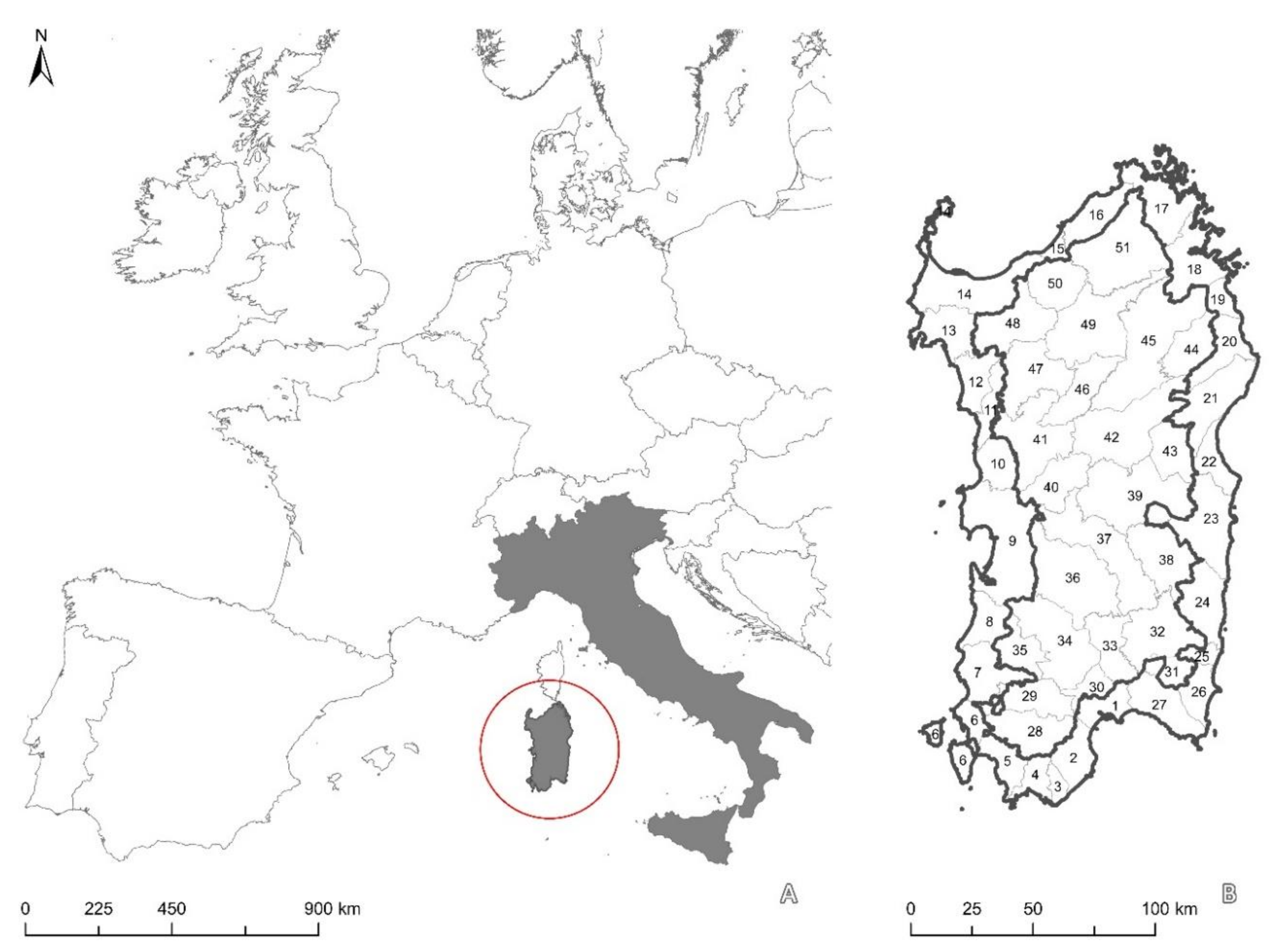
In this section, we illustrate the application of the CILF design method, starting (see step 1 in Table 1) from the choice of the decision-making units (DMU), i.e., the pool of spatial elementary units to be investigated and ranked according to their LF performance. In this respect, we refer to a decisional environment, where stakeholders are interested in analysing and managing LF throughout the region of Sardinia, Italy (Figure 1A). Sardinia is the second largest Italian island with a surface area of about 24,000 square kilometres. The island is scarcely populated though, as it hosts about 1.6 million inhabitants. Sardinia is an autonomous region with special authority on landscape management and planning. The main strategic/coordinator planning tool is the Regional Landscape Plan (RLP), which was approved in 2006 [16]. This plan attains landscape protection and enhancement and is designed according to the principles of the European Landscape Convention, the first supranational act ever able to factually influence planning practice over an entire continent [48]. The RLP is innovative, as it belongs to the last generation of landscape planning tools approved by more than a half of the Italian regional administrations [49]. So far, the RLP is active on the first homogeneous part including nearly 200 coastal municipalities and organized in 27 landscape units (LUs). As for the remaining and interior part of the island, planning unofficial documents, i.e., preparatory studies toward a new release and extended version of the RLP, refer to other 24 LUs. LUs represent the core part of the RLP: the corresponding documents (i.e., catalogues and atlas) offer a synthesis of the spatial knowledge on environmental, historical, and settlement systems and the general dispositions on the main measures to be developed on Sardinian landscapes. Given this key role, we select the LUs as DMUs of our investigations: the spatial pattern of the LUs is illustrated in Figure 1B.
We obtained the values of the three indicators for the 51 LUs and for two years (2003 and 2008) by processing spatial information, whose metadata is reported in Table 2. We stress that these datasets are the most updated information concerning land use and officially disseminated by the Autonomous Region of Sardinia.
Information concerning the geography of Sardinia and, typically, polygonal elements was obtained by processing the Land Use map available for free at the institutional website of the regional administration. Sardinia Geoportal is the interface of the regional geographic information system and the related spatial data infrastructure. The three indicators have been calculated by applying advanced geographical analysis and processing spatial data sets in shapefile in the GIS environment provided by QGIS (https://www.qgis.org/it/site/) and standard spreadsheet programs (Microsoft Excel). In Table 3, we report the values of the indicators. In the last rows of Table 3, we include the mean values of the indicators including all, then segmenting out only coastal and only internal LUs. Some phenomena can be analysed immediately, by scrutinizing the values of the three LF metrics. The first evidence is that, on average, LF of coastal LUs is much higher than on internal LUs. This is explained by the historically more intense development of coastal areas in Sardinia, like many other regions worldwide. In addition, this difference confirms that the indicators are reliable, i.e., they correctly picture the spatial pattern of the actual interplay between settlements and landscape in Sardinia.
As for the coastal part, for both the years, some LUs display high IFI, UFI and Seff values (Golfo di Oristano and Golfo dell’Asinara), some others low figures (Chia and Salto di Quirra). As for the internal areas, for both the years, a high LF is reported in some LUs (Regione delle giare basaltiche and Altopiani di Macomer), while a low LF is described in some other LUs (Serpeddì-Monte Genis and Supramonti interni). Still, some criticalities prevent analysts and decision-makers from elaborating an easy interpretation of the preliminary results. The data set reported in Table 3 is inhomogeneous, as figures present a variety of expressions and distributions. In this situation, the use of the three indicators for decision-making may lead to difficult interpretation. Hence, there is a desire to simplify the decisional process by adopting the CILF, a unique measure obtained as a combination of the three indicators of LF and able to capture the concepts conveyed by the three metrics into just one index.
We are now confronted with the choice of the most efficient way to obtain our CILF (see steps 3, 4, and 5 in Table 1). There are many alternatives available, as different expressions of our CI derive from the various possible indicators’ normalization and aggregation procedures presented in Section 3. For ease of presentation, we focus in this paper on the CILF release obtained by: (i) normalizing the indicators, according to the min-max algorithm, (ii) attaching the same relative importance (i.e., weight) to the indicators, and (iii) aggregating the indicators, according to the generalized geometric mean with parameter β equal to 0.50. We choose this triad, since the min-max algorithm leads to values ranging from 0 to 1 and is immediately comprehensible also by non-expert decision-makers and the generalized geometric mean offers an excellent aggregation method, which mixes in a balanced way compensatory and non-compensatory functions.
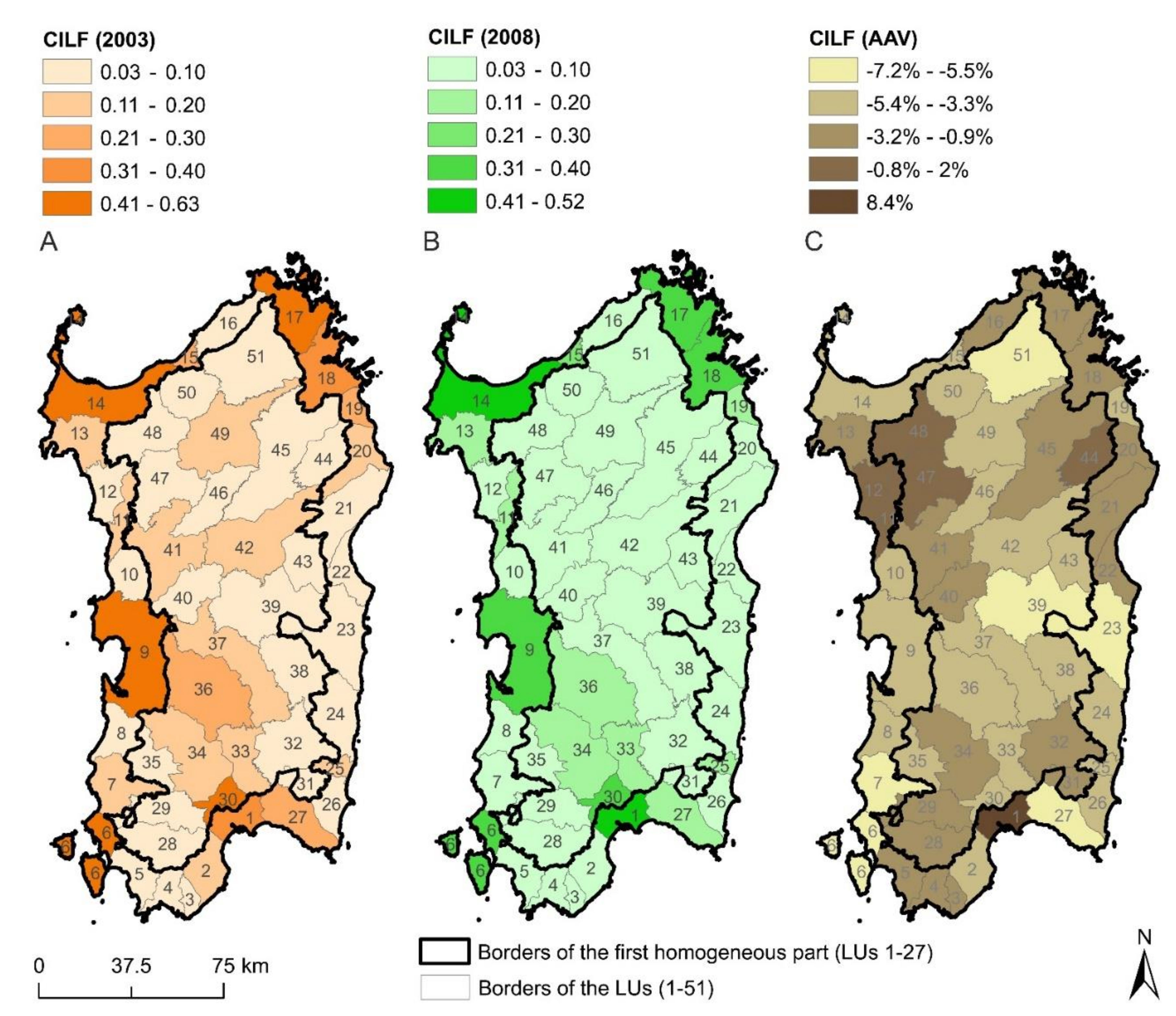
In Table 4, we report the values of the indicators normalized through the min-max transformation for the years 2003 and 2008 and the figures of the CILF version obtained after grouping the indicators’ values according to the GGM agglomeration rule described in Equation (7). The last column in Table 4 reports the average annual variation (AAV) of CILF in the time period considered. The value of the correlation coefficient (equal to 0.04) between the AAV of CILF and the initial value of CILF is a clear sign that, without management and planning, LF evolves randomly. In Figure 2, we map the values of CILF in 2003 and 2008 and the AAV.
The analyses of Figure 2 confirm that CILF is higher for LUs included in the coastal part of the RLP in both the years considered with a leading role played by LUs located in the metropolitan area of Cagliari, the capital town (n. 1 and 30), in the south western islands (n. 6), in the Oristano subregion (n. 9), in the Sassari-Alghero conurbation (n. 14 and 15), and in the so-called Emerald Coast the well-known touristic area in the North-East of the island (n. 17, 18, and 19). In addition, CILF is higher for the LUs (n. 1, 9, 30, and 36) belonging to the Campidano, a major plain for agricultural production and mobility infrastructures. As for the AAV of CILF, the most dynamic LUs are in the Cagliari area (n. 1) and in the Logudoro zone (n. 11, 12, 47, and 48). In addition, LUs of the Emerald Coast (n. 16, 17, and 18) and other coastal areas (n. 3, 4, 5, 20, 21, and 22) show higher AAV CILF figures with respect to the other LUs.
The interpretation of the results obtained is easy and supports decision-making efficiently, provided that the CI chosen in our example is proved reliable, i.e., so robust that other CIs obtained using other indicator normalization and aggregation rules supply similar outcomes. We ascertain the robustness by studying the sensitivity of CILF to the variations of normalization and aggregation modes. In Table 5 and Table 6, we report the values of ASR (see equation 11) calculated for the year 2003 and, respectively, 2008. The values of ASR (typically, those involving CILFMMGGM marked in bold Italic) are always lower than 1 position and signal a high robustness of CILF, with respect to all the selected alternative ways of obtaining CILF. This implies that had we chosen another CILF expression, the resulting ranking of DMUs, and the characteristics of the suggestions for decision-makers, would have been, on average, very similar.
However, a finer inspection of the shifts in ranking warns us from a simplistic selection of the correct CILF. In Table 7, we report on the mean, maximum, and minimum values of ASR, maximum shift in ranking (SRmax), minimum shift in ranking (SRMin), share of lower than 5 shifts in ranking (SSRunder 5), and share of lower than 10 shifts in ranking (SSRunder 10). While the statistics for ASR suggest a good robustness, the entire pool of pairwise evaluations of CILF rankings signals that SRmax oscillates in a remarkable range around a mean of 12 positions earned in 2003 and, likewise, SRmin ranges in an even larger interval up to 37 position lost in 2008. The picture is completed by the fair values of SSR referred to the number of times ranks vary by less than 5 or 10 positions (around 50% and 60% for both years).
The interplay between general robustness and local volatility reminds us that solutions that hold on average often do not, when dealing with individual cases. In this respect, we repeat the same analyses of Table 7 for the smaller pool of pairwise ranking comparisons involving only CILFMMGGM. Results are reported in Table 8: emerging evidence shows that SRMin, i.e., the minimum number of positions lost, decreases by 20 points, while maximum values of both SSRunder 5 and SSRunder 10 drop by 20 percentage points. In front of the promising, but still controversial, suggestions of Table 8, the selection of the eventual release of CILF should be supported also by the scrutiny of the detailed impact on the position in rank occupied by each DMU. In this respect, we report, in Table A1 (in Appendix A), the ranking shift each LU would receive, if we chose a different CILF release instead of CILFMMGGM. In the panorama of the four exemplary alternative expressions selected in Table A1, two main results emerge. First, the majority of LUs positions does not change much (i.e., by more than 3 positions). Secondly, the greatest variations in ranking (i.e., equal and larger than 10 positions) affect a few LUs in both the years considered. Before the eventual selection of the CILF expression, a finer investigation on the reasons of this variability (attaining LUs n. 3, 12, 25, and 31) is required and possible mitigation measures should be worked out.
Summarizing the main outcomes of this study, we have used an ensemble of three measures and a unique composite indicator to gauge spatial patterns and dynamics of LF throughout the landscape units of Sardinia. The indication of the simple indicators is confirmed by the values of the CILF, since LF is registered with higher intensity in coastal areas in both the years 2003 and 2008. This is relevant, as the composite indicator offers reliable indications on real processes. In this perspective, we obtained that CILF variation from 2003 to 2008 does not show any relevant correlation with the initial value of CILF in 2003. The absence of evidence of convergence or divergence may be a sign of the lack of policies explicitly designed to address LF processes over the island. Secondly, the indications of the CILF should be read and interpreted in connection with the patterns of the three simple LF indicators considered in this exercise. CILF signs should be traced back and confronted with the evidence coming from the IFI, UFI, and Seff. In this way, a more complete picture emerges from the interplay between CILF and original indexes and reminds us that a final fideistic use of just one “magic” indicator can be interpreted as driven by the illusions of reductionism. A third relevant outcome stems from the sensitivity analysis focussing on the robustness of the algorithm adopted to operationalize the CILF. This is based on a combination of (i) min-max normalization of the original simple indicators and (ii) the aggregation rule implying the generalized geometric mean of the normalized indicators. Apart from the manifold analysis, the main result is that the CILF designed in this paper generally offers 51 landscape units ranking that is robust, i.e., very similar, to the alternative ranking connected to the use of a CILF differently designed. This encouraging result still warns us against neglecting singular local effects, i.e., very high shifts in ranking, that deserve further focus and ad hoc integration.
5. Discussion
In this section, we discuss the results of this paper, with a general perspective and a special focus for the research questions (RQs) described in the Introduction. As a general outcome, this paper presents promising evidence on the possibility of tackling complexity by adopting CIs representing in a unique expression the accomplishment of many tasks or conditions. This brings about a clear advantage and simplification for practitioners supporting decision-makers confronted with the selection of multi-fold courses of action. At the same time, our exercise shows that simplification itself, introduced using a given CI, implies certainly a loss of information. The reduction of the suggestions coming from three indicators to the narrower hints of just one CI can never be considered as a neutral operation. This holds even with a stronger emphasis for local administrations committed to public funding management. Some DMUs may be advantaged or not by the adoption of a ranking connected to certain CI versus another one. The argument is clarified, with reference to the RQs. As for RQ1 concerning the possibility to construct a CI able to picture LF evolution in space and time, we have demonstrated that, starting from the guidelines of the HCCI [15], it is possible to tailor a method to designing the CILFMMGGM. This CI encapsulates the meaning of three LF indicators, which are calculated for the 51 LUs of the RLP of Sardinia and in two years. Thus, our composite indicator serves the cause of providing analysts and decision-makers with a single unifying measure of the evolution of LF in space (all over the LUs of Sardinia) and time (from 2003 to 2008). As for RQ2 concerning the robustness of the CI adopted, we have applied a sensitivity analysis to show that the position in ranking of each DMU, on average, is not sensible to the patterns of indicator normalization and aggregation. This implies that had we selected another CI, say the CILFBAM, the resulting ranking would have not changed much. This does not hold for all the DMUs though. We complemented our analysis with a finer inspection of the SR and demonstrated that the position in ranking of a few LUs would be severely affected (i.e., by more than 10 points) by the selection of other CILF formulations (derived from different indicator normalization/aggregation combinations). It is another possible confirmation that the selection of a CI should be carefully discussed and introduced in the decisional context, in front of the possible consequences on the procedures supported. As for the third RQ3 attaining the use of the CILF in the analysis and planning of Sardinian landscapes, we have demonstrated how the CILF provides the analyst with useful indications for understanding and monitoring the evolution of LF in space and time. The interplay between AAV CILF and the initial value (CILF in 2003) suggests that from 2003 to 2008 LF has evolved throughout the island with a random pattern. This implies that it is not possible to ascertain a movement of LUs toward convergence (higher LF LUs grow less than lower LF ones) or divergence (otherwise). This is important evidence for decision-makers interested in managing policies addressed to obtaining the achievement of a certain LF spatial pattern. For instance, certain policymakers could be concerned with maintaining a certain LF divide between coastal and internal LUs. Other policymakers may be inspired by a more balanced interplay between conservation and development and look forward to the increase of LF, provided that the required settlements and transport and mobility infrastructures are realized.
6. Conclusions
In this section, we present the concluding messages of this paper. We have developed on the CILF, a CI able to picture LF considering in a unique expression many concerns embedded in the three original LF indicators involved. The use of the CILF is intended for analytical and decision-making purposes, as it allows a simplification in the interpretation of a unique metric. This simplification in the decisional arenas can be admitted, provided that the rationale of the CILF design is made clear for all practitioners involved. In this respect, this paper provides the reader with a plain, and relatively easy to communicate, method for addressing the construction of the composite indicator at hand. The method is grounded in the HCCI [15], an authoritative, well-known and often adopted text. Ideally, the fundamental steps of the methods should be explained and clarified to stakeholders and decision-makers, in order to use the CILF in the most efficient and conscious way.
We feel that this study enriched the discourse in landscape planning in both practical and scientific terms. It provides a quite rare case study with a complete dataset, and offers promising evidence on the possibility of tackling complexity by adopting CIs that summarize three or more views of the same subject (i.e., LF) incorporated in one complex indicator at once. This leads to a system able to support policymakers, who are able to visualize results and maps via an intuitive graphic representation. However, we are aware of the information we loss when we use a CI. Thus, we question that CILF spatial patterns and dynamics should be interpreted in comparison with the corresponding trends of the simple indicators (i.e., IFI, UFI, and Seff). Furthermore, this study suggests that a wise reading of the CILF may support planners and policymakers in addressing the most efficacious measures for managing LF at the regional scale.
We have applied the method to the issue of LF monitoring and policymaking, but we advocate that it can be easily and successfully exported and applied to other decisional contexts showing diverse characteristics. In this respect, we would like to stress the scientific boundaries of our exercise and open future research paths. First, our CILF is provided as a combination of three indicators of LF, but it could be expanded to the many other LF metrics available in the literature. The extension can be performed with some caveats: the pool of indicators is complete and not redundant, i.e., they should represent all the concerns of the decision-makers without overlapping, and the indicators are independent, i.e., they are not correlated with each other. Secondly, we have developed an unweighted release of a CILF by assuming that all indicators have the same importance. We know that weighting is an Hamletian issue though. In decision-making, weighting serves the cause of a stronger awareness by practitioners on the agreement to attribute certain prevalence coefficients to each indicator. Weights can be extracted through multivariate (i.e., factor) analysis or processing the opinion of experts and stakeholders. There has not been space for developing these issues in this paper. We will work on developing a weighted release of a CILF in future studies.
Author Contributions
Conceptualization: A.D.M.; Methodology: A.D.M.; Formal Analysis: V.S. and A.G.; Investigation: A.D.M., V.S., A.G. and A.L.; Writing—Original Draft Preparation: A.D.M.; Writing—Review and Editing: A.D.M. and A.L.; Supervision: A.D.M.; Data Curation: V.S. All authors have read and agreed to the published version of the manuscript.
Funding
This work was funded by the Autonomous Region of Sardinia, research agreement “Paesaggi rurali della Sardegna—Riconoscimento delle componenti storiche, culturali ed insediative [Rural landscapes of Sardinia—Defining historical-cultural components and settlements]” and research project “Paesaggi rurali della Sardegna: pianificazione di infrastrutture verdi e blu e di reti territoriali complesse [Rural landscapes of Sardinia: planning green and blue infrastructures and complex spatial networks]”, Fondo per lo Sviluppo e la Coesione [Fund for the Development and Cohesion].
Acknowledgments
Andrea De Montis and Antonio Ledda are supported by the University of Sassari through the Fondo di Ateneo per la Ricerca [Academic funding for research activities] 2020.
Conflicts of Interest
The authors declare no conflict of interest.
Appendix A

Table A1.
Variability of the shift in ranking (SR) by LUs and years in four exemplary pairwise ranking comparisons. A few LUs (see marked in bold Italic) suffer from relevant (greater than 10 position acquired or lost) rank variations.
Table A1.
Variability of the shift in ranking (SR) by LUs and years in four exemplary pairwise ranking comparisons. A few LUs (see marked in bold Italic) suffer from relevant (greater than 10 position acquired or lost) rank variations.
| LU | 2003 | 2008 | ||||||
|---|---|---|---|---|---|---|---|---|
| CILFBAM Rank | CILFMMAM Rank | CILFMAM Rank | CILFBGM Rank | CILFBAM Rank | CILFMMAM Rank | CILFMAM Rank | CILFBGM Rank | |
| N | vs. CILFMMGGM rank | vs. CILFMMGGM rank | ||||||
| 1 | −4 | 0 | 0 | −2 | 2 | 0 | 0 | 0 |
| 2 | 2 | 0 | 0 | 1 | 1 | 1 | 1 | 2 |
| 3 | 13 | −11 | −10 | −4 | 12 | −11 | −11 | 1 |
| 4 | 1 | −3 | −3 | −4 | 0 | −9 | −8 | −7 |
| 5 | −5 | 4 | 4 | 0 | −4 | −1 | −1 | −3 |
| 6 | −3 | 0 | 0 | −2 | −3 | 0 | 0 | −1 |
| 7 | 3 | 2 | 2 | 7 | 1 | −1 | −1 | 5 |
| 8 | −3 | 0 | 0 | −1 | −1 | 3 | 3 | 2 |
| 9 | 3 | 1 | 1 | 2 | 2 | 1 | 1 | 3 |
| 10 | −3 | 0 | 0 | −2 | −4 | −1 | −1 | −2 |
| 11 | −5 | 2 | 3 | −5 | 0 | 1 | 1 | −1 |
| 12 | −12 | −1 | −1 | −14 | −7 | 1 | 1 | −7 |
| 13 | −3 | 2 | 1 | −1 | −3 | 3 | 2 | −1 |
| 14 | 1 | 0 | 0 | 0 | 2 | 0 | 0 | 0 |
| 15 | 3 | 0 | 0 | 0 | 3 | 0 | 0 | 0 |
| 16 | 1 | 2 | 1 | 4 | 3 | 3 | 3 | 7 |
| 17 | −1 | 0 | 0 | 1 | 1 | 0 | 0 | 2 |
| 18 | 0 | 0 | 0 | 1 | −4 | 0 | 0 | −3 |
| 19 | 1 | 1 | 1 | 0 | 1 | 0 | 0 | 0 |
| 20 | −5 | 2 | 2 | 6 | −6 | 3 | 3 | −2 |
| 21 | 1 | 4 | 4 | 4 | 0 | 4 | 4 | 1 |
| 22 | −3 | 0 | 0 | −4 | −5 | −2 | −2 | −6 |
| 23 | −2 | −5 | −5 | 1 | 0 | 2 | 1 | 2 |
| 24 | 7 | 2 | 2 | 8 | 3 | 1 | 1 | 3 |
| 25 | 8 | −3 | −3 | 1 | 11 | −3 | −2 | 5 |
| 26 | −1 | −5 | −5 | −1 | −1 | −4 | −3 | −2 |
| 27 | 2 | −1 | −1 | 0 | 2 | −1 | −1 | 3 |
| 28 | 7 | 1 | 1 | 8 | 6 | 2 | 2 | 6 |
| 29 | 2 | 0 | 0 | 5 | 3 | −3 | −3 | 6 |
| 30 | 4 | −1 | −1 | 0 | 3 | −1 | −1 | −1 |
| 31 | −3 | −9 | −8 | −14 | −2 | −12 | −12 | −12 |
| 32 | −3 | 0 | 0 | −3 | −1 | 3 | 3 | −1 |
| 33 | −4 | 2 | 2 | 0 | −4 | 4 | 4 | −1 |
| 34 | 0 | 2 | 2 | 0 | −1 | 1 | 1 | −1 |
| 35 | −7 | −1 | −1 | −3 | −5 | 0 | 1 | 1 |
| 36 | 6 | 0 | 0 | 1 | 7 | 0 | 0 | 1 |
| 37 | 3 | 4 | 4 | −4 | 4 | 0 | −1 | −3 |
| 38 | −1 | 4 | 4 | 0 | −2 | 1 | 1 | −1 |
| 39 | 1 | 0 | 0 | 1 | 1 | 1 | 1 | 1 |
| 40 | −5 | 6 | 6 | 1 | −4 | 3 | 3 | 1 |
| 41 | 9 | 2 | 1 | 0 | 5 | 0 | 0 | −1 |
| 42 | 4 | 0 | 0 | −2 | −3 | −2 | −2 | −7 |
| 43 | 1 | 0 | 0 | 0 | 0 | −2 | −2 | 0 |
| 44 | −3 | 1 | 1 | −2 | −6 | 2 | 2 | −4 |
| 45 | −1 | 0 | 0 | −2 | −1 | −1 | −1 | −1 |
| 46 | 5 | 3 | 3 | 6 | 4 | 5 | 5 | 5 |
| 47 | 1 | 5 | 5 | 4 | −2 | 3 | 3 | 3 |
| 48 | −2 | 3 | 3 | 1 | 1 | 5 | 5 | 3 |
| 49 | 2 | −3 | −3 | 1 | −5 | −1 | −2 | −2 |
| 50 | −1 | −5 | −5 | 3 | 5 | 0 | 0 | 5 |
| 51 | 0 | −7 | −7 | 3 | 2 | 2 | 2 | 3 |
References
- Blancas, F.J.; Lozano-Oyola, M.; González, M. A european sustainable tourism labels proposal using a composite indicator. Environ. Impact Assess. Rev. 2015, 54, 39–54. [Google Scholar] [CrossRef]
- Nardo, M.; Saisana, M. OECD/JRC Handbook on Constructing Composite Indicators. Putting Theory into Practice 2009. Available online: https://ec.europa.eu/eurostat/documents/1001617/4398416/S11P3-OECD-EC-HANDBOOK-NARDO-SAISANA.pdf (accessed on 17 November 2020).
- Karagiannis, R.; Karagiannis, G. Constructing composite indicators with Shannon entropy: The case of Human Development Index. Socio Econ. Plan. Sci. 2020, 70. [Google Scholar] [CrossRef]
- Attardi, R.; Cerreta, M.; Sannicandro, V.; Torre, C.M. Non-compensatory composite indicators for the evaluation of urban planning policy: The Land-Use Policy Efficiency Index (LUPEI). Eur. J. Oper. Res. 2018, 264, 491–507. [Google Scholar] [CrossRef]
- Zhang, L.P.; Zhou, P.; Qiu, Y.Q.; Su, Q.; Tang, Y.L. Reassessing the climate change cooperation performance via a non-compensatory composite indicator approach. J. Clean. Prod. 2020, 252, 119387. [Google Scholar] [CrossRef]
- European Environment Agency. Landscape Fragmentation in Europe, Joint EEA-FOEN Report; European Environment Agency: Copenhagen, Denmark, 2011; ISBN 978-92-9213-215-6. [Google Scholar]
- Jaeger, J.A.G. Landscape division, splitting index, and effective mesh size: New measures of landscape fragmentation. Landsc. Ecol. 2000, 15, 115–130. [Google Scholar] [CrossRef]
- Harris, L.D. The Fragmented Forest: Island Biogeography Theory and the Preservation of Biotic Diversity; University of Chicago Press: Chicago, IL, USA, 1984; ISBN 978-0-226-31764-9. [Google Scholar]
- Saunders, D.A.; Hobbs, R.J.; Margules, C.R. Biological consequences of ecosystem fragmentation: A review. Conserv. Biol. 1991, 5, 18–32. [Google Scholar] [CrossRef]
- Forman, R.T.T. Land Mosaics: The Ecology of Landscapes and Regions; Cambridge University Press: Cambridge, UK, 1995; ISBN 978-0-521-47462-7. [Google Scholar]
- United Nations. World Urbanization Prospects: The 2014 Revision, Highlights (ST/ESA/SER.A/352); Department of Economic and Social Affairs, Population Division: New York, NY, USA, 2014. [Google Scholar]
- Jaeger, J.A.G.; Bertiller, R.; Schwick, C.; Kienast, F. Suitability criteria for measures of urban sprawl. Ecol. Indic. 2010, 10, 397–406. [Google Scholar] [CrossRef]
- Romano, B. Evaluation of urban fragmentation in the ecosystems. In Proceedings of the International Conference on Mountain Environment and Development (ICMED), Chengdu, China, 20–26 May 2002. [Google Scholar]
- Floridi, M.; Pagni, S.; Falorni, S.; Luzzati, T. An exercise in composite indicators construction: Assessing the sustainability of Italian regions. Ecol. Econ. 2011, 70, 1440–1447. [Google Scholar] [CrossRef]
- OECD. Handbook on Constructing Composite Indicators: Methodology and User Guide; Organisation for Economic Co-operation and Development: Paris, France, 2008; ISBN 978-92-64-04345-9. [Google Scholar]
- Autonomous Region of Sardinia. Decree of the President of the Region n. 82, 7 September 2006, Approval of the Regional Landscape Plan-First Homogeneous Part-Decision of the Regional Government n. 36/7, 5 September 2006, Official Bulletin of the Autonomous Region of Sardinia, 58(30), 8 September 2006; Autonomous Region of Sardinia: Sardinia, Italy, 2006. [Google Scholar]
- Bunge, M. What is a quality of life indicator? Soc. Indic. Res. 1975, 2, 65–79. [Google Scholar] [CrossRef]
- Abberger, K.; Graff, M.; Siliverstovs, B.; Sturm, J.-E. Using rule-based updating procedures to improve the performance of composite indicators. Econ. Model. 2018, 68, 127–144. [Google Scholar] [CrossRef]
- Ciommi, M.; Gigliarano, C.; Emili, A.; Taralli, S.; Chelli, F.M. A new class of composite indicators for measuring well-being at the local level: An application to the Equitable and Sustainable Well-being (BES) of the Italian Provinces. Ecol. Indic. 2017, 76, 281–296. [Google Scholar] [CrossRef]
- Gómez-Vega, M.; Picazo-Tadeo, A.J. Ranking world tourist destinations with a composite indicator of competitiveness: To weigh or not to weigh? Tour. Manag. 2019, 72, 281–291. [Google Scholar] [CrossRef]
- Rogge, N. On aggregating Benefit of the Doubt composite indicators. Eur. J. Oper. Res. 2018, 264, 364–369. [Google Scholar] [CrossRef]
- Mendola, D.; Volo, S. Building composite indicators in tourism studies: Measurements and applications in tourism destination competitiveness. Tour. Manag. 2017, 59, 541–553. [Google Scholar] [CrossRef]
- Omrani, H.; Valipour, M.; Jafari Mamakani, S. Construct a composite indicator based on integrating Common Weight Data Envelopment Analysis and principal component analysis models: An application for finding development degree of provinces in Iran. Socio-Econ. Plan. Sci. 2019, 68, 100618. [Google Scholar] [CrossRef]
- Badea, A.C.; Rocco, S.C.M.; Tarantola, S.; Bolado, R. Composite indicators for security of energy supply using ordered weighted averaging. Reliab. Eng. Syst. Saf. 2011, 96, 651–662. [Google Scholar] [CrossRef]
- Miller, P.; De Barros, A.G.; Kattan, L.; Wirasinghe, S.C. Managing uncertainty in the application of composite sustainability indicators to transit analysis. Transp. Res. Procedia 2017, 25, 4003–4018. [Google Scholar] [CrossRef]
- Requejo-Castro, D.; Giné-Garriga, R.; Pérez-Foguet, A. Bayesian network modelling of hierarchical composite indicators. Sci. Total Environ. 2019, 668, 936–946. [Google Scholar] [CrossRef]
- Zanella, A.; Camanho, A.S.; Dias, T.G. Undesirable outputs and weighting schemes in composite indicators based on data envelopment analysis. Eur. J. Oper. Res. 2015, 245, 517–530. [Google Scholar] [CrossRef]
- Caschili, S.; De Montis, A.; Trogu, D. Accessibility and rurality indicators for regional development. Comput. Environ. Urban Syst. 2015, 49, 98–114. [Google Scholar] [CrossRef]
- Ghosh, B.; Chakma, N. Composite indicator of land, water and energy for measuring agricultural sustainability at micro level, Barddhaman District, West Bengal, India. Ecol. Indic. 2019, 102, 21–32. [Google Scholar] [CrossRef]
- Xavier, A.; Costa Freitas, M.D.B.; Fragoso, R.; Rosário, M.D.S. A regional composite indicator for analysing agricultural sustainability in Portugal: A goal programming approach. Ecol. Indic. 2018, 89, 84–100. [Google Scholar] [CrossRef]
- Wang, H. A generalized MCDA-DEA (multi-criterion decision analysis-data envelopment analysis) approach to construct slacks-based composite indicator. Energy 2015, 80, 114–122. [Google Scholar] [CrossRef]
- Singh, R.K.; Murty, H.R.; Gupta, S.K.; Dikshit, A.K. An overview of sustainability assessment methodologies. Ecol. Indic. 2012, 15, 281–299. [Google Scholar] [CrossRef]
- Abenayake, C.C.; Mikami, Y.; Matsuda, Y.; Jayasinghe, A. Ecosystem services-based composite indicator for assessing community resilience to floods. Environ. Dev. 2018, 27, 34–46. [Google Scholar] [CrossRef]
- Alam, M.; Dupras, J.; Messier, C. A framework towards a composite indicator for urban ecosystem services. Ecol. Indic. 2016, 60, 38–44. [Google Scholar] [CrossRef]
- Mao, F.; Zhao, X.; Ma, P.; Chi, S.; Richards, K.; Clark, J.; Hannah, D.M.; Krause, S. Developing composite indicators for ecological water quality assessment based on network interactions and expert judgment. Environ. Model. Softw. 2019, 115, 51–62. [Google Scholar] [CrossRef]
- Speak, A.; Escobedo, F.J.; Russo, A.; Zerbe, S. An ecosystem service-disservice ratio: Using composite indicators to assess the net benefits of urban trees. Ecol. Indic. 2018, 95, 544–553. [Google Scholar] [CrossRef]
- Llauss, A.; Nogué, J. Indicators of landscape fragmentation: The case for combining ecological indices and the perceptive approach. Ecol. Indic. 2012, 15, 85–91. [Google Scholar] [CrossRef]
- Opdam, P.; Verboom, J.; Pouwels, R. Landscape cohesion: An index for the conservation potential of landscapes for biodiversity. Landsc. Ecol. 2003, 18, 113–126. [Google Scholar] [CrossRef]
- Becker, W.; Saisana, M.; Paruolo, P.; Vandecasteele, I. Weights and importance in composite indicators: Closing the gap. Ecol. Indic. 2017, 80, 12–22. [Google Scholar] [CrossRef] [PubMed]
- Ruiz, F.; El Gibari, S.; Cabello, J.M.; Gómez, T. MRP-WSCI: Multiple reference point based weak and strong composite indicators. Omega 2020, 95. [Google Scholar] [CrossRef]
- Luzzati, T.; Gucciardi, G. A non-simplistic approach to composite indicators and rankings: An illustration by comparing the sustainability of the EU Countries. Ecol. Econ. 2015, 113, 25–38. [Google Scholar] [CrossRef]
- Bruschi, D.; Astiaso Garcia, D.; Gugliermetti, F.; Cumo, F. Characterizing the fragmentation level of Italian’s National Parks due to transportation infrastructures. Transp. Res. Part D Transp. Environ. 2015, 36, 18–28. [Google Scholar] [CrossRef]
- Astiaso Garcia, D.; Bruschi, D.; Cinquepalmi, F.; Cumo, F. An estimation of urban fragmentation of natural habitats: Case studies of the 24 italian national parks. Chem. Eng. Trans. 2013, 32, 49–54. [Google Scholar] [CrossRef]
- Battisti, C.; Romano, B. Frammentazione e Connettività. Dall’analisi Ecologica alla Pianificazione Ambientale; Città Studi: Torino, Italy, 2007; ISBN 978-88-251-7314-7. [Google Scholar]
- Biondi, M.; Corridore, G.; Romano, B.; Tamburini, G.; Tetè, P. Evaluation and planning control of the ecosystem fragmentation due to urban development. In Proceedings of the 50th Conference of the European Regional Science Association (ERSA), Jyväskylä, Finland, 27–30 August 2003. [Google Scholar]
- Romano, B.; Zullo, F. Valutazione della pressione insediativa: Indicatori e sperimentazione di soglie. In Biodiversità, Disturbi, Minacce; Battisti, C., Conigliaro, M., Poeta, G., Teofili, C., Eds.; Editrice Universitaria Udinese: Udine, Italy, 2013; pp. 170–177. ISBN 978-88-8420-803-3. [Google Scholar]
- Battisti, C.; Conigliaro, M.; Poeta, G.; Teofili, C. Biodiversità, Disturbi, Minacce. Dall’ecologia di Base alla Gestione e Conservazione Degli Ecosistemi; Forum Edizioni: Udine, Italy, 2013; ISBN 978-88-8420-803-3. [Google Scholar]
- De Montis, A. Impacts of the European Landscape Convention on national planning systems: A comparative investigation of six case studies. Landsc. Urban Plan. 2014, 124, 53–65. [Google Scholar] [CrossRef]
- De Montis, A. Measuring the performance of planning: The conformance of Italian landscape planning practices with the European Landscape Convention. Eur. Plan. Stud. 2016, 24, 1727–1745. [Google Scholar] [CrossRef]
Figure 1.
(A). The red circle identifies the location of Sardinia (Italy), in the context of the western Mediterranean basin. (B). The Decision-Making Units consist of the 51 Landscape Units of the Regional Landscape Plan (RLP) of Sardinia. The thick line divides coastal from interior landscape units (LUs).

Figure 2.
Spatial analysis of CILF in 2003 (A) and 2008 (B) and average annual variation (AAV) of CILF (C) throughout the 51 LUs of the RLP of Sardinia.
Figure 2.
Spatial analysis of CILF in 2003 (A) and 2008 (B) and average annual variation (AAV) of CILF (C) throughout the 51 LUs of the RLP of Sardinia.

Table 1.
The methodology adopted for building the composite indicator of landscape fragmentation (CILF): steps and rationale (after OECD [15] and Nardo and Saisana [2]).
| N | Description | Rationale |
|---|---|---|
| 1 | Theoretical framework | Simplification of decisional processes through the construction of a unique CILF for LF and considering three relevant aspects. The context is strategic landscape analysis and planning in a Mediterranean region: the DMUs correspond to the 51 landscape units designed by the Regional Landscape Plan of Sardinia [16]. |
| 2 | Variables | CILF derives from a combination of three indicators, IFI, UFI, and Seff, measuring LF due to transport and mobility infrastructure, urban settlements, and landscape subdivision per se in several patches. |
| 3 | Normalization | The indicators are normalized according to three transformations: distance of Borda, distance from minimum normalized by the range (min-max transformation), rescaling with respect to the maximum value. |
| 4 | Aggregation | Normalized indicators are aggregated by means of three rules: arithmetic, geometric, and generalized geometric mean. |
| 5 | Robustness and sensitivity | Sensitivity analysis is performed to ascertain the robustness of CILF expressions obtained according to the various normalization and aggregation patterns. Various metrics characterize the variation of the shift in ranking of the DMUs. |
Table 2.
Spatial data set used for calculating the indicators of landscape fragmentation.
| Key Elements | Data | Year | Scale | Source | Website |
|---|---|---|---|---|---|
| Patches, human settlements | Land Use map of Sardinia, areas | 2003, 2008 | 1:25,000 | Sardinia Geoportal, Autonomous Region of Sardinia | http://www.sardegnageoportale.it/ |
| Linear infrastructures | Land Use map of Sardinia, linear elements |
Table 3.
LF indicators values by year and landscape units. Mean values suggest that LF is much higher, on average, in coastal LUs. Seff values have been multiplied by 1000 and express the number of patches included in a surface area extending by 1000 km2 [6].
Table 3.
LF indicators values by year and landscape units. Mean values suggest that LF is much higher, on average, in coastal LUs. Seff values have been multiplied by 1000 and express the number of patches included in a surface area extending by 1000 km2 [6].
| RLP Landscape Units | Indicators (2003) | Indicators (2008) | ||||||
|---|---|---|---|---|---|---|---|---|
| Homogeneous Part | N | Denomination | IFI | UFI | Seff | IFI | UFI | Seff |
| Coastal | 1 | Golfo di Cagliari | 928.41 | 0.73 | 17.75 | 1265.16 | 3.62 | 18.49 |
| 2 | Nora | 135.19 | 0.57 | 3.54 | 134.35 | 0.89 | 3.68 | |
| 3 | Chia | 16.17 | 0.07 | 11.56 | 15.87 | 0.13 | 11.68 | |
| 4 | Golfo di Teulada | 91.88 | 0.02 | 5.19 | 92.06 | 0.04 | 5.20 | |
| 5 | Anfiteatro del Sulcis | 274.32 | 0.26 | 4.15 | 274.47 | 0.56 | 4.25 | |
| 6 | Carbonia e Isole sulcitane | 1855.18 | 1.59 | 11.46 | 1900.10 | 1.86 | 11.91 | |
| 7 | Bacino metallifero | 460.89 | 0.60 | 2.46 | 476.51 | 0.77 | 2.47 | |
| 8 | Arburese | 230.97 | 0.15 | 3.65 | 251.15 | 0.17 | 3.65 | |
| 9 | Golfo di Oristano | 13,959.40 | 1.35 | 2.57 | 14,267.11 | 1.71 | 3.17 | |
| 10 | Montiferru | 337.44 | 0.12 | 4.03 | 340.94 | 0.17 | 4.05 | |
| 11 | Planargia | 1122.35 | 0.13 | 5.22 | 1209.16 | 0.22 | 7.94 | |
| 12 | Monteleone | 747.12 | 0.01 | 3.41 | 780.40 | 0.04 | 3.42 | |
| 13 | Alghero | 2243.81 | 0.48 | 3.04 | 2225.22 | 0.96 | 3.13 | |
| 14 | Golfo dell’Asinara | 19,156.42 | 1.60 | 3.28 | 20,719.70 | 2.23 | 3.37 | |
| 15 | Bassa valle del Coghinas | 147.00 | 0.62 | 15.51 | 163.33 | 0.80 | 15.91 | |
| 16 | Gallura costiera nord-occidentale | 196.40 | 0.19 | 2.52 | 196.40 | 0.30 | 2.62 | |
| 17 | Gallura costiera nord-orientale | 13,290.97 | 0.99 | 3.05 | 13,797.54 | 1.65 | 3.07 | |
| 18 | Golfo di Olbia | 6028.91 | 1.44 | 2.42 | 6225.49 | 1.95 | 4.13 | |
| 19 | Budoni - S.Teodoro | 229.60 | 0.92 | 8.56 | 263.07 | 1.14 | 9.81 | |
| 20 | Monte Albo | 638.49 | 0.39 | 3.21 | 841.50 | 0.58 | 3.25 | |
| 21 | Baronia | 1297.30 | 0.19 | 1.76 | 1298.95 | 0.32 | 1.85 | |
| 22 | Supramonte di Baunei e Dorgali | 164.90 | 0.02 | 4.00 | 281.12 | 0.03 | 4.00 | |
| 23 | Ogliastra | 638.60 | 0.43 | 1.51 | 656.63 | 0.49 | 1.52 | |
| 24 | Salto di Quirra | 56.64 | 0.15 | 2.19 | 117.31 | 0.19 | 2.20 | |
| 25 | Bassa valle del Flumendosa | 107.67 | 0.23 | 10.07 | 117.49 | 0.27 | 10.15 | |
| 26 | Castiadas | 84.09 | 0.29 | 4.39 | 91.37 | 0.35 | 4.41 | |
| 27 | Golfo orientale di Cagliari | 755.98 | 1.41 | 2.52 | 783.48 | 1.57 | 2.52 | |
| Internal | 28 | Sulcis | 54.08 | 0.19 | 2.14 | 84.59 | 0.32 | 2.17 |
| 29 | Valle del Cixerri | 114.07 | 0.23 | 2.54 | 120.35 | 0.46 | 2.57 | |
| 30 | Basso Campidano | 218.89 | 1.33 | 23.19 | 396.05 | 1.66 | 24.60 | |
| 31 | Serpeddì-Monte Genis | 23.32 | 0.01 | 5.25 | 23.32 | 0.02 | 5.26 | |
| 32 | Gerrei | 453.67 | 0.05 | 1.68 | 568.60 | 0.07 | 1.68 | |
| 33 | Parteolla Trexenta | 2162.33 | 0.47 | 3.06 | 2352.74 | 0.71 | 3.13 | |
| 34 | Campidano | 2386.31 | 0.54 | 1.59 | 2423.93 | 1.02 | 1.64 | |
| 35 | Monte Linas | 427.44 | 0.18 | 4.00 | 433.93 | 0.27 | 4.01 | |
| 36 | Regione delle giare basaltiche | 9260.50 | 0.39 | 1.46 | 9522.59 | 0.49 | 1.47 | |
| 37 | Flumendosa-Sarcidano-Araxisi | 2844.21 | 0.23 | 1.31 | 3048.57 | 0.29 | 1.31 | |
| 38 | Regione dei tacchi calcarei | 507.99 | 0.06 | 1.87 | 508.89 | 0.06 | 1.86 | |
| 39 | Gennargentu e Mandrolisai | 250.39 | 0.10 | 1.02 | 251.51 | 0.11 | 1.02 | |
| 40 | Media valle del Tirso | 1406.12 | 0.18 | 2.66 | 1517.20 | 0.33 | 2.70 | |
| 41 | Altopiani di Macomer | 3770.56 | 0.17 | 1.55 | 3808.67 | 0.27 | 1.55 | |
| 42 | Valli del Rio Isalle e Liscoi | 2721.64 | 0.39 | 1.21 | 2677.18 | 0.49 | 1.21 | |
| 43 | Supramonti interni | 57.76 | 0.05 | 2.94 | 76.31 | 0.05 | 2.94 | |
| 44 | La valle del Rio Mannu | 332.31 | 0.03 | 2.90 | 567.71 | 0.05 | 2.91 | |
| 45 | Altopiani e Alta Valle del Tirso | 380.55 | 0.06 | 0.90 | 447.21 | 0.10 | 0.90 | |
| 46 | Marghine - Goceano | 115.84 | 0.15 | 2.61 | 303.31 | 0.16 | 2.62 | |
| 47 | Meilogu | 1347.16 | 0.17 | 1.80 | 1622.18 | 0.35 | 1.82 | |
| 48 | Logudoro | 1662.05 | 0.22 | 1.91 | 2049.52 | 0.47 | 1.95 | |
| 49 | Piana del Rio Mannu di Ozieri | 1393.85 | 0.38 | 1.21 | 1424.82 | 0.51 | 1.22 | |
| 50 | Anglona | 66.68 | 0.24 | 2.68 | 73.19 | 0.36 | 2.70 | |
| 51 | Massiccio del Limbara | 364.86 | 0.42 | 1.14 | 366.39 | 0.47 | 1.14 | |
| Mean values | All LUs | 1912.13 | 0.42 | 4.23 | 2028.52 | 0.63 | 4.44 | |
| Coastal LUs | 2414.67 | 0.55 | 5.30 | 2547.62 | 0.85 | 5.62 | ||
| Internal LUs | 1346.77 | 0.26 | 3.02 | 1444.53 | 0.38 | 3.10 | ||
Table 4.
CILF unweighted release obtained according to min-max (MM) normalization of the indicators and generalized geometric mean (GGM) aggregation rule.
Table 4.
CILF unweighted release obtained according to min-max (MM) normalization of the indicators and generalized geometric mean (GGM) aggregation rule.
| LU | MM-Normalized Indicators (2003) | MM-Normalized Indicators (2008) | GGM Aggregated CI | ||||||
|---|---|---|---|---|---|---|---|---|---|
| N | IFI | UFI | Seff | IFI | UFI | Seff | CILF (2003) | CILF (2008) | CILF (AAV) |
| 1 | 0.05 | 0.46 | 0.77 | 0.06 | 1.00 | 0.75 | 0.35 | 0.50 | 8.42% |
| 2 | 0.01 | 0.35 | 0.15 | 0.01 | 0.25 | 0.15 | 0.13 | 0.10 | −3.75% |
| 3 | 0.00 | 0.05 | 0.50 | 0.00 | 0.04 | 0.48 | 0.10 | 0.09 | −1.70% |
| 4 | 0.00 | 0.01 | 0.22 | 0.00 | 0.01 | 0.21 | 0.05 | 0.04 | −1.51% |
| 5 | 0.01 | 0.16 | 0.18 | 0.01 | 0.16 | 0.17 | 0.10 | 0.10 | −0.88% |
| 6 | 0.10 | 1.00 | 0.49 | 0.09 | 0.51 | 0.48 | 0.45 | 0.33 | −5.49% |
| 7 | 0.02 | 0.37 | 0.11 | 0.02 | 0.21 | 0.10 | 0.13 | 0.10 | −5.54% |
| 8 | 0.01 | 0.10 | 0.16 | 0.01 | 0.05 | 0.15 | 0.07 | 0.06 | −4.91% |
| 9 | 0.73 | 0.85 | 0.11 | 0.69 | 0.47 | 0.13 | 0.49 | 0.39 | −4.18% |
| 10 | 0.02 | 0.08 | 0.17 | 0.02 | 0.05 | 0.16 | 0.08 | 0.06 | −3.28% |
| 11 | 0.06 | 0.08 | 0.23 | 0.06 | 0.06 | 0.32 | 0.11 | 0.12 | 1.99% |
| 12 | 0.04 | 0.00 | 0.15 | 0.04 | 0.01 | 0.14 | 0.05 | 0.05 | 1.39% |
| 13 | 0.12 | 0.30 | 0.13 | 0.11 | 0.27 | 0.13 | 0.17 | 0.16 | −1.70% |
| 14 | 1.00 | 1.00 | 0.14 | 1.00 | 0.62 | 0.14 | 0.63 | 0.52 | −3.55% |
| 15 | 0.01 | 0.39 | 0.67 | 0.01 | 0.22 | 0.65 | 0.26 | 0.21 | −4.08% |
| 16 | 0.01 | 0.12 | 0.11 | 0.01 | 0.08 | 0.11 | 0.07 | 0.06 | −3.00% |
| 17 | 0.69 | 0.62 | 0.13 | 0.67 | 0.45 | 0.12 | 0.44 | 0.38 | −2.73% |
| 18 | 0.31 | 0.90 | 0.10 | 0.30 | 0.54 | 0.17 | 0.37 | 0.32 | −2.99% |
| 19 | 0.01 | 0.58 | 0.37 | 0.01 | 0.32 | 0.40 | 0.24 | 0.19 | −4.34% |
| 20 | 0.03 | 0.24 | 0.14 | 0.04 | 0.16 | 0.13 | 0.12 | 0.10 | −3.07% |
| 21 | 0.07 | 0.12 | 0.08 | 0.06 | 0.09 | 0.08 | 0.09 | 0.07 | −2.61% |
| 22 | 0.01 | 0.02 | 0.17 | 0.01 | 0.01 | 0.16 | 0.04 | 0.04 | −1.48% |
| 23 | 0.03 | 0.27 | 0.07 | 0.03 | 0.13 | 0.06 | 0.10 | 0.07 | −6.21% |
| 24 | 0.00 | 0.10 | 0.09 | 0.01 | 0.05 | 0.09 | 0.05 | 0.04 | −3.90% |
| 25 | 0.01 | 0.15 | 0.43 | 0.01 | 0.07 | 0.41 | 0.14 | 0.11 | −4.20% |
| 26 | 0.00 | 0.18 | 0.19 | 0.00 | 0.10 | 0.18 | 0.10 | 0.07 | −5.02% |
| 27 | 0.04 | 0.88 | 0.11 | 0.04 | 0.43 | 0.10 | 0.24 | 0.15 | −7.24% |
| 28 | 0.00 | 0.12 | 0.09 | 0.00 | 0.09 | 0.09 | 0.05 | 0.05 | −2.40% |
| 29 | 0.01 | 0.14 | 0.11 | 0.01 | 0.13 | 0.10 | 0.07 | 0.06 | −1.58% |
| 30 | 0.01 | 0.83 | 1.00 | 0.02 | 0.46 | 1.00 | 0.45 | 0.37 | −3.85% |
| 31 | 0.00 | 0.01 | 0.23 | 0.00 | 0.01 | 0.21 | 0.04 | 0.04 | −1.32% |
| 32 | 0.02 | 0.03 | 0.07 | 0.03 | 0.02 | 0.07 | 0.04 | 0.04 | −2.19% |
| 33 | 0.11 | 0.29 | 0.13 | 0.11 | 0.20 | 0.13 | 0.17 | 0.14 | −3.26% |
| 34 | 0.12 | 0.34 | 0.07 | 0.12 | 0.28 | 0.07 | 0.16 | 0.14 | −2.12% |
| 35 | 0.02 | 0.11 | 0.17 | 0.02 | 0.07 | 0.16 | 0.09 | 0.07 | −3.35% |
| 36 | 0.48 | 0.24 | 0.06 | 0.46 | 0.14 | 0.06 | 0.23 | 0.18 | −3.97% |
| 37 | 0.15 | 0.14 | 0.06 | 0.15 | 0.08 | 0.05 | 0.11 | 0.09 | −3.98% |
| 38 | 0.03 | 0.04 | 0.08 | 0.02 | 0.02 | 0.08 | 0.05 | 0.03 | −4.67% |
| 39 | 0.01 | 0.06 | 0.04 | 0.01 | 0.03 | 0.04 | 0.04 | 0.03 | −5.56% |
| 40 | 0.07 | 0.11 | 0.11 | 0.07 | 0.09 | 0.11 | 0.10 | 0.09 | −1.73% |
| 41 | 0.20 | 0.11 | 0.07 | 0.18 | 0.07 | 0.06 | 0.12 | 0.10 | −2.82% |
| 42 | 0.14 | 0.24 | 0.05 | 0.13 | 0.14 | 0.05 | 0.13 | 0.10 | −5.09% |
| 43 | 0.00 | 0.03 | 0.13 | 0.00 | 0.01 | 0.12 | 0.04 | 0.03 | −4.12% |
| 44 | 0.02 | 0.02 | 0.13 | 0.03 | 0.01 | 0.12 | 0.04 | 0.04 | 0.27% |
| 45 | 0.02 | 0.04 | 0.04 | 0.02 | 0.03 | 0.04 | 0.03 | 0.03 | −1.99% |
| 46 | 0.01 | 0.09 | 0.11 | 0.01 | 0.04 | 0.11 | 0.06 | 0.05 | −3.32% |
| 47 | 0.07 | 0.11 | 0.08 | 0.08 | 0.10 | 0.07 | 0.08 | 0.08 | −0.34% |
| 48 | 0.09 | 0.14 | 0.08 | 0.10 | 0.13 | 0.08 | 0.10 | 0.10 | 0.13% |
| 49 | 0.07 | 0.24 | 0.05 | 0.07 | 0.14 | 0.05 | 0.11 | 0.08 | −4.79% |
| 50 | 0.00 | 0.15 | 0.12 | 0.00 | 0.10 | 0.11 | 0.07 | 0.06 | −3.90% |
| 51 | 0.02 | 0.26 | 0.05 | 0.02 | 0.13 | 0.05 | 0.08 | 0.06 | −6.81% |
Table 5.
Sensitivity analysis of CILF calculated for 2003. Average shift in ranking values for couples of CILF metrics calculated according to different expressions. Indicators normalization rule codes: B for Borda distance, MM for min-max rescaling, and M for rescaling to the maximum. Normalized indicator aggregation rule codes: AM for arithmetic mean, GM for geometric mean, and GGM for generalized geometric mean. ASR values concerning pairwise comparisons of CILFMMGGM are marked in bold Italic.
| CILFBAM | CILFMMAM | CILFMAM | CILFBGM | CILFMMGM | CILFMGM | CILFBGGM | CILFMMGGM | CILFMGGM | |
|---|---|---|---|---|---|---|---|---|---|
| CILFBAM | 0.22 | 0.22 | 0.22 | 0.27 | 0.22 | 0.22 | 0.22 | 0.22 | |
| CILFMMAM | 0.00 | 0.00 | 0.06 | 0.00 | 0.00 | 0.00 | 0.00 | ||
| CILFMAM | 0.00 | 0.06 | 0.00 | 0.00 | 0.00 | 0.00 | |||
| CILFBGM | 0.06 | 0.00 | 0.00 | 0.00 | 0.00 | ||||
| CILFMMGM | −0.06 | −0.06 | −0.06 | −0.06 | |||||
| CILFMGM | 0.00 | 0.00 | 0.00 | ||||||
| CILFBGGM | 0.00 | 0.00 | |||||||
| CILFMMGGM | 0.00 | ||||||||
| CILFMGGM |
Table 6.
Sensitivity analysis of CILF calculated for 2008. Average shift in ranking values for couples of CILF metrics calculated according to different expressions. Indicators normalization rule codes: B for Borda distance, MM for min-max rescaling, and M for rescaling to the maximum. Normalized indicator aggregation rule codes: AM for arithmetic mean, GM for geometric mean, and GGM for generalized geometric mean. ASR values concerning pairwise comparisons of CILFMMGGM are marked in bold Italic.
| CILFBAM | CILFMMAM | CILFMAM | CILFBGM | CILFMMGM | CILFMGM | CILFBGGM | CILFMMGGM | CILFMGGM | |
|---|---|---|---|---|---|---|---|---|---|
| CILFBAM | 0.22 | 0.22 | 0.20 | 0.27 | 0.22 | 0.20 | 0.22 | 0.22 | |
| CILFMMAM | 0.00 | −0.02 | 0.06 | 0.00 | −0.02 | 0.00 | 0.00 | ||
| CILFMAM | −0.02 | 0.06 | 0.00 | −0.02 | 0.00 | 0.00 | |||
| CILFBGM | 0.08 | 0.02 | 0.00 | 0.02 | 0.02 | ||||
| CILFMMGM | −0.06 | −0.08 | −0.06 | −0.06 | |||||
| CILFMGM | −0.02 | 0.00 | 0.00 | ||||||
| CILFBGGM | 0.02 | 0.02 | |||||||
| CILFMMGGM | 0.00 | ||||||||
| CILFMGGM |
Table 7.
Analysis of the variation of the shift in ranking. The ASR values testify a very good robustness of CILF with respect to the variations of normalization and aggregation rules. The other measures describe a fair volatility of the shift in ranking.
Table 7.
Analysis of the variation of the shift in ranking. The ASR values testify a very good robustness of CILF with respect to the variations of normalization and aggregation rules. The other measures describe a fair volatility of the shift in ranking.
| 2003 | 2008 | |||||
|---|---|---|---|---|---|---|
| Mean | Max | Min | Mean | Max | Min | |
| ASR | 0.05 | 0.27 | 0.00 | 0.05 | 0.27 | 0.00 |
| SRmax | 12 | 25 | 1 | 11 | 26 | 1 |
| SRMin | −14 | −1 | −36 | −13 | −1 | −37 |
| SSRunder5 | 49.35% | 94.12% | 25.49% | 50.54% | 92.16% | 23.53% |
| SSRunder10 | 57.46% | 94.12% | 35.29% | 58.33% | 92.16% | 33.33% |
Table 8.
Analysis of the variation of the shift in ranking with a focus only on the pairwise comparisons involving the selected CILFMMGGM. The ASR values testify a very good robustness of CILF with respect to the variations of normalization and aggregation rules. The other measures describe a fair volatility of the shift in ranking.
| 2003 | 2008 | |||||
|---|---|---|---|---|---|---|
| Mean | Max | Min | Mean | Max | Min | |
| ASR | 0.02 | 0.22 | 0.00 | 0.03 | 0.22 | 0.00 |
| SRmax | 12 | 25 | 5 | 12 | 26 | 4 |
| SRMin | −10 | −5 | −14 | −9 | −3 | −12 |
| SSRunder5 | 54.90% | 72.55% | 31.37% | 51.82% | 68.63% | 29.41% |
| SSRunder10 | 59.66% | 74.51% | 39.22% | 54.90% | 68.63% | 37.25% |
Publisher’s Note: MDPI stays neutral with regard to jurisdictional claims in published maps and institutional affiliations. |
© 2020 by the authors. Licensee MDPI, Basel, Switzerland. This article is an open access article distributed under the terms and conditions of the Creative Commons Attribution (CC BY) license (http://creativecommons.org/licenses/by/4.0/).
Share and Cite
MDPI and ACS Style
De Montis, A.; Serra, V.; Ganciu, A.; Ledda, A. Assessing Landscape Fragmentation: A Composite Indicator. Sustainability 2020, 12, 9632. https://0-doi-org.brum.beds.ac.uk/10.3390/su12229632
AMA Style
De Montis A, Serra V, Ganciu A, Ledda A. Assessing Landscape Fragmentation: A Composite Indicator. Sustainability. 2020; 12(22):9632. https://0-doi-org.brum.beds.ac.uk/10.3390/su12229632
Chicago/Turabian StyleDe Montis, Andrea, Vittorio Serra, Amedeo Ganciu, and Antonio Ledda. 2020. "Assessing Landscape Fragmentation: A Composite Indicator" Sustainability 12, no. 22: 9632. https://0-doi-org.brum.beds.ac.uk/10.3390/su12229632
Note that from the first issue of 2016, this journal uses article numbers instead of page numbers. See further details here.