A Vector Map of Carbon Emission Based on Point-Line-Area Carbon Emission Classified Allocation Method

Abstract

An explicit spatial carbon emission map is of great significance for reducing carbon emissions through urban planning. Previous studies have proved that, at the city scale, the vector carbon emission maps can provide more accurate spatial carbon emission estimates than gridded maps. To draw a vector carbon emission map, the spatial allocation of greenhouse gas (GHG) inventory is crucial. However, the previous methods did not consider different carbon sources and their influencing factors. This study proposes a point-line-area (P-L-A) classified allocation method for drawing a vector carbon emission map. The method has been applied in Changxing, a representative small city in China. The results show that the carbon emission map can help identify the key carbon reduction regions. The emission map of Changxing shows that high-intensity areas are concentrated in four industrial towns (accounting for about 80%) and the central city. The results also reflect the different carbon emission intensity of detailed land-use types. By comparison with other research methods, the accuracy of this method was proved. The method establishes the relationship between the GHG inventory and the basic spatial objects to conduct a vector carbon emission map, which can better serve the government to formulate carbon reduction strategies and provide support for low-carbon planning.

1. Introduction

Urban planning plays an increasingly significant role in reducing carbon emissions, the most important factor for climate change mitigation. Many studies have illustrated that carbon emissions are highly influenced by land use and urban morphology [1,2,3]. Urban planning can help mitigate carbon emissions through the rational allocation of land use to improve energy efficiency and through optimization of the urban form to reduce traffic demand [4,5,6,7]. According to the research by Chuai et al. [8], about 12 percent reduction of energy-related carbon emissions can be obtained by adjustment of land use structure. Therefore, urban planning is a key technology in reducing carbon emissions.

The carbon emission map is an important basis for urban planning to reduce carbon emissions. Urban planning methods need information about where carbon emissions occur and how much is emitted within clear boundaries [9,10]. Since the carbon emission map can reflect the spatial distribution of carbon emissions, the emissions of different boundaries can be calculated from administrative units to land patches [11]. It allows researchers to compare the relative influences of each emission source and identify hot spots and unexpected emissions, which is useful for formulating targeted carbon reduction strategies and space optimization schemes [12,13,14]. By creating a land-use carbon emission map, Zhang et al. [9] analyzed the spatial distribution of city carbon emissions and found that most of the land used for carbon storage was located outside the city, while most land use types in the central region had high carbon emissions. On this basis, the low-carbon urban planning strategy was discussed from two aspects of structure and connection. Wang et al. [15] used the land-use carbon emission map to evaluate the impact of land use spatial attributes on carbon emissions by various landscape metrics. The results showed the distribution of carbon emissions per unit area of land use categories considering spatial attributes, which was very important for guiding the spatial organization of land use. Since carbon emission maps can be used as a quantitative and objective manner to support low-carbon planning, more and more studies have focused on the construction of carbon emission maps.

Most of the existing carbon emission maps are presented in the form of a spatial grid, also referred to as gridded emission maps. These gridded carbon emission maps are usually drawn by the grid allocation method of the greenhouse gas (GHG) inventory, which means decomposing the total carbon emissions of GHG inventory into regular grids [16,17,18], according to some gridded data that approximate the location and intensity of human activities (hence, carbon emissions): e.g., population, nighttime light, and gross domestic production (GDP) [19,20,21]. For example, the Carbon Dioxide Information Analysis Center (CDIAC) used population density for emissions disaggregation. The results were displayed as a gridded carbon emission map of 1 × 1 [22]. Satellite-observed nighttime light data have been identified as an excellent spatial indicator for carbon emissions [23,24]. Oda and Maksyutov [25] simulated the spatial distribution of global carbon emission with a 1 km × 1 km resolution by a combined method of power plant profiles and the nighttime light data. Wang [26] integrated the data of population, GDP, and nighttime light, and built a carbon emission spatial allocation method through statistical models. The results showed that the carbon emission map generated by the spatial allocation model constructed with three kinds of data was closer to the actual situation, and the resolution was improved to 1 km × 1 km.

As the final resolution of the gridded carbon emission maps is generally determined by the resolution of the grid allocation parameters used, these gridded maps often lack precision at the city scale [25,27]. Some scholars have discovered that it can cause significant losses of accuracy when aggregating the carbon emission data collected by regular grid cells to irregular boundaries, especially when the resolution is low [28,29]. However, a vector map of carbon emission can maintain the accuracy of carbon emission estimation from administrative units to land patches, which is very essential for urban planning that takes the land patches as the basic control objects.

Some scholars have made preliminary explorations on how to construct vector carbon emission maps, and the main methods are divided into two categories: (1) the energy consumption statistical method, which aggregates the accurate emissions of land patch-level energy consumption data [13,30] or point source carbon emission data [31]; (2) the vector allocation method of GHG inventory, that is, based on certain proxy data and algorithms, the total inventory carbon emissions are allocated to precise land patches or other vector objects [15]. The former relies on the acquisition of precise-scale energy consumption data or the simulation of energy consumption software, which is suitable for small-scale regions. For the city scale, more scholars adopt the vector allocation method. Different from the grid allocation method, the relevant research chooses vector objects with clear geospatial information to decompose the total carbon emissions of the GHG inventory, such as land patches, point of information (POI), roads, etc. For example, Zhang et al. [9] established the corresponding relationship between emissions of GHG inventory sectors and different land use types and created a vector land-use carbon emission map according to the average carbon emission intensity of different land-use types, which was used to guide the adjustment of low-carbon planning. Chuai et al. [32] allocated carbon emissions from the industrial, commercial, and residential sectors to different land-use types according to different allocation parameters from big data. The result obtained a distribution of carbon emissions based on land use that had fixed boundaries. Bun et al. [28] divided carbon emissions of the GHG inventory into three categories: point, line, and area, and created algorithms to decompose these emissions to the level of elementary objects, such as industrial emission points, roads, and settlements. The result obtained a vector carbon emission database. These existing studies provide a basic idea for constructing a vector carbon emission map, that is, according to the characteristics of different emission sources, different types of carbon emissions are decomposed to different geographical objects [33]. Thus to draw a vector map of carbon emissions, the classified allocation of GHG inventory carbon emissions is crucial.

According to the classified allocation method of conducting a vector carbon emission map reviewed above, there are two main aspects to be improved: First, a comprehensive classified allocation method that takes into account all the carbon emissions of GHG inventory has not been established. Further research needs to analyze the composition of GHG inventory and the characteristics of different carbon sources. Multisource data can be used to find detailed geographic objects as vector elements for spatial allocation [34,35,36,37]. Second, the core of the classified allocation method is to build the allocation weight algorithm for different carbon emissions of GHG inventory. However, the reflection relationship between GHG inventory carbon emissions and spatial objects was relatively simple in previous methods as single-weight characteristics such as population, GDP, or land-use type were selected. Due to the lack of consideration of different carbon emission sources and their influencing factors, these carbon emission mapping results are inaccurate [32,38]. Studies have found that factors such as building information, industry type, and traffic flow all have impacts on carbon emissions [39,40,41], but these specific influencing factors are rarely included in the spatial allocation model. This has also led to the inability to distinguish the difference in carbon emissions of detailed urban land use, such as the difference between urban residential land and rural settlements.

In response to the current gaps, this paper proposes a point-line-area (P-L-A) classified allocation method to construct a vector carbon emission map and selected Changxing, China as a representative city that has compiled GHG inventories to apply the mapping method. Different from the previous gridded carbon emission maps, this approach constructs a carbon source vector database that works as the basis for the spatial allocation of GHG inventory emissions. Three types of vector elements with definite geographical location and boundaries are the basic objects for spatial allocation: point, line, and area. Through the P-L-A classified allocation method, this paper allocated the carbon emissions of GHG inventory to the three basic objects depending on multiweight factors, and a vector land-use carbon emission map was created by spatially corresponding the emissions to different types of land patches.

This paper aimed to establish the relationship between the GHG inventory and the basic spatial objects to conduct a vector carbon emission map. This approach can provide carbon emission information at the land patch level for formulating local carbon reduction strategies and low-carbon planning.

2. Materials and Methods

2.1. Study Area

Changxing is a county-level city located in the northeast of Zhejiang province in China (30°43′–31°11′ N, 119°33′–120°06′ E). The city covers an area of 1431 km², and comprises 4 subdistricts and 11 towns. By the end of 2017, Changxing had a total population of 634,500, including an urban population of 342,000 and a rural population of 292,500. As one of the “Chinese Top 100 counties with comprehensive strength” [42], Changxing has realized a per capita GDP of 12,472 US dollars. However, along with the rapid economic growth, Changxing is facing huge negative pressure on resources and the ecological environment due to the high energy consumption and high pollution of its leading industries. Therefore, like many counties across the country, Changxing is eager to seek a low-carbon development path. Under the unified deployment of Zhejiang province in developing GHG inventories, Changxing has compiled eight GHG inventories since 2010.

Given that Changxing is a typical small city that urgently needs a low-carbon transition and has compiled GHG inventories, it was chosen as a case study to verify the feasibility of this method. The 2017 GHG inventory provided by the Changxing Development and Reform Commission was used to obtain carbon emissions of different sectors. According to the GHG inventory, in 2017, energy consumption, industrial processes, and agricultural activities were the main emission sectors, accounting for 99% of the total emissions in Changxing. The P-L-A classified allocation method was applied to the spatial allocation of carbon emissions of these three sectors to construct a vector carbon emission map of Changxing. Appendix A shows the results and accounting method of the 2017 GHG inventory of Changxing.

2.2. Methods

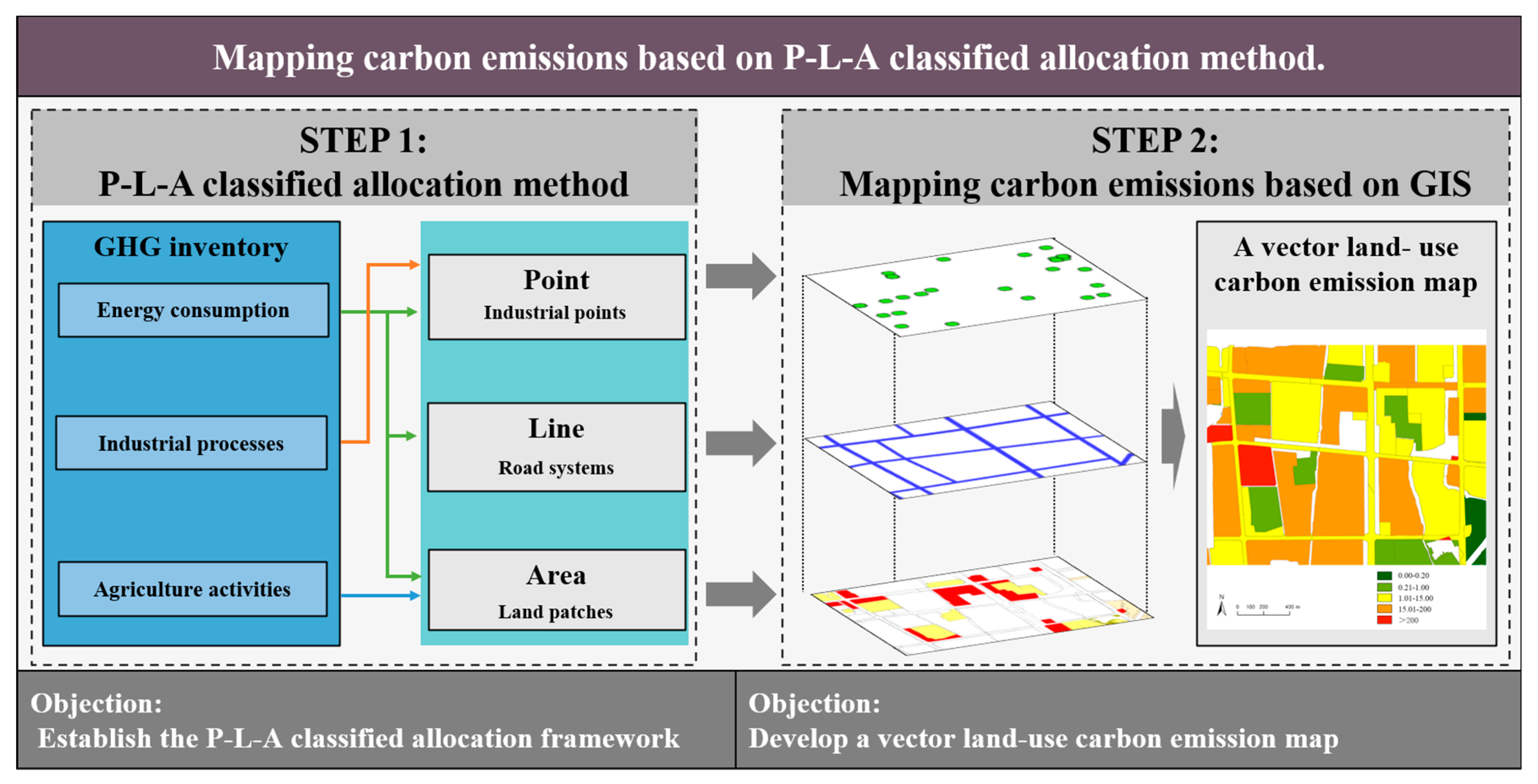
The research method is based on the spatial allocation of carbon emissions of GHG inventory. The basic procedure for the decomposition of the total carbon emissions is comprised of two steps. They are illustrated in the schematic diagram of Figure 1, and the specific explanation is as follows.

In the first step, referring to the studies of Bun et al. [28], Xu [43], and Tang et al. [44] on emission source characteristics of GHG inventory, the carbon emission sources are divided into point, line, and area types. Different algorithms are conducted based on the carbon emission influencing factors as allocation parameters. In this way, a systematic framework for allocating the GHG inventory emissions to three basic objects is established. It is also called the P-L-A carbon emission classified allocation framework. In the second step, a vector database is constructed as the basis of the spatial allocation of GHG inventory emissions. Using the method proposed in the first step, the carbon emissions are allocated to the three types of basic objects and a vector land-use carbon emission map is developed by spatially corresponding the basic objects to land patches based on a geographic information system (GIS).

2.2.1. Step 1: P-L-A Carbon Emission Classified Allocation Method

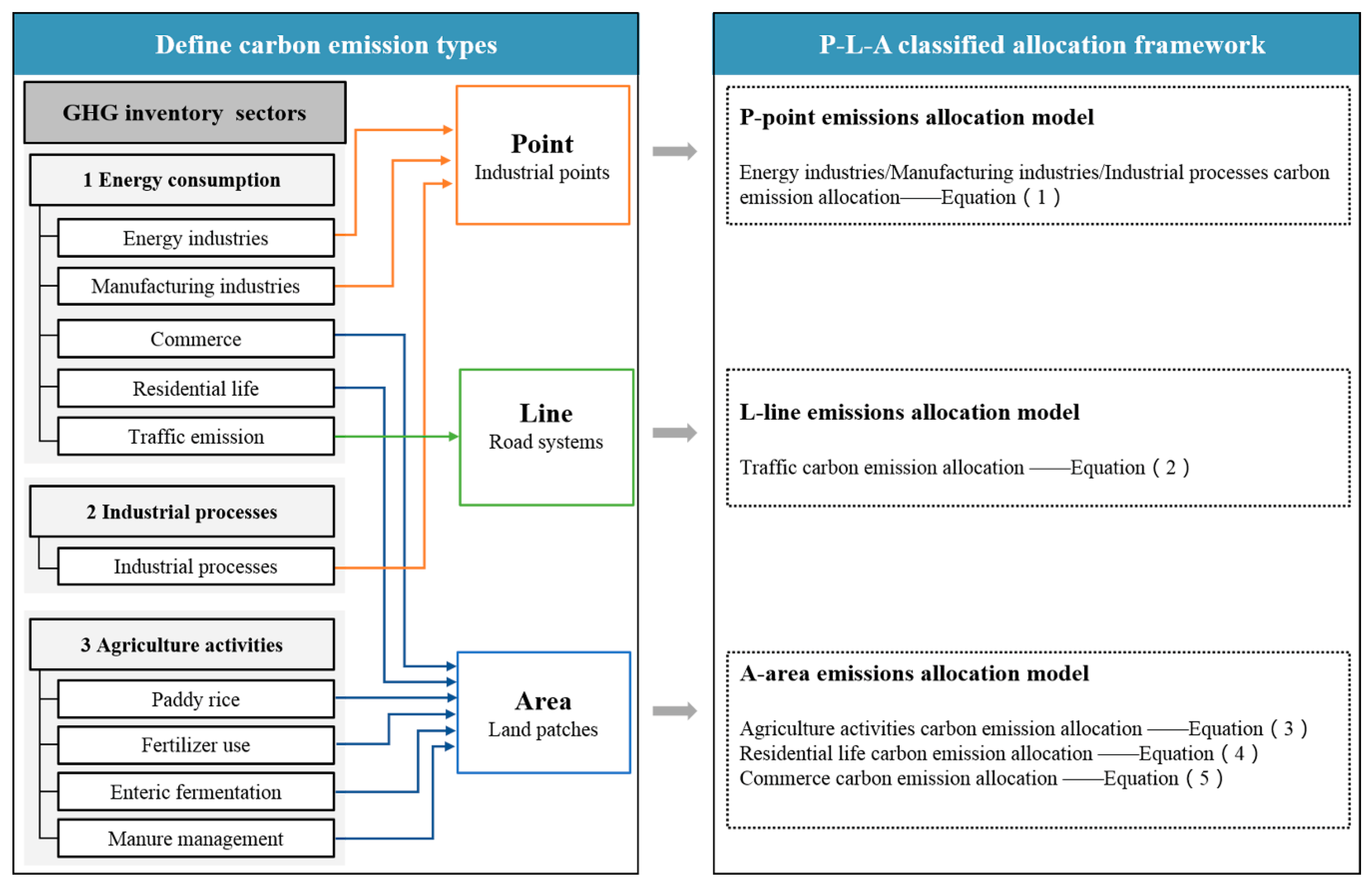
Figure 2 shows the P-L-A carbon emission classified allocation framework. Three major sectors of the five emission sectors of the GHG inventory that the Intergovernmental Panel on Climate Change (IPCC) has defined were considered in this research: energy consumption, industrial processes, and agriculture activities. The principle of this framework is to first classify emission sources as point, line, and area types, and then create classified allocation algorithms for the disaggregation of these emissions to the vector basic objects. The classification of carbon emission sources is based on the emission characteristics of each sector of GHG inventory. For example, industrial carbon emissions have a fixed geographic location, and industrial POI can be easily obtained from the website. These carbon emissions are defined as point type. Carbon emissions from vehicles are not realistic to monitor each car. Therefore, the roads are considered as the emission sources and they are defined as line type. Other emissions from residential life, commerce, and agriculture activities are defined as area type because they are usually calculated for carbon emissions by area. These area emission sources include arable land patches, urban residential land patches, rural settlement land patches, commercial land patches, and public administration and service land patches. The algorithms can be a mathematical model of primary or secondary allocation to decompose the total carbon emissions of each sector of the GHG inventory. Single index or multiple index parameters are selected according to the characteristics of different emission sources to calculate the allocation weight.

Point Emissions Allocation Model

Carbon emissions from energy industries, manufacturing industries, and industrial processes are defined as point emission sources. According to the enterprise directory (ED) [45], the POI information of all enterprises can be obtained through Baidu Map and other online channels. These POI points have accurate latitude and longitude coordinates, which can be used as the basic objects for spatial allocation. Figure 3 shows the procedure of allocating carbon emissions from point sources to the POI points of each enterprise according to the weight of energy production, energy consumption, or output. The mathematical formula for point emissions allocation is shown in Equation (1).

$$C_{ij}=C_{ej}\times \frac{E_{ij}}{E_j}+C_{pj}\times \frac{P_{ij}}{P_j}$$

(1)

where $C_{ij}$ is the carbon emissions of enterprise i of industry j, $C_{ej}$ is the total carbon emissions of industry j from energy production or energy consumption, $C_{pj}$ is the total carbon emissions of industry j from industrial process, $E_{ij}$ is the energy production or energy consumption of enterprise i of industry j, $E_j$ is the total energy production or energy consumption of industry j, $P_{ij}$ is the output of enterprise i of industry j, $P_j$ is the total output of industry j. If there are no industrial process emissions, the $C_{pj}$ will be zero, which means we would only need to allocate the emissions caused by energy production and energy consumption refers to $C_{ej}$.

Line Emissions Allocation Model

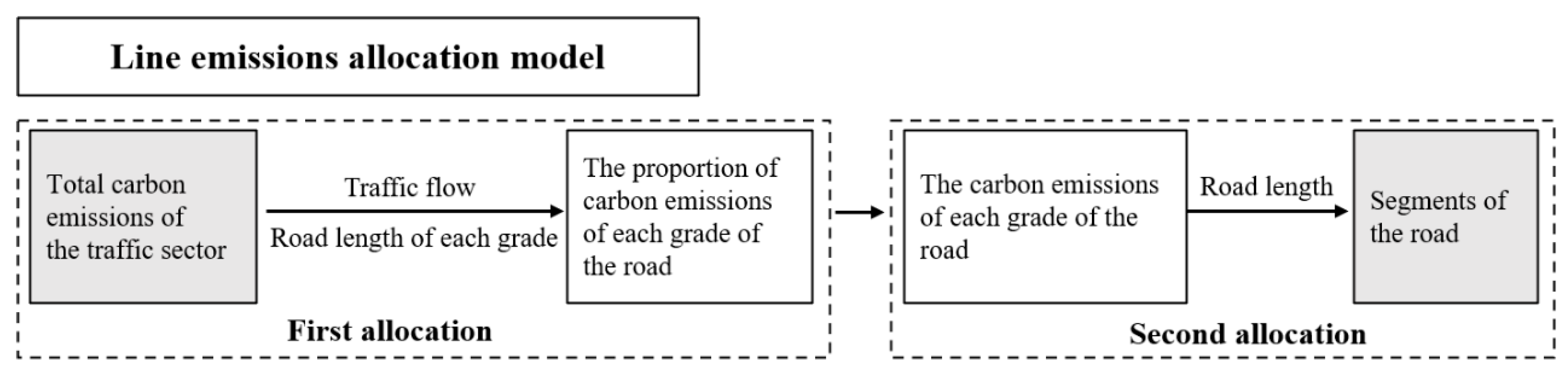
Road systems represent examples of line emission sources. The IPCC stipulates the carbon emissions per unit of vehicle mileage. Since the carbon emissions of line sources mainly depend on the number of vehicles and the driving distances, the carbon emission can be estimated by calculating the total driving distance, which is the product of the two. It is believed that the number of vehicles directly depends on the traffic flow, and the latter depends on the grade of the road. Therefore, a secondary allocation model is used to decompose line emissions to each segment of the road, as shown in Figure 4.

The process of secondary allocation is as follows. First, the proportion of carbon emissions of each grade of the road is calculated according to the traffic flow and road length of different grade of the road. Second, according to the weight of the road length, the carbon emissions of each grade of the road are allocated to each segment. The mathematical formula for line emissions allocation is shown in Equation (2). Road grade classification is divided into national road, provincial road, county road, township road, village road, and urban road according to relevant Chinese standards. The traffic flow data of different grades of the road shown in

Table 1. The reference value of the traffic flow of each grade of the road [46].

Road Grade	National Road	Provincial Road	County Road	Township Road	Village Road	Urban Main Road	Urban Secondary Road	Urban Branch Road
Traffic Flow (Standard vehicles per hour)	4500	1500	1000	1100	500	2800	2600	1100

were obtained from the existing literature [44] and the Comprehensive Traffic Plan of Changxing county.

$$\{\begin{array}{c}{C}_{ij}=C\times {\delta }_j\times \frac{L_{ij}}{L_j}\\ {\delta }_j=\frac{Q_j\times L_j}{{{\displaystyle \sum }}_{j=1}^n(Q_j\times L_j)},\left(n=8\right)\end{array}$$

(2)

where $C_{ij}$ is the carbon emissions of segment i of the road grade j,$C$ is the total carbon emissions of the road system, ${\delta }_j$ is the proportion of carbon emissions in total traffic emissions of grade j, $L_{ij}$ is the length of segment i of road grade j, $L_j$ is the total length of road grade j, $Q_j$ is the traffic flow of road grade j.

Area Emissions Allocation Model

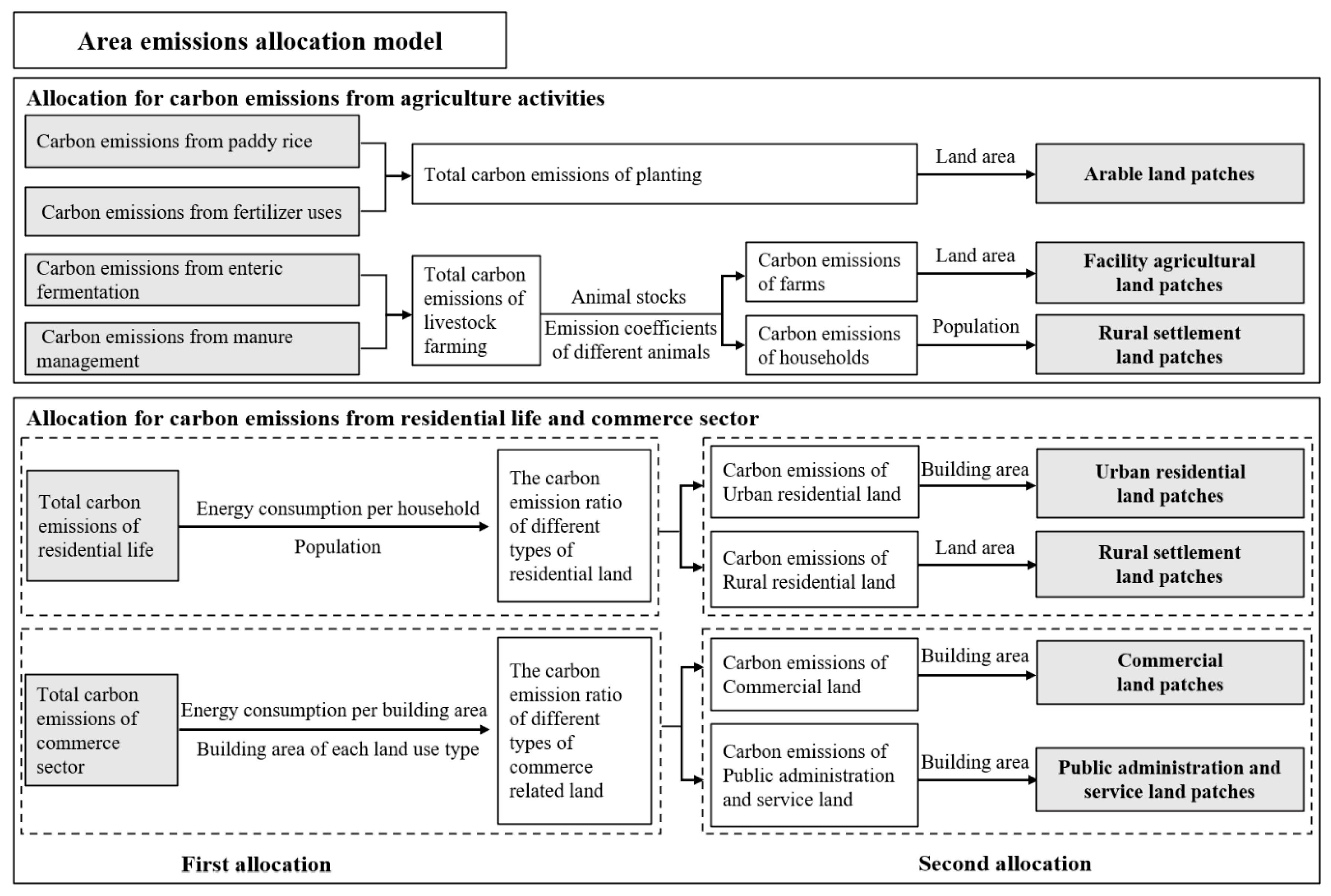
Area emission sources are agricultural activities, commerce, and residential life, and these emissions are allocated to land patches such as arable land, facility agricultural land, urban residential land, rural settlement, commercial land, and public administration and service land. Figure 5 shows the procedure of allocating carbon emissions from area sources to the land patches. The mathematical formulas for area emissions allocation are shown in Equations (3)–(5).

Agricultural activities emitting carbon emissions include paddy rice, fertilizer uses, enteric fermentation, and manure management. The total emissions of the first two are seen as planting emissions, and these emissions are allocated to the arable land patches according to land area weight. The total carbon emissions of the latter two are seen as livestock farming emissions, and these emissions are allocated to the facility agricultural land and rural settlements based on multiweight factors such as animal stocks data (from local statistics, and these data are given separately for farms and households), animal emission coefficients, land area, and population density of rural settlements. Equation (3) shows the algorithm for the allocation of carbon emissions from agricultural activities.

The principles for the allocation of carbon emissions from the residential and commercial sectors are similar. They both use a secondary allocation method for area emissions distribution. First, the carbon emission ratio of different land use is calculated according to the household energy consumption or energy consumption standards per unit building area (

Table 2. The reference values of the energy consumption standards of different buildings.

Building Types	Reference Values of Energy Consumption	Data Sources
Urban housing	2848.53 kWh/household	The reference values of household energy consumption [47]
Rural housing	2160.36 kWh/household
Commercial Office	70 kWh/m2	The standard for the energy consumption of building (GB/T 51161-2016). China. 2016. [48]
Hotel	115 kWh/m2
Shopping mall	130 kWh/m2
Public office	55 kWh/m2

). Then, the carbon emissions of each type of land use are allocated to the corresponding land patches according to the weight of the building area or land area. Equations (4) and (5) show the algorithms for the allocation of carbon emissions from residential life and commerce sector.

$$\{\begin{array}{c}{C}_i=(C_P+C_F)\times \frac{A_i}{{\displaystyle \sum }{A}_i}\\ C_j=(C_E+C_M)\times \sigma \times \frac{A_j}{{\displaystyle \sum }{A}_j}\\ \sigma =\frac{{{\displaystyle \sum }}_{x=1}^n(N_x\times {\mu }_x)}{{{\displaystyle \sum }}_{x=1}^n(N_x\times {\mu }_x)+{{\displaystyle \sum }}_{x=1}^n(Q_x\times {\phi }_x)}\\ C_k=(C_E+C_M)\times \left(1-\sigma \right)\times \frac{P_k}{{\displaystyle \sum }{P}_k}\end{array}$$

(3)

where $C_i$ is the carbon emissions of land patch i of arable land, $C_j$ is the carbon emissions of land patch j of facility agriculture land, $C_k$ is the carbon emissions of land patch k of rural settlement, $C_P$ is the total carbon emissions of paddy rice, $C_F$ is the total carbon emissions of fertilizer uses, $C_E$ is the total carbon emissions of enteric fermentation, $C_M$ is the total carbon emissions of manure management, $A_i$ is the land area of land patch i of arable land, $A_j$ is the land area of land patch j of facility agricultural land, $N_x$ is the animal stocks of farms, ${\mu }_x$ is the animal carbon emission coefficients of farms, $Q_x$ is the animal stocks of households, ${\phi }_x$ is the animal carbon emission coefficients of households, $P_k$ is the population of land patch k of rural settlement.

$$\{\begin{array}{c}{C}_i=C\times \alpha \times \frac{S_i}{{\displaystyle \sum }{S}_i}\\ \alpha =\frac{E_i\times P_i}{E_i\times P_i+E_j\times P_j}\\ C_j=C\times (1-\alpha )\times \frac{A_j}{{\displaystyle \sum }{A}_j}\end{array}$$

(4)

where $C_i$ is the carbon emissions of land patch i of urban residential land, $C$ is the total carbon emissions of residential life,$\alpha$ is the proportion of carbon emissions from urban residential land in total residential life emissions, $S_i$ is the building area of land patch i of urban residential land, $E_i$ is the reference value of energy consumption per household in urban housing, $E_j$ is the reference value of energy consumption per household in rural housing, $P_i$ is urban population, $P_j$ is rural population, $C_j$ is the carbon emissions of land patch j of rural settlement, $A_j$ is the land area of land patch j of rural settlement.

$$\{\begin{array}{c}{C}_i=C\times \beta \times \frac{S_i}{{\displaystyle \sum }{S}_i}\\ \beta =\frac{E_{\beta }\times {\displaystyle \sum }\begin{array}{c}{S}_i\end{array}}{E_{\beta }\times {\displaystyle \sum }{S}_i+E_{\gamma }\times {\displaystyle \sum }{S}_j}\\ E_{\beta }=\frac{E_m\times S_m+E_n\times S_n+E_o\times S_o}{S_m+S_n+S_o}\\ C_j=C\times (1-\beta )\times \frac{S_j}{{\displaystyle \sum }{S}_j}\end{array}$$

(5)

where $C_i$ is the carbon emissions of land patch i of commercial land; $C$ is the total carbon emissions of commerce sector; $\beta$ is the proportion of carbon emissions from commercial land in total commerce sector emissions; $S_i$ is the building area of land patch i of commercial land; $E_{\beta }$ is the energy consumption coefficient per building area of commercial land; $E_m$, $E_n$, and $E_o$ are the reference values of energy consumption per building area of commercial office, hotels, and shopping malls; $S_m,S_n,S_o$ are the respective building areas; $E_{\gamma }$ is the energy consumption coefficient per building area of public administration and service land, which equals the reference value of public office; $S_j$ is the building area of land patch j of public administration and service land; $C_j$ is the carbon emissions of land patch j of public administration and service land.

2.2.2. Step 2: Mapping Carbon Emissions Based on GIS

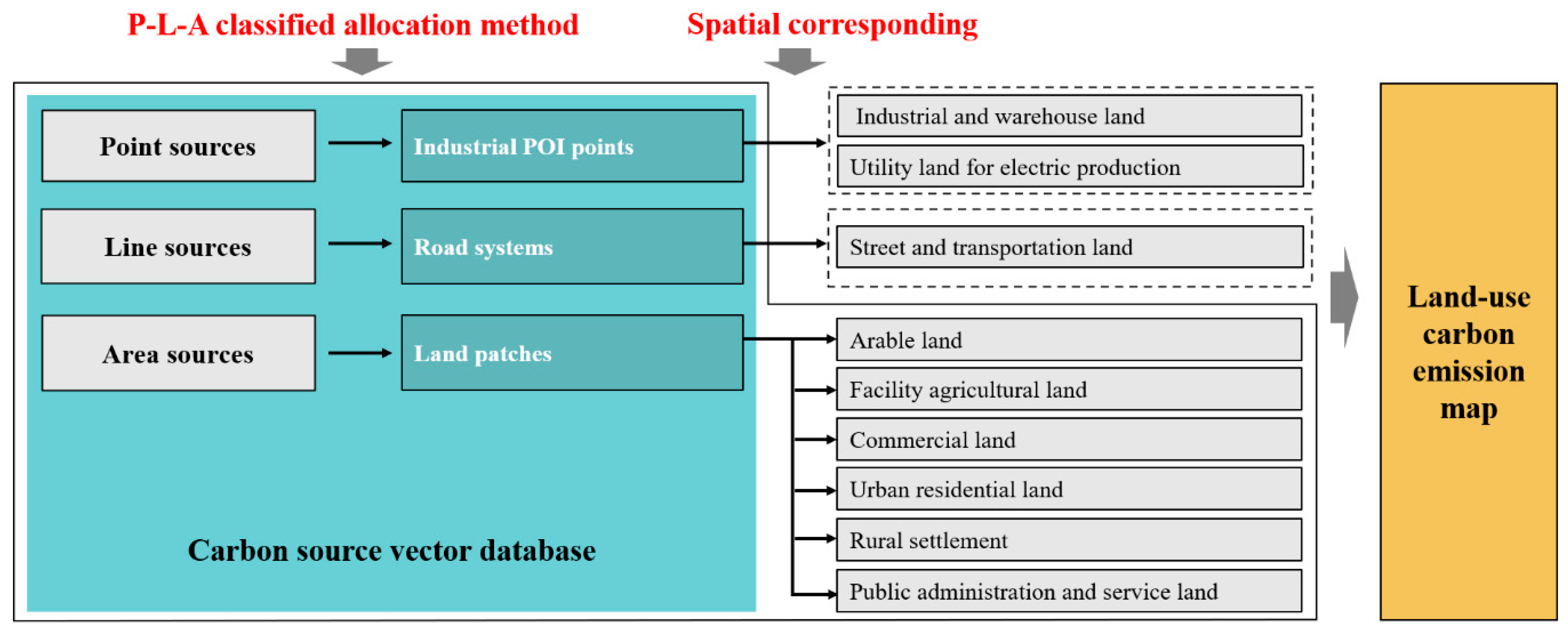
In the process of mapping land-use carbon emissions, a carbon source vector database is first constructed on GIS as the basis for applying the P-L-A carbon emission classified allocation method. As shown in Figure 6, the database is divided into three parts: point sources, line sources, and area sources. Each database contains the basic objects of the emission sources, as well as the detailed allocation parameter information. These data can be obtained from multiple sources, such as local departmental surveys or Internet open-source data, see

Table 3. The description of raw data sources for the carbon source database.

Raw Data	Sources	Data Type
Land use map of Changxing county in 2017	Planning Bureau of Changxing	Vector
Topographic map of Changxing county	Land and Resources Bureau of Changxing	Vector
Industrial POI data	Baidu Map, X-geocoding	Vector
Road systems of Changxing county	Transportation Bureau of Changxing	Raster
The town-level population of Changxing, including the number of households, urban population, rural population, and total population	Public Security Bureau of Changxing	Statistical
Value increased of industrial GDP (10 thousand yuan), energy consumption per industrial increased value (standard coal/10 thousand yuan), emission factors of standard coal (2.773), industrial output data, and industrial energy consumption data	2018 Changxing Statistical Yearbook, The Development and Reform Commission of Changxing	Statistical
Animal stocks data (provided separately by farms and households)	The Agriculture Bureau of Changxing	Statistical

. All data are converted to vector data and adjusted to the same coordinate. Then, the P-L-A carbon emission classified allocation method is used to spatially allocate the carbon emissions of the GHG inventory to the three basic objects: industrial POI points, road systems, and land patches.

Finally, a land-use carbon emission map is constructed by spatially corresponding the point and line emissions to the land patches based on GIS. The land use classification is based on the current land use classification [49] published by the Ministry of Land and Resources of China in 2017, and the Code for classification of urban and rural land use and planning standards of development land [50] published by the Ministry of Housing and Urban–Rural Development of China in 2011. There are nine types of land use that contain carbon emissions. As shown in Figure 6, the industrial POI points correspond to the utility land for electric production or industrial and warehouse land. The road systems correspond to the street and transportation land. In this way, the distribution of carbon emissions from the nine types of land use is realized. Based on GIS spatial statistics, the carbon emission intensity of each land patch is calculated following Equation (6), and the land-use carbon emission intensity map is obtained.

$${\sigma }_i=E_i/A_i$$

(6)

where $E_i$ is the total carbon emissions of land patch i, $A_i$ is the land area of land patch i, ${\sigma }_i$ is the carbon emission intensity of land patch i.

3. Results

3.1. Carbon Source Vector Database

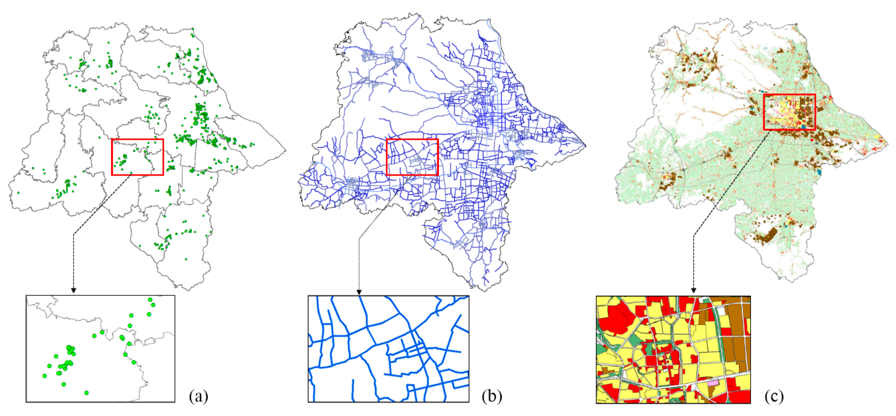
A carbon source vector database of Changxing was constructed on GIS according to the data this method required. The database contained three types of basic objects and all factors that were related to the spatial allocation of carbon emissions, see Figure 7.

(1) The basic objects of the point sources refer to POI points of energy and industrial enterprises. The 618 POI points in Changxing were obtained through X-geocoding and Baidu Map, including latitude and longitude information, as well as the industry classification. These industrial POI points were used to allocate carbon emissions from the point sources.

(2) The basic objects of the line sources refer to the road systems based on the comprehensive traffic plan of Changxing and Baidu Map. These lines contain information such as road grade, traffic flow, and length of each segment, which were used to allocate the traffic emissions.

(3) The basic objects of the area sources refer to land patches of six land use types. The complete land-use database contained nine types of carbon source land, which was established by integrating the data of remote-sensing imagery, digitalized land-use maps of urban planning, and vector land use map from the local government. By spatial connection of GIS, each land patch was endowed with attribute information such as land area, building area, administrative attributes, population density, etc., which can be used for the spatial allocation of carbon emissions of agricultural activities, commerce, and residential life to the related land patches.

3.2. Vector Carbon Emission Map Based on Land Patches

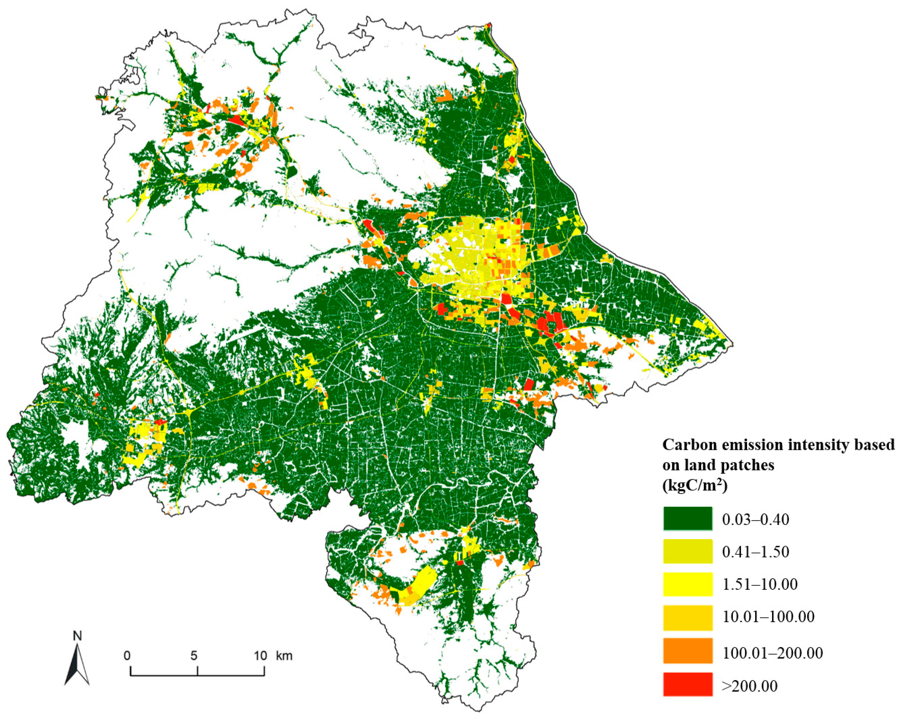
Based on the carbon source vector database, the P-L-A classified allocation method was used to allocate the carbon emissions of the main sectors of the 2017 GHG inventory of Changxing to the three types of basic objects. The results were further related to the nine types of carbon source land patches through GIS.

Table 4. The correspondence between the carbon emissions of greenhouse gas (GHG) inventory and land use types in Changxing.

GHG Inventory Sector	Source Type	Basic Objects	Corresponding Land Use Types
Energy Consumption
Electric industries	Point source	13 POI points of electric industries	Utility land for electric production
Manufacturing industries	Point source	605 POI points of different industries	Industrial and warehouse land
Commerce	Area source	Commercial land patches, public administration, and service land patches	Commercial land, public administration, and service land
Residential life	Area source	Residential land patches	Urban residential land, Rural settlement
Traffic emission	Line source	Road systems	Street and transportation land
Industrial Process
Cement industry	Point source	8 POI points of cement industries	Industrial and warehouse land
Lime industry	Point source	3 POI points of lime industries	Industrial and warehouse land
Agriculture Activities
Paddy rice	Area source	Arable land patches	Arable land
Fertilizer use	Area source	Arable land patches	Arable land
Enteric fermentation	Area source	Facility agricultural land patches, rural settlement land patches	Facility agricultural land, Rural settlement
Manure management	Area source	Facility agricultural land patches, rural settlement land patches	Facility agricultural land, Rural settlement

shows the correspondence between the carbon emissions of GHG inventory sectors and the nine types of land use. Figure 8 shows the carbon emission intensity map based on land patches of Changxing. The detailed carbon emission data of 85,911 land patches in Changxing county can be found in Table S1 of the Supplementary Materials.

As can be seen from Figure 8, the results of the land-use carbon emissions show considerable unevenness in the spatial distribution. The high-intensity areas are concentrated in the city center and four industrial towns located in the northwest and east. This shows that carbon emissions mainly come from urban life and industrial energy consumptions. The industrial sector has the most carbon emissions.

From the perspective of land use, there are significant differences in the carbon emission intensity of detailed land use types. The highest intensity land uses are mainly the utility land for electric production, the industrial and warehouse land, and the street and transportation land, with an average intensity above 100 kgC/m². Followed by the facility agriculture land, the commercial land, and the public administration and service land, the average intensity is between 1.51–10 kgC/m². Buildings on commercial land, such as shopping malls, hotels, and business offices have huge energy consumptions, so the carbon emission intensity of commercial land is significantly higher than that of the public administration and service land mainly for administrative offices, education, and scientific research. The average carbon emission intensity of residential land is less than 10 kgC/m². The average carbon emission intensity of urban residential land is about eight times higher than that of rural settlement. Although the carbon emission intensity of arable land is small, the total emissions account for a relatively high proportion due to the large area of Arable land.

3.3. Cross Comparison with Existing Methods

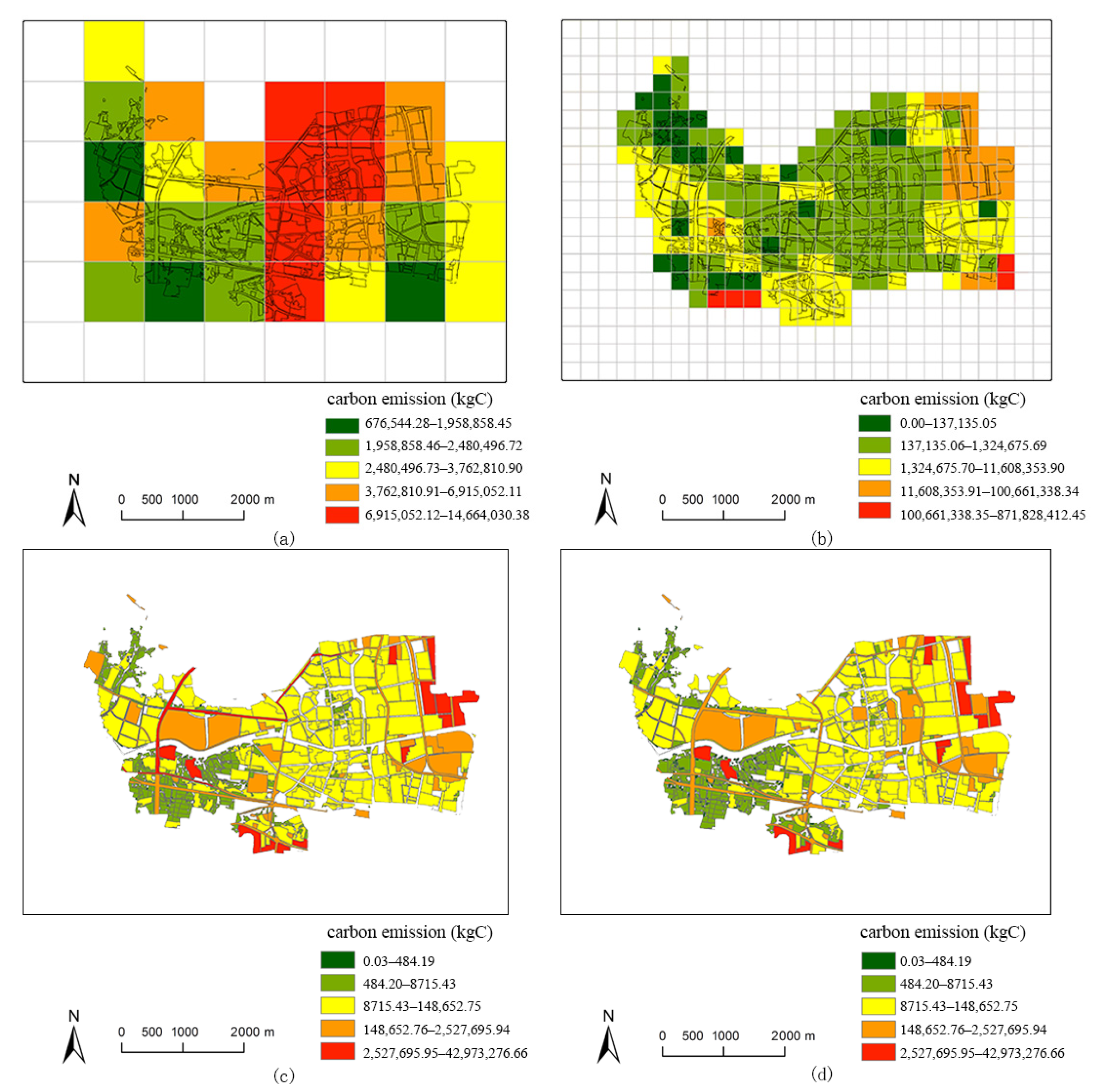
The results of this study were compared with the mapping results from replicating three other methods [9,32,51], taking Zhicheng town in Changxing for example. All mappings were based on the same total carbon emission data provided by the 2017 GHG inventory of Changxing. The detailed allocation information of each method is shown in

Table 5. Detailed allocation information of the four carbon emission mapping methods.

Method	Allocation Weight	Basic Objects	Map Type	Method Source
I	Single-weight: population density	1 km × 1 km grid	Gridded map	CDIAC [51]
II	Multiweight: land area, GDP, population, building area, industry categories, etc.	300 m × 300 m grid	Gridded map	Chuai et al. [32]
III	Single-weight: land use type	Land patches	Vector map	Zhang et al. [9]
IV	Multiweight: energy consumption data, land area, population, building area, traffic flow, road length, industry categories, industry output, etc.	P: Industrial POI points L: Road systems A: Land patches	Vector map	P-L-A classified allocation method proposed by this study

. This comparison shows that the estimation results obtained by this method are more accurate at the land patch level.

As shown in Figure 9, by comparing with the carbon emission maps by different methods, the advantages of the vector carbon emission mapping method in the spatial resolution are revealed. In general, the four maps show similar spatial distribution as high carbon emissions in the east and west and low carbon emissions in the middle. This may be related to a large amount of industrial land in the east and west districts. However, compared with gridded maps shown in Figure 9a,b, the following two vector carbon emission maps provide the carbon emission of land patches with clear geographical location and boundaries, which can provide a more intuitive support for urban planning. The main difference between Figure 9c,d is the identification of the high carbon emission land patches in the middle area, which happens to be the commercial center or residential center of the region. Through actual investigation, it was found that these land patches have high energy consumption and carbon emissions, which is more consistent with the results of our method.

Table 6. The carbon emission ratios of different land use types by the four methods.

Land Use Type	Method I	Method II	Method III	Method IV
Urban residential land	27.20%	23.28%	3.03%	3.40%
Rural settlement	12.59%	11.16%	0.44%	0.08%
Commercial land	19.08%	5.58%	2.09%	3.28%
Administration and service land	11.39%	3.18%	1.99%	0.79%
Industrial and warehouse land	4.98%	17.11%	82.82%	82.82%
Street and transportation land	6.04%	10.48%	9.26%	9.26%
Arable land	18.72%	29.20%	0.36%	0.36%
Total carbon emissions (kgC)	180.13 × 106	180.13 × 106	180.13 × 106	180.13 × 106

shows the carbon emission ratios of different land use types by the four allocation methods. There are significant differences in the proportion of carbon emissions from different land use obtained by the decomposition of the same total carbon emissions. Different from method I and II, in the vector carbon emission mapping results of method III and IV, carbon emissions of the industrial and warehouse land account for more than 80% of the total emissions, which is more consistent with the existing research and actual situation. It reflects that the vector carbon emission maps are more accurate than the gridded maps in estimating land patch carbon emissions.

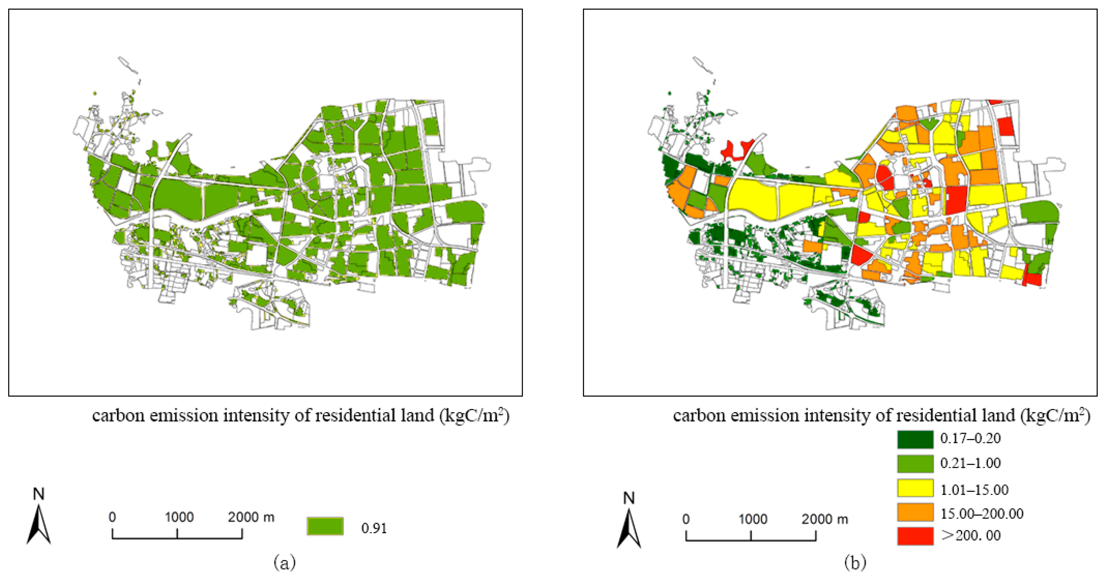
We further compared the carbon emission intensity distribution of the same type of land use in method III and IV. Taking residential land as an example, Figure 10a,b show the carbon emission intensity distribution of residential land. It can be seen that our method, IV, is more effective in identifying the internal differences of the same land use type. This is very helpful for explaining the differences between urban and rural areas and the differences in other detailed land use types caused by building function, building scale, plot ratio, and other factors.

To sum up, different from the previous allocation methods, the approach proposed in this paper takes into account the influencing factors of different types of carbon emissions. The P-L-A classified allocation method based on multiweight can make the mapping results more consistent with the actual situation. It can better identify differences in carbon emissions of detailed land use types and more accurately estimate the carbon emissions of each land patch.

4. Discussion

4.1. Application of the Map at the City Scale and Land Patch Scale

In recent years, how to accurately allocate and visualize the overall carbon emissions to each land patch has been a great concern [52,53,54]. The method proposed in this paper can be used to construct a vector land-use carbon emission map for a city that has compiled the GHG inventory. The emission map can enable the display of the real contributions of each land patch to the overall emissions. This is of significant effect in guiding urban carbon emission reduction policy and low-carbon planning. Taking Changxing as a case study, the detailed applications are shown in the following two aspects.

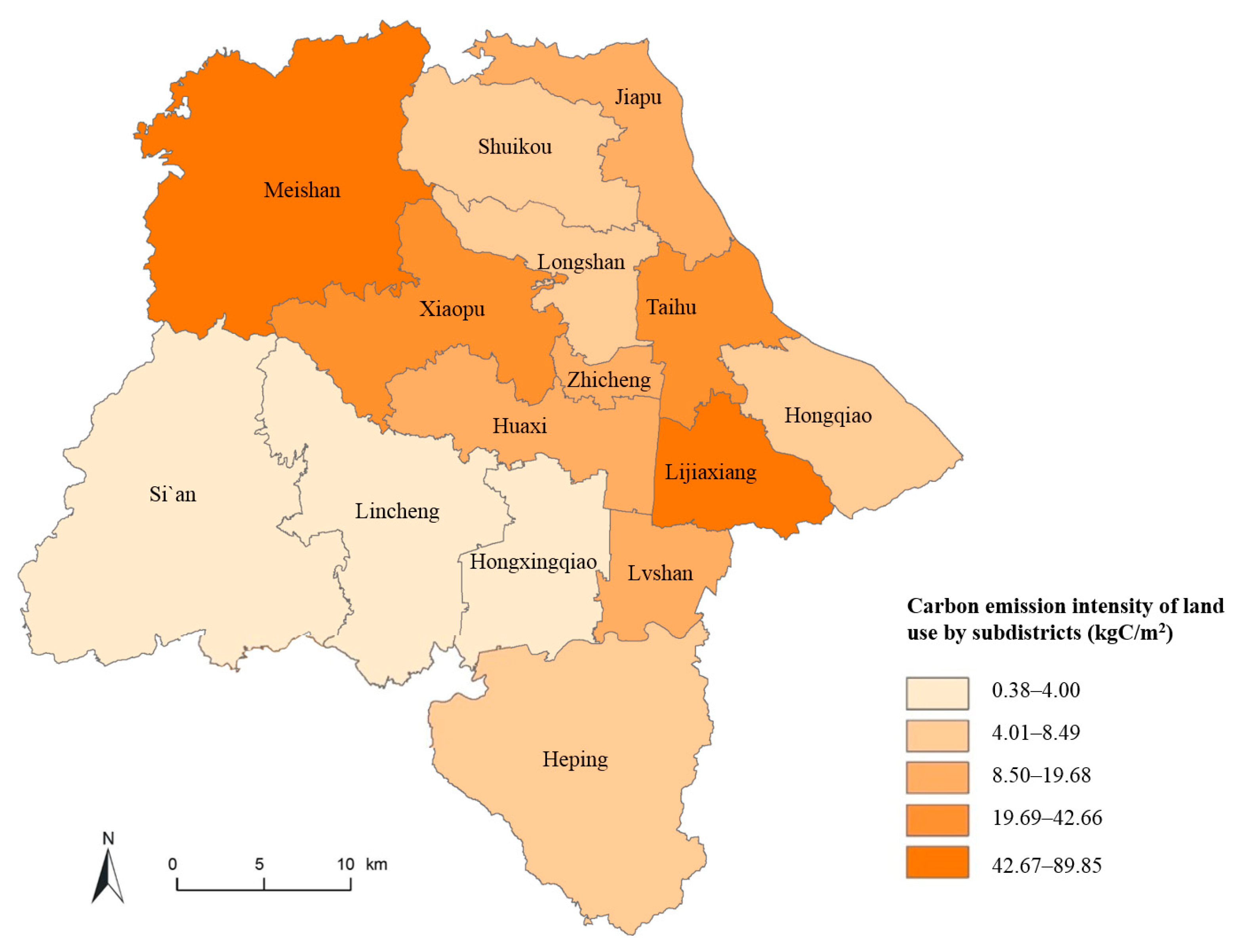
For one thing, the total emissions can be calculated for any administrative unit at the level of city/county, subdistrict/town, or community/village without any loss of accuracy. The results can provide more accurate information for the local government’s carbon emission control and management. Specific applications of the carbon emission map include identifying the key carbon emission administrative districts or guiding the decomposition of regional emission reduction targets into basic administrative units, such as subdistricts or towns. Figure 11 shows the total carbon emissions of 15 subdistricts in Changxing. The towns with the highest land-use carbon emission intensity are Meishan and Lijiaxiang, with the carbon emission intensity exceeding 60 kgC/m²; the following are Xiaopu and Taihu, with an intensity of about 35 kgC/m²; the lowest is Si’an, Shuikou, and other towns, with an intensity value less than 5 kgC/m². The study found that the four towns with higher carbon emission intensity are also important industrial towns in Changxing. These towns are the focus of Changxing’s efforts to reduce carbon emissions by adjusting the industrial structure or improving energy efficiency. According to the proportion of carbon emissions, they should be responsible for about 80% of the overall carbon reduction target of Changxing.

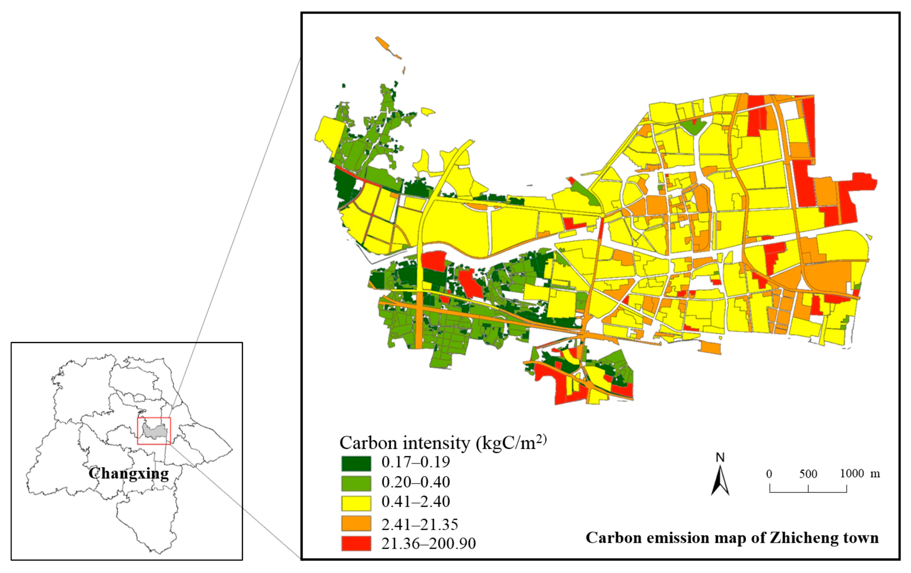
For another thing, the vector land-use carbon emission map can provide carbon emissions of each land patch, as well as land patch-level emission impact factors. This is very essential for low-carbon planning as the map permits the visualization of how and why existing land patches affect the carbon emissions due to their function, form, density, and other indicators. Existing studies have proved the important effects of land use types, building density, floor area ratio, etc. on carbon emissions [5,55,56,57,58]. However, the quantitative relationship and internal mechanisms between them are still unclear [59,60]. The vector carbon emission map provides enough data for our further study of the relationship between carbon emissions and the internal characteristics of land use. For example, Figure 12 contains more than 800 land patches with the carbon emission intensity information in Zhicheng town. At the same time, the characteristic indicators of land patches can also be obtained based on the carbon source database, such as land use type, land area, floor area ratio, building height, building density, etc. These data can support further research to quantify the relationship between carbon emissions and the characteristics of land use at a detailed scale, thereby providing additional support for urban planning to achieve carbon reduction through land patch control.

4.2. Limitations and Further Improvements

There are also some uncertainties and shortcomings of the P-L-A carbon emission classified allocation method. First, there may be some position deviation when the industrial POI points or road systems correspond to related land patches. Second, when allocating carbon emissions from the residential life and commerce sector, this research assumes that all floors of the same type of land use are in use and that the same type of building has the same energy consumption level based on related research and standards, which may contrast with reality to some extent.

Further studies should consider all land-use types in the entire region, with particular attention to the detailed land use types in urban areas that contain major human activities. According to the carbon emission characteristics of different land uses, more precise parameters and allocation algorithms are required. This process will involve large field investigations to improve the accuracy of the spatial allocation method.

5. Conclusions

In this paper, a vector mapping method of carbon emissions based on the P-L-A classified allocation framework was presented. It establishes the relationship between the GHG inventory and a vector carbon emission map. The method includes two steps: establishing the P-L-A carbon emission classified allocation framework based on the classification of different carbon sources of GHG inventory and mapping carbon emissions by corresponding the emissions of basic objects to land patches based on GIS. Changxing county was taken as a case study to apply the method. Some conclusions can be obtained as follows.

(1) The carbon emission map conducted by this method can accurately identify the key emission regions. The carbon emission map of Changxing shows that high-intensity areas are concentrated in four industrial towns (accounting for about 80%) and the central city. These four industrial towns should assume the main responsibility of the entire carbon reduction target.

(2) This method can better identify differences in carbon emissions of detailed land-use types. The highest carbon emission intensity in Changxing is the utility land for electric production, the industrial and warehouse land, and the street and transportation land. This is followed by the facility agricultural land, the commercial land, and the public administration and service land. The carbon emission intensity of residential land is less than the former. Furthermore, this method could calculate in more detail that the average carbon emission intensity of urban residential land is about eight times that of rural settlement.

(3) Compared with the other three carbon emission mapping methods, it is verified that this method is more accurate in estimating land patch-level carbon emissions, and the estimation results are more consistent with the actual situation.

The vector carbon emission map conducted by the method this paper proposed can provide valuable guidance for emission reduction policies and low-carbon planning. For the government, calculating the carbon emissions of each administrative unit based on the carbon emission map can identify the key carbon reduction regions. For urban planners, it can provide an accurate estimation of carbon emissions and other internal characteristics of each land patch, which can be an additional support for urban planning to achieve carbon reduction.

References

- Bulkeley, H. A changing climate for spatial planning. Plan. Theory Pract. 2006, 7, 203–214. [Google Scholar] [CrossRef]
- Marcotullio, P.J.; Sarzynski, A.; Albrecht, J.; Schulz, N.; Garcia, J. Assessing Urban Greenhouse Gas Emissions in European Medium and Large Cities: Methodological Considerations. In Sustainable Cities: Assessing the Performance and Practice of Urban Environments; I.B. Tauris & Co. Ltd.: London, UK, 2016; pp. 83–101. [Google Scholar]
- Khan, F.; Pinter, L. Scaling indicator and planning plane: An indicator and a visual tool for exploring the relationship between urban form, energy efficiency and carbon emissions. Ecol. Indic. 2016, 7, 183–192. [Google Scholar] [CrossRef] [Green Version]
- Wang, S.H.; Huang, S.L.; Huang, P.J. Can spatial planning really mitigate carbon dioxide emissions in urban areas? A case study in Taipei, Taiwan. Landsc. Urban Plan. 2018, 1696, 22–36. [Google Scholar] [CrossRef]
- Hargreaves, A.; Cheng, V.; Deshmukh, S.; Leach, M.; Steemers, K. Forecasting how residential urban form affects the regional carbon savings and costs of retrofitting and decentralized energy supply. Appl. Energy 2017, 186, 549–561. [Google Scholar] [CrossRef] [Green Version]
- Zhao, J.; Thinh, N.X.; Li, C. Investigation of the impacts of urban land use patterns on energy consumption in China: A case study of 20 provincial capital cities. Sustainability 2017, 9, 1383. [Google Scholar] [CrossRef] [Green Version]
- Gately, C.K.; Hutyra, L.R.; Wing, I.S.; Brondfield, M.N. A bottom up approach to on-road CO2 emissions estimates: Improved spatial accuracy and applications for regional planning. Environ. Sci. Technol. 2013, 47, 2423–2430. [Google Scholar] [CrossRef]
- Chuai, X.; Huang, X.; Wang, W.; Zhao, R.; Zhang, M.; Wu, C. Land use, total carbon emissions change and low carbon land management in Coastal Jiangsu, China. J. Clean. Prod. 2015, 103, 77–86. [Google Scholar] [CrossRef]
- Zhang, G.; Ge, R.; Lin, T.; Ye, H.; Li, X.; Huang, N. Spatial apportionment of urban greenhouse gas emission inventory and its implications for urban planning: A case study of Xiamen, China. Ecol. Indic. 2018, 85, 644–656. [Google Scholar] [CrossRef]
- Chang, C.T.; Yang, C.H.; Lin, T.P. Carbon dioxide emissions evaluations and mitigations in the building and traffic sectors in Taichung metropolitan area, Taiwan. J. Clean. Prod. 2019, 230, 1241–1255. [Google Scholar] [CrossRef]
- Geertman, S.; Stillwell, J. Planning support systems: An inventory of current practice. Comput. Environ. Urban Syst. 2004, 28, 291–310. [Google Scholar] [CrossRef]
- Gurney, K.R.; Romero-Lankao, P.; Seto, K.C.; Hutyra, L.R.; Duren, R.; Kennedy, C.; Grimm, N.B.; Ehleringer, J.R.; Marcotullio, P.; Hughes, S.; et al. Climate change: Track urban emissions on a human scale. Nature 2015, 525, 179–181. [Google Scholar] [CrossRef] [Green Version]
- Yamagata, Y.; Yoshida, T.; Murakami, D.; Matsui, T.; Akiyama, Y. Seasonal urban carbon emission estimation using spatial micro Big Data. Sustainability 2018, 10, 4472. [Google Scholar] [CrossRef] [Green Version]
- Laine, J.; Heinonen, J.; Junnila, S. Pathways to carbon-neutral cities prior to a national policy. Sustainability 2020, 12, 2445. [Google Scholar] [CrossRef] [Green Version]
- Wang, G.; Han, Q.; de Vries, B. A geographic carbon emission estimating framework on the city scale. J. Clean. Prod. 2020, 244, 1187963. [Google Scholar] [CrossRef]
- Muntean, M.; Janssens-Maenhout, G.; Song, S.; Selin, N.E.; Olivier, J.G.J.; Guizzardi, D.; Maas, R.; Dentener, F. Trend analysis from 1970 to 2008 and model evaluation of EDGARv4 global gridded anthropogenic mercury emissions. Sci. Total Environ. 2014, 494, 337–350. [Google Scholar] [CrossRef]
- Sharifi, A.; Wu, Y.; Khamchiangta, D.; Yoshida, T.; Yamagata, Y. Urban carbon mapping: Towards a standardized framework. Energy Procedia 2018, 152, 799–808. [Google Scholar] [CrossRef]
- Wu, Y.; Sharifi, A.; Yang, P.; Borjigin, H.; Murakami, D.; Yamagata, Y. Mapping building carbon emissions within local climate zones in Shanghai. Energy Procedia 2018, 152, 815–822. [Google Scholar] [CrossRef]
- Horabik, J.; Nahorski, Z. Improving resolution of a spatial air pollution inventory with a statistical inference approach. Clim. Chang. 2014. [Google Scholar] [CrossRef] [Green Version]
- Wang, J.; Cai, B.; Zhang, L.; Cao, D.; Liu, L.; Zhou, Y.; Zhang, Z.; Xue, W. High resolution carbon dioxide emission gridded data for China derived from point sources. Environ. Sci. Technol. 2014, 48, 7085–7093. [Google Scholar] [CrossRef]
- Andres, R.J.; Boden, T.A.; Higdon, D.M. Gridded uncertainty in fossil fuel carbon dioxide emission maps, a CDIAC example. Atmos. Chem. Phys. 2016, 16. [Google Scholar] [CrossRef] [Green Version]
- Andres, R.J.; Marland, G.; Fung, I.; Matthews, E. A 1°× 1°distribution of carbon dioxide emissions from fossil fuel consumption and cement manufacture, 1950–1990. Glob. Biogeochem. Cycles 1996, 10, 419–429. [Google Scholar] [CrossRef]
- Doll, C.N.H.; Muller, J.P.; Elvidge, C.D. Night-time imagery as a tool for global mapping of socioeconomic parameters and greenhouse gas emissions. Ambio 2000, 29, 157–162. [Google Scholar] [CrossRef]
- Ghosh, T.; Elvidge, C.D.; Sutton, P.C.; Baugh, K.E.; Ziskin, D.; Tuttle, B.T. Creating a global grid of distributed fossil fuel CO2 emissions from nighttime satellite imagery. Energies 2010, 3, 1895–1913. [Google Scholar] [CrossRef]
- Oda, T.; Maksyutov, S. A very high-resolution (1km × 1 km) global fossil fuel CO2 emission inventory derived using a point source database and satellite observations of nighttime lights. Atmos. Chem. Phys. 2011, 11, 543. [Google Scholar] [CrossRef] [Green Version]
- Wang, Y. Multi-scale spatial allocation method of Chinese fossil fuel carbon dioxide emission statistics data. Cent. China Norm. Univ. China 2017, 3, 20–27. (In Chinese) [Google Scholar]
- Olivier, J.G.J.; Van Aardenne, J.A.; Dentener, F.J.; Pagliari, V.; Ganzeveld, L.N.; Peters, J.A.H.W. Recent trends in global greenhouse gas emissions:regional trends 1970–2000 and spatial distributionof key sources in 2000. Environ. Sci. 2005, 2, 81–99. [Google Scholar] [CrossRef] [Green Version]
- Bun, R.; Nahorski, Z.; Horabik-Pyzel, J.; Danylo, O.; See, L.; Charkovska, N.; Topylko, P.; Halushchak, M.; Lesiv, M.; Valakh, M.; et al. Development of a high-resolution spatial inventory of greenhouse gas emissions for Poland from stationary and mobile sources. Mitig. Adapt. Strateg. Glob. Chang. 2019, 24, 853–880. [Google Scholar] [CrossRef] [Green Version]
- Wang, R.; Tao, S.; Ciais, P.; Shen, H.Z.; Huang, Y.; Chen, H.; Shen, G.F.; Wang, B.; Li, W.; Zhang, Y.Y.; et al. High-resolution mapping of combustion processes and implications for CO2 emissions. Atmos. Chem. Phys. 2013, 13, 5189–5203. [Google Scholar] [CrossRef] [Green Version]
- Heiple, S.; Sailor, D.J. Using building energy simulation and geospatial modeling techniques to determine high resolution building sector energy consumption profiles. Energy Build. 2008, 40, 1426–1436. [Google Scholar] [CrossRef] [Green Version]
- Cai, B.; Li, W.; Dhakal, S.; Wang, J. Source data supported high resolution carbon emissions inventory for urban areas of the Beijing-Tianjin-Hebei region: Spatial patterns, decomposition and policy implications. J. Environ. Manag. 2018, 206, 786–799. [Google Scholar] [CrossRef]
- Chuai, X.; Feng, J. High resolution carbon emissions simulation and spatial heterogeneity analysis based on big data in Nanjing City, China. Sci. Total Environ. 2019, 686, 828–837. [Google Scholar] [CrossRef]
- Lorenzo-Sáez, E.; Oliver-Villanueva, J.V.; Coll-Aliaga, E.; Lemus-Zúñiga, L.G.; Lerma-Arce, V.; Reig-Fabado, A. Energy efficiency and GHG emissions mapping of buildings for decision-making processes against climate change at the local level. Sustainability 2020, 12, 2982. [Google Scholar] [CrossRef] [Green Version]
- Akiyama, Y. Applications of micro geodata for urban monitoring. In Proceedings of the 16th International Conference on Geographic Information Systems: Spatial Big Data Technologies and Applications for Future Society, Soul, Korea, 16 August 2014; pp. 103–116. [Google Scholar]
- Akiyama, Y.; Nishimoto, Y.; Shibasaki, R. Projecting future distributions of facility deserts for smart regionalplanning: A micro geodata approach in Japan. In Proceedings of the 15th International Conference on Computers in Urban Planning and Urban Management, Adelaide, Australia, 11–14 July 2017; p. 35081. [Google Scholar]
- Dai, S.; Zuo, S.; Ren, Y. A spatial database of CO2 emissions, urban form fragmentation and city-scale effect related impact factors for the low carbon urban system in Jinjiang city, China. Data Br. 2020, 29, 105274. [Google Scholar] [CrossRef]
- Yamagata, Y.; Murakami, D.; Yoshida, T. Urban carbon mapping with spatial Big Data. Energy Procedia 2017, 142, 2461–2466. [Google Scholar] [CrossRef]
- Liu, C.; Wang, T. Identifying and mapping local contributions of carbon emissions from urban motor and metro transports: A weighted multiproxy allocating approach. Comput. Environ. Urban Syst. 2017, 64, 132–143. [Google Scholar] [CrossRef]
- Makido, Y.; Yamagata, Y.; Dhakal, S. Effect of urban forms: Towards the reduction of CO2 emissions. In Proceedings of the American Society for Photogrammetry and Remote Sensing Annual Conference 2010: Opportunities for Emerging Geospatial Technologies, Reno, NV, USA, 23–24 February 2010. [Google Scholar]
- Ma, J.; Liu, Z.; Chai, Y. The impact of urban form on CO2 emission from work and non-work trips: The case of Beijing, China. Habitat Int. 2015, 47, 1–10. [Google Scholar] [CrossRef]
- Fang, C.; Wang, S.; Li, G. Changing urban forms and carbon dioxide emissions in China: A case study of 30 provincial capital cities. Appl. Energy 2015, 158, 519–531. [Google Scholar] [CrossRef]
- China County Economic Development Report (2017); Guangdong Economic Publishing House: Guangdong, China, 2017.
- Xu, S. Carbon Accounting and Space Distribution for the Cities in China-a Case of Nanjing City; Nanjing University: Nanjing, China, 2011; pp. 37–44. (In Chinese) [Google Scholar]
- Tang, X.; Hutyra, L.R.; Arévalo, P.; Baccini, A.; Woodcock, C.E.; Olofsson, P. Spatiotemporal tracking of carbon emissions and uptake using time series analysis of Landsat data: A spatially explicit carbon bookkeeping model. Sci. Total Environ. 2020, 720, 1374096. [Google Scholar] [CrossRef]
- ED. Available online: http://www.trustexporter.com/changxing/ (accessed on 9 May 2017).
- Jing, Y. Carbon Accounting and Spatial Distribution in Nanning Metropolitan Region Based on Land Cover; Guangxi University: Guangxi, China, 2015; pp. 64–65. (In Chinese) [Google Scholar]
- Wang, Y.; Zhao, P. Survey Research on Residential Building Energy Consumption in Urban and Rural Area of China. Beijing Daxue Xuebao (Ziran Kexue Ban)/Acta Sci. Nat. Univ. Pekin. 2018, 1, 162–170. [Google Scholar] [CrossRef]
- Standard for Energy Consumption of Building (GB/T 51161-2016). Available online: http://www.jianbiaoku.com/webarbs/book/87540/2707023.shtml (accessed on 1 December 2020).
- Current Land Use Classification (GB/T 21010-2017). Available online: http://www.tdzyw.com/2017/1113/45597.html (accessed on 1 December 2020).
- Code for Classification of Urban Land Use and Planning Standards of Development LAND (GB/T 50137-2011). Available online: http://max.book118.com/html/2017/0407/99167799.shtm (accessed on 1 December 2020).
- Carbon Dioxide Information Analysis Center (CDIAC). Available online: http://cdiac.ornl.gov/ (accessed on 14 October 2018).
- Abeydeera, L.H.U.W.; Mesthrige, J.W.; Samarasinghalage, T.I. Global research on carbon emissions: A scientometric review. Sustainability 2019, 11, 3972. [Google Scholar] [CrossRef] [Green Version]
- Peters, G.P. Carbon footprints and embodied carbon at multiple scales. Curr. Opin. Environ. Sustain. 2010, 2, 245–250. [Google Scholar] [CrossRef]
- Yang, J.; Zhan, Y.; Xiao, X.; Xia, J.C.; Sun, W.; Li, X. Investigating the diversity of land surface temperature characteristics in different scale cities based on local climate zones. Urban Clim. 2020, 34, 100700. [Google Scholar] [CrossRef]
- Ewing, R.; Rong, F. The impact of urban form on U.S. residential energy use. Hous. Policy Debate 2008, 19, 1–30. [Google Scholar] [CrossRef]
- Qin, B.; Qi, B. The Impact of Urban Form on Household Building Carbon Emission: A Case Study of Beijing. Urban Plan. Int. 2013, 28, 42–46. [Google Scholar]
- Yang, J.; Su, J.; Xia, J.C.; Jin, C.; Li, X.; Ge, Q. The Impact of Spatial Form of Urban Architecture on the Urban Thermal Environment: A Case Study of the Zhongshan District, Dalian. IEEE J. Sel. Top. Appl. Earth Obs. Remote Sens. 2018, 11, 2709–2716. [Google Scholar] [CrossRef]
- Qiao, Z.; Tian, G.; Xiao, L. Diurnal and seasonal impacts of urbanization on the urban thermal environment: A case study of Beijing using MODIS data. ISPRS J. Photogramm. Remote Sens. 2013, 85, 93–101. [Google Scholar] [CrossRef]
- Yang, J.; Jin, S.; Xiao, X.; Jin, C.; Xia, J.; Li, X.; Wang, S. Local climate zone ventilation and urban land surface temperatures: Towards a performance-based and wind-sensitive planning proposal in megacities. Sustain. Cities Soc. 2019, 47, 101487. [Google Scholar] [CrossRef]
- Qiao, Z.; Liu, L.; Qin, Y.; Xu, X.; Wang, B.; Liu, Z. The impact of urban renewal on land surface temperature changes: A case study in the main city of Guangzhou, China. Remote Sens. 2020, 12, 794. [Google Scholar] [CrossRef] [Green Version]
Figure 1.
The basic procedure for mapping carbon emissions based on the point-line-area (P-L-A) classified allocation method.
Figure 2.
The P-L-A carbon emission classified allocation framework.
Figure 3.
The framework of allocating carbon emissions from point sources.
Figure 4.
The framework of allocating carbon emissions from line sources.
Figure 5.
The framework of allocating carbon emissions from area sources.
Figure 6.
The process of mapping land-use carbon emissions.
Figure 7.
Carbon source vector database and examples of the three types of basic objects. (a) Industrial point of information (POI) points as point sources. (b) Road systems as line sources. (c) Land patches as area sources.
Figure 8.
Carbon emission intensity map based on land patches of Changxing.
Figure 9.
Comparison of the carbon emission mapping results with previous methods. (a) Gridded carbon emission map with 1 km × 1 km resolution by method I. (b) Gridded carbon emission map with 300 m × 300 m resolution by method II. (c) Vector land-use carbon emission map by method III. (d) Vector land-use carbon emission map by method IV of this study.
Figure 10.
Comparison of the carbon emission intensity of residential land by method III and IV. (a) Carbon emission intensity distribution of residential land by method III. (b) Carbon emission intensity distribution by method IV of this study.
Figure 11.
Carbon emission map of subdistricts in Changxing.
Figure 12.
One example of a carbon emission map based on land patches.