Rethinking Highway Safety Analysis by Leveraging Crowdsourced Waze Data

Abstract

Identification of traffic crash hot spots is of great importance for improving roadway safety and maintaining the transportation system’s sustainability. Traditionally, police crash reports (PCR) have been used as the primary source of crash data in safety studies. However, using PCR as the sole source of information has several drawbacks. For example, some crashes, which do not cause extensive property damage, are mostly underreported. Underreporting of crashes can significantly influence the effectiveness of data-driven safety analysis and prevent safety analysts from reaching statistically meaningful results. Crowdsourced traffic incident data such as Waze have great potential to complement traditional safety analysis by providing user-captured crash and traffic incident data. However, using these data sources also has some challenges. One of the major problems is data redundancy because many people may report the same event. In this paper, the authors explore the potential of using crowdsourced Waze incident reports (WIRs) to identify high-risk road segments. The researchers first propose a new methodology to eliminate redundant WIRs. Then, the researchers use WIRs and PCRs from an I-35 corridor in North Texas to conduct the safety analysis. Results demonstrated that WIRs and PCRs are spatially correlated; however, their temporal distributions are significantly different. WIRs have broader coverage, with 60.24 percent of road segments in the study site receiving more WIRs than PCRs. Moreover, by combining WIRs with PCRs, more high-risk road segments can be identified (14 miles) than the results generated from PCRs (8 miles).

1. Introduction

How dangerous can traffic crashes be in our life? As one of the biggest public health concerns, traffic crashes cause nearly 1.3 million fatalities worldwide every year [1]. In 2016, there were more than 7 million police-reported traffic crashes in the U.S., leading to 34,439 deaths and 2.17 million traffic injuries [2]. Meanwhile, roadway crashes are estimated to cost the economy as much as 277 billion dollars every year [2]. Prior studies have demonstrated that traffic crashes are not randomly distributed along with roadway network. Crash frequency and severity may increase on some specific road segments (i.e., hot spots) due to various roadway, roadside, and operational characteristics of these locations. Therefore, effectively identifying crash hot spots has become essential for improving road safety and maintaining the transportation system’s sustainability, which requires immediate attention.

Police crash report (PCR) is the most-used data source in the existing roadway safety studies. The police-reportable crashes are characterized as the crash which occurs on a public roadway and results in a fatality, injury, or property damage exceeding certain thresholds dollar value. For example, in Texas, this threshold is USD 1000. Therefore, most of the near-crashes or traffic incidents are left unreported, which may significantly limit the effectiveness of using PCRs for identifying hot spots. Moreover, these officially recorded crashes can have a several-month time lag before they become public. Although using traffic cameras and sensors can help obtain near real-time traffic incident data, it is not suitable for monitoring traffic conditions of the whole roadway network because of the high cost of monitoring traffic cameras. To date, road safety assessment using traffic incident data remains a challenging research question.

In recent years, safety researchers and transportation agencies have considered leveraging crowdsourced data in roadway safety analysis. With the help of smartphones, a massive volume of traffic-related information can be contributed by the public, which offers us an excellent opportunity to understand the occurrence of crashes [3,4,5,6]. Waze, as a leading crowdsourcing platform, collects enormous volumes of timely traffic information, which has proven tremendously helpful to the traffic engineers concerned with safety, operations, and planning [7]. Although Waze cannot capture all traffic incidents; it provides a new set of safety information with a much wider spatial coverage than existing official crash datasets (e.g., PCRs). By integrating PCRs with the crowdsourced Waze incident reports (WIRs), safety analysts are more likely to identify the high-risk hot spots more effectively. However, the relevant study is missing. Meanwhile, using crowdsourced data has some challenges. Different users may report on the same traffic event, which causes severe data redundancy. Therefore, effectively reducing data redundancy is crucial for utilizing Waze data, which needs to be further explored.

This paper aims to investigate the potential of using the crowdsourced WIRs to better access traffic risks on freeways. The paper attempts to address the following research questions:

• What are the spatiotemporal distribution characteristics of WIRs and PCRs?
• Can WIRs be used as a surrogate data source when PCRs are unavailable?
• Can the crash hot spots be better captured by integrating WIRs and PCRs?

To address these questions, the researchers analyzed four weeks WIRs and PCRs obtained from the I-35 corridor in North Texas. The researchers collected a whole week of data from four different months, respectively: August, October, November, December of 2016. First, the authors developed a new method to reduce data redundancy and obtain unique Waze incidents (unique WIRs). The researchers then matched the unique WIRs with the PCRs and compared their spatial and temporal distributions. Besides, the researchers estimated predicted crashes through safety performance functions (SPFs) and crash modification factors (CMFs) to assess whether the WIR data can be used as a reliable surrogate of these safety measures (i.e., observed crash frequency and predicted crashes) for identifying high-risk locations.

The remainder of this paper is organized as follows: in Section 2, the researchers conduct the literature review. Section 3 discusses data and methods, including redundancy elimination and data integration methods. In Section 4, the researchers present the results of data analysis. The paper ends with discussions and conclusions, acknowledgments, author contribution, and references.

2. Literature Review

To the best of the authors’ knowledge, the first study using Waze data in road safety analysis was conducted by Fire et al. [4]. The researchers used WIR to identify high-risk road intersections. Up to now, however, the Waze-related studies are still at a preliminary stage. Only a few studies have been published, which are mainly centered around three topics (Table 1): (a) Waze data characterization and visualization; (b) Waze data quality assessment; and (c) Waze data implementation in prediction models.

2.1. Related Works

Exploring the spatial, temporal distribution of WIRs is an essential step in Waze studies. Silva et al. [5] analyzed 162,212 geotagged WIRs collected from Twitter, using different statistical tools such as word clouds, heatmaps, cumulative distribution functions, etc. This study demonstrated the highly unequal frequency of Waze users’ participation, both spatially and temporally. More WIRs are submitted during rush hours in the urban area. Monge-Fallas et al. [8] compared four different visualization tools for mapping traffic density using Waze. This study shows that Heatmap is the best among the four tools for visualizing WIRs in terms of usability, efficiency, and ease of understanding. Some researchers treat the high mount of Waze reports as a reliable indicator of traffic risks. Perez et al. [9] utilized K-means clustering to map the Waze-active areas. They performed Expectation Maximization to determine the number of clusters. These reports were further grouped based on their geolocations, timestamps, and subtypes using K-means. Finally, they identified high-risk road segments by overlapping these clusters with road networks. A similar study was conducted by Estrada-S et al. [10]. In this study, the researchers identified heavy traffic zones using Waze traffic reports.

Table 1. Summary list of relevant literature.

Topics	Publication	Research Purpose	Data
Comparison Between Waze Data and Other Data Sources	Goodall and Lee [11]	Evaluate the accuracy of crash and disabled vehicle Waze reports	Traffic camera and Waze
	Amin-Naseri et al. [12]	Compare Waze with other official and unofficial data sources to evaluate its reliability and coverage	Official and unofficial incident data sources
	Dos Santos [13]	Compare Waze report with the official incident report and their spatial distribution	Official incidents data
	Fire et al. [4]	Find the correlation between the number of Waze reports and the number of police reports	Police reports and Waze
Using Waze Data in Prediction Model	Flynn et al. [14]	Investigate the relationship between Waze reports and official crash report	Historical fatal crash count and traffic-related variables.
	Parnami et al. [15]	Estimate the time of travel from point A to point B using prior Waze data	Waze only
Waze Data Characterization and Visualization	Silva et al. [5]	Characterize Waze data (e.g., most common report, user participation pattern, etc.)	Waze only
	Monge-Fallas et al. [8]	Visualize the most congested routes, traffic density, and users’ travel speed using Waze data	Waze only
	Estrada-S et al. [10]	Identify heavy traffic zones based on Waze using the clustering method	Waze only
	Perez et al. [9]	Identify Waze-intense areas and road segments using a clustering method	Waze only

Table 1. Summary list of relevant literature.

Topics	Publication	Research Purpose	Data
Comparison Between Waze Data and Other Data Sources	Goodall and Lee [11]	Evaluate the accuracy of crash and disabled vehicle Waze reports	Traffic camera and Waze
	Amin-Naseri et al. [12]	Compare Waze with other official and unofficial data sources to evaluate its reliability and coverage	Official and unofficial incident data sources
	Dos Santos [13]	Compare Waze report with the official incident report and their spatial distribution	Official incidents data
	Fire et al. [4]	Find the correlation between the number of Waze reports and the number of police reports	Police reports and Waze
Using Waze Data in Prediction Model	Flynn et al. [14]	Investigate the relationship between Waze reports and official crash report	Historical fatal crash count and traffic-related variables.
	Parnami et al. [15]	Estimate the time of travel from point A to point B using prior Waze data	Waze only
Waze Data Characterization and Visualization	Silva et al. [5]	Characterize Waze data (e.g., most common report, user participation pattern, etc.)	Waze only
	Monge-Fallas et al. [8]	Visualize the most congested routes, traffic density, and users’ travel speed using Waze data	Waze only
	Estrada-S et al. [10]	Identify heavy traffic zones based on Waze using the clustering method	Waze only
	Perez et al. [9]	Identify Waze-intense areas and road segments using a clustering method	Waze only

Studies have been conducted to compare Waze data with other official traffic datasets to evaluate its accuracy, response efficiency, and reliability. Goodall and Lee [11] assessed the accuracy of WIRs and disabled vehicle records using video ground truth. This study utilized traffic camera videos to validate 40 Waze reported crashes. This study has approved that Waze data is a valuable supplementary data source for monitoring traffic incidents with a low false alarm rate of 5 percent. Thirty-three percent of the road incidents were first reported by Waze users, which can help the police department to make a faster response and potentially save lives. Amin-Naseri et al. [12] evaluated the accuracy and efficiency of Waze data by comparing it with the other three different traffic data sources. This comparison suggested that Waze is a potential data source for monitoring traffic incidents with broader coverage and faster reporting time. Meanwhile, it also states that Waze may not be reliable from midnight to 6 a.m.

Some studies have investigated the relationship between Waze reports and other traffic events (such as official crash statistics, travel time, etc.). Flynn et al. [14] investigated the relationship between Waze reports and the PCRs. In this study, the researchers first converted Waze data points to the aggregated Waze grids. Then, they generated twenty spatial, temporal, and contextual features to estimate if there is an observed PCR in a specific space-time unit using the Random Forest classifier. Parnami et al. [15] created a low-cost traffic flow prediction model using Waze estimated time of arrival (ETA). This study assumed that the ETA obtained from Waze could accurately represent the actual traffic. Based on this assumption, the researchers used Long-Short-Term-Memory (LSTM) networks to predict the traffic flow at a 5-min interval based on the previous 60 days of training data.

2.2. Knowledge Gaps and Solutions

Existing studies have proven that Waze is a reliable traffic data source for understanding traffic risk better. However, how to eliminate the redundant WIRs is still an unanswered question. The relationship between PCRs, WIRs, and estimated crashes through predictive models remains underexplored. This study proposes a new procedure to identify and eliminate duplicate WIRs. It also explores the correlations between WIRs, police-reportable crashes, and the predicted crashes. Meanwhile, the researchers innovatively conducted monthly hot spot analysis using different data sources to examine further if WIRs could better capture traffic risks.

3. Data and Methods

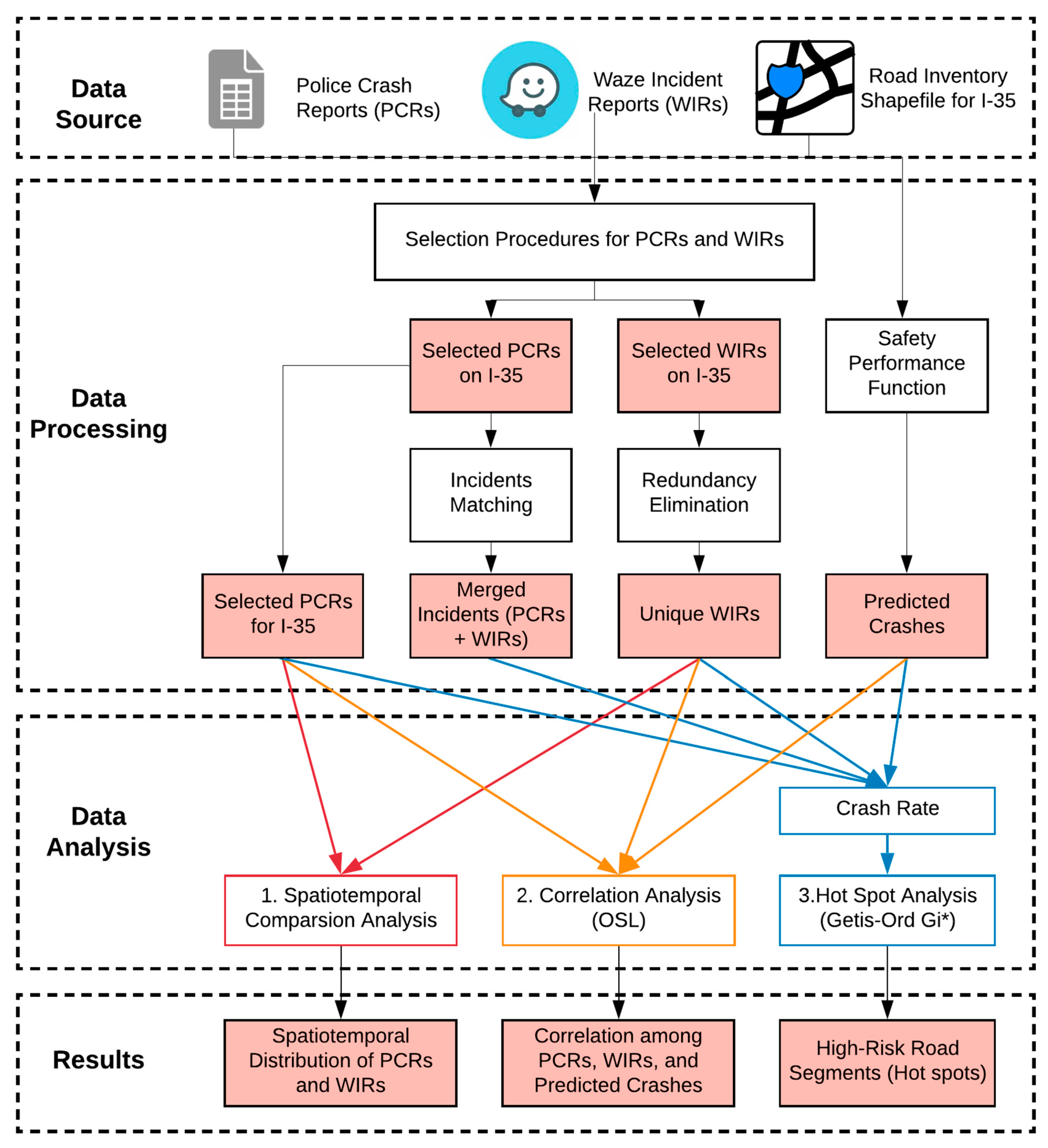
Figure 1 illustrates the flow chart of the research methodology used in this paper. The researchers utilized three data sources, including PCRs, WIRs, and roadway inventory shapefiles. The researchers first selected freeway crashes from PCRs and WIRs by removing frontage road, ramp exit, and ramp entrance crashes. Then, the duplicate WIRs were eliminated to identify unique Waze incident events (unique WIRs). A similar process was performed to match the unique WIRs with PCRs to create a merged dataset (PCRs + WIRs). Meanwhile, the researchers calculated the predicted crash frequency using freeway safety performance functions (SPFs) and CMFs. Finally, the researchers created four safety datasets: WIRs, PCRs, merged dataset, and predicted crashes.

To better explore the potential of WIRs in road safety analysis, three analyses were conducted, including:

• Spatiotemporal comparison analysis: characterize the spatiotemporal distributions of PCRs and WIRs.
• Correlation analysis: investigate the relationship between PCRs, WIRs, and predicted crashes to test further if WIRs could be used as a surrogate safety measure when PCRs are unavailable.
• Hot spot analysis:

  (1)

  calculate crash rates for each road segment using PCRs, unique WIRs, merged dataset, and predicted crashes, respectively;

  (2)

  perform hot spot analysis (Getis-Ord Gi *) using different crash rates to identify high-risk road segments. This analysis aims to evaluate if WIRs could capture more traffic risks ignored by the conventional crash datasets (e.g., PCRs).

3.1. Data Overview

This section explores the data sources and elements used in this paper.

3.1.1. Waze Incidents Reports (WIRs) Acquisition and Selection

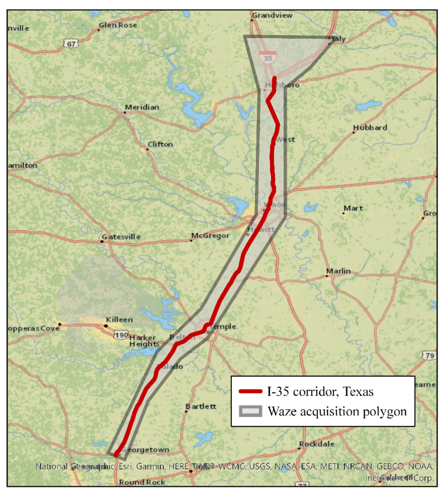
In 2014, Waze launched a two-way data exchange program—Connected Citizens Program (CCP). Program partners can receive real-time user-reported traffic data from a customized polygon (Figure 2) through the CCP data portal. Waze formats the crowdsourced data as an XML/JSON file. Each data file has a “traffic alerts” section, which contains user-reported traffic events. Four main types of traffic events are specified, including accident, jam, weather hazard, and road closure. In this study, WIRs refer to the Waze traffic accident alerts.

Waze generates a reliability score (0–10) for each reported traffic alert to indicate how reliable the report is. Because the current CCP does not support historical Waze data retrieval, the researchers carefully selected four weeks’ Waze data files from a 109 miles-long corridor on Interstate 35 (I-35) in North Texas (Figure 2); 2767 WIRs were collected from four weeks during August, October, November, December of 2016—one full week for each month, no holidays within the selected weeks. To extract the highly reliable WIRs, a selection procedure was implemented to filter out the unrelated and unreliable WIRs based on two criteria:

• Criteria 1: reliability score > 5 AND street name = I-35
• Criteria 2: reliability score > 5 AND road type = Freeways AND distance to I-35 < 60 m (~200 feet).

If a WIR could satisfy any criteria, it would be counted as a reliable WIR. Through this procedure, 1807 highly reliable WIRs were selected and then mapped to the nearest road segments identified from the roadway inventory shapefiles.

3.1.2. Police Crash Reports (PCRs) Acquisition and Selection

PCRs were collected from the Texas Department of Transportation (TxDOT) Crash Records Information System (CRIS) [16]. Data for crashes deemed “TxDOT reportable” are characterized as the crash which occurs on a public roadway and results in a fatality, injury, or a minimum of $1000 in damage. It contains information collected in Texas Peace Officer’s Crash Report (CR-3), interpreted data based on CR-3 information, system-generated data based on CR-3 information, and roadway attribute data from Texas Inventory.

First, the researchers selected the crashes, which were reported during the same period of WIRs and within 60 m (~200 ft) of I-35. This buffer was selected based on the roadbed width of the freeway. A selection procedure was then applied based on the attributes of PCRs to eliminate unrelated crash reports (e.g., frontage road or ramp crashes). After filtering, 177 freeway crashes were identified, which occurred in the study site during the four-week study period:

• Criteria: roadway part (on which crash occurred) = main/proper lane AND roadway system = Interstate AND whether a crash occurred at an intersection and ramp = No.

3.1.3. Roadway Characteristics

The researchers obtained roadway design elements and traffic volumes (annual average daily traffic (AADT)) from TxDOT’s Roadway Inventory shapefiles [17]. The corridor stretches for 109.956 miles and consists of 294 segments. Descriptive statistics of roadway characteristics are detailed in

Table 2. Descriptive statistics of road inventory data in the study site.

Roadway Design Elements	Maximum	Minimum	Mean	Std. Dev.
Length (in miles)	4.136	0.001	0.374	0.530
Annual average daily traffic (AADT)	132,225	56,176	73,685.068	14,747.346
Lane Width (in feet)	20	11	12.238	1.135
Inside Shoulder Width (in feet)	32	0	13.745	5.699
Outside Shoulder Width (in feet)	44	0	20.065	4.460
% of Trucks in AADT	30.3	1.2	25.260	4.089
Median Width (in feet)	50	3	28.432	9.076
Typical Segment Types (Number of Segments)	82	Urban 6-lane	Urban 4-lane	58
	108	Rural 6-lane	Rural 4-lane	46

.

3.2. Data Processing and Integration

This section explores the data processing and integration methods used in this paper.

3.2.1. WIRs Redundancy Elimination and Matching with PCRs

Since Waze users voluntarily contribute WIRs, different users may report the same incident, which generates a massive volume of redundant WIRs. Meanwhile, studies have proven that Waze can report on crashes from 20 min earlier to several hours later than PCRs with up to several miles positioning difference [12]. Following the recommended matching thresholds in Amin-Naseri et al. [12]—2.5-mile radius (spatial unit) and two hours of time lag (temporal unit)—the researchers tested different combinations of spatial and temporal thresholds for merging duplicate WIRs and matching them with PCRs:

• Spatial threshold range: from 0–3500 m (~2.5 miles) with 250 m (~0.15 miles) increment
• Temporal threshold range: from −20 (minutes earlier than PCRs)–120 (minutes later than PCRs) with a 10-min increment

The researchers hypothesize that the number of matched WIRs should experience a significant increase when the increasing thresholds reach their optimal values. Hence, a t-test was adopted to identify the significant increase to aid in determining the optimal thresholds. Please note that all the WIRs and PCRs were pre-processed through the selection procedure, as mentioned above, to make sure they report on the traffic information that had occurred on I-35 during the selected study period.

Unique WIRs: The duplicate WIRs can be further identified and grouped using the selected spatial and temporal thresholds, which refers to different traffic incidents. To merge the duplicate WIRs, the researchers proposed a weighting method to recalculate the location of each unique traffic incident based on the geolocations and reliability scores of the duplicate WIRs using Equations (1) and (2), as shown below:

$$x=\frac{{\sum }_{i=1}^n{x}_i{w}_i}{{\sum }_{i=1}^n{w}_i},$$

(1a)

$$y=\frac{{\sum }_{i=1}^n{y}_i{w}_i}{{\sum }_{i=1}^n{w}_i},$$

(1b)

where $x, y$ are the recalculated latitude and longitude of the unique incident, $i$ is the i-th duplicate WIRs, $n$ is the number of duplicate WIRs reporting on the same incident, $w_i$ is the weight signed to the i-th WIR using Equation (2), which depends on the generated reliability score for the i-th WIR ($r_i$):

$$w_i=\frac{r_i}{{\sum }_{i=1}^n{r}_i}$$

(2)

Merged Dataset: After generating the unique WIRs, the same thresholds were utilized to match WIRs with PCRs. The matched WIRs were treated as redundant reports and removed. The rest of the WIRs were combined with PCRs to form a new merged dataset, which covers both officially reported crashes and crowdsourced traffic incidents.

3.2.2. Predictive Models for Crash Frequency Estimation

To better evaluate the ability of WIRs for representing traffic risks, this study also compared WIRs with the predicted crashes calculated through the Highway Safety Manual’s (HSM) predictive methods [18]. According to this method, the predicted crashes are calculated as Equation (3):

$$N_{predicted}= N_{SP{F}_x}\times \left(CM{F}_{1x}\times CM{F}_{2x}\times \cdots CM{F}_{nx}\right)\times C_x$$

(3)

where $N_{predicted}$ is the predicted crash frequency for a study site $x$, $N_{SP{F}_x}$ is the predicted crash frequency based on a given base condition using SPF for study site $x$, $CM{F}_{nx}$ is the n-th CMF, and $C_x$ is the calibration factor for the jurisdiction of the study site $x$.

In this study, the researchers used four SPFs developed by Bonnesson and Pratt [19] to estimate the base condition highway crashes on four facility types in Texas: urban four-lane freeways, rural four-lane freeways, urban six-lane freeways, and rural six-lane freeways. The researchers then used five CMFs to estimate the predicted crashes: lane width, outside shoulder width, inside shoulder width, median width (no barrier), and truck presence. Refer to [19] for a detailed explanation of how to calculate SPFs and CMFs. As mentioned above, this study focuses on freeway crashes. Therefore, all the frontage and ramp entrance and exit SPFs and CMFs were excluded.

3.3. Data Analysis Methods

This study conducted three types of data analyses to evaluate the performance of using WIRs in the highway safety analysis. The researchers first performed spatiotemporal comparison analysis between PCRs and unique WIRs to assess the coverage of WIRs. The researchers then investigated the relationship between PCRs, unique WIRs, and predicted crashes to explore further if WIRs could be used as a surrogate data source when PCRs are unavailable. Last, high-risk road segments were identified by performing hot spot analysis (Getis-Ord Gi *) on the crash rates of road segments. In this study, four crash rates were calculated for each road segment based on different data sources, including PCRs, unique WIRs, merged dataset, and predicted crashes.

3.3.1. Crash Rate Calculation

Crash risk is commonly defined as “the number of crashes compared to the level of exposure,” which can better represent the likelihood of crash occurrence for a road segment [20]. In this study, the crash rate was calculated to indicate the “Risk-Level” of road segments. Equation (4) was adapted from [20] with:

$$R=\frac{C\times \mathrm{100,000,000}}{T\times V\times L}$$

(4)

where $R$ represents the crash rate of a road segment defined as “crashes per 100 million vehicle-miles of driving”; $C$ is the number of crashes occurred along a road segment; $T$ depicts time span (number of days); $V$ is Average Annual Daily Traffic (AADT) volumes; L is road segment length in miles.

In this study, four data sources, including PCRs, unique WIRs, WIR-PCR, and predicted crashes, were used to calculate different crash rates for each road segment.

3.3.2. Hot Spot Analysis (Getis-Ord Gi *)

The Getis-Ord Gi* statistic has been widely adopted to identify the significant spatial clusters of high values (hot spots) and low values (cold spots) [21,22]. It examines each sample within the context of its neighboring samples. The Gi * statistic is calculated using Equations (5)–(7) [22]:

$$G_i^{*}=\frac{{\sum }_{j=1}^n{w}_{i,j}{x}_j-\overline{X}{\sum }_{j=1}^n{w}_{i,j}}{S\sqrt{\frac{\left[n{\sum }_{j=1}^n{w}_{i,j}^2-{\left({\sum }_{j=1}^n{w}_{i,j}\right)}^2\right]}{n-1}}},$$

(5)

where,

$$\overline{X}= \frac{{\sum }_{j=1}^n{x}_j}{n},$$

(6)

$$S= \sqrt{\frac{{\sum }_{j=1}^n{x}_j^2}{n}-{\left(\overline{X}\right)}^2}$$

(7)

$n$ represents the number of samples, $x_j$ is the value of j-th sample, and $w_{i,j}$ indicates the spatial weight between two samples$\left(i, j\right)$.

Gi * statistic generates a z-score and p-value for each feature. The statistically significant positive z-scores indicate hot spots—clusters of high values; the negative z-scores refers to cold spots—clusters of low values. In this study, Gi * statistic was performed to identify hot spots of high-risk road segments—statistically significant clusters of high crash rates. By comparing the hot spots generated from different data sources, the researchers could further examine whether the WIRs could better represent traffic risks.

4. Results

This section covers the redundancy elimination result of WIRs, the merged dataset by matching WIRs with PCRs. It also details the results of three analyses, including spatiotemporal comparison analysis, correlation analysis, and hot spot analysis.

4.1. Result for WIRs Redundancy Elimination and Matching with PCRs

The researcher used the “true” incident, i.e., the PCR, as the starting point and tested different combinations of spatial and temporal thresholds to (a) remove the redundant WIRs that correspond to the same PCR; and (b) match unique WIRs with the PCRs. The researchers hypothesize that when spatial and temporal “distances” from the true incident (i.e., PCR) to the surrogate incident (i.e., WIR) reach their optimal value, the number of matched WIRs should experience a significant increase since more redundant WIRs can be captured. After the optimal threshold is attained, the number of matched WIRs should not be significantly different than the optimal number of matched WIRs.

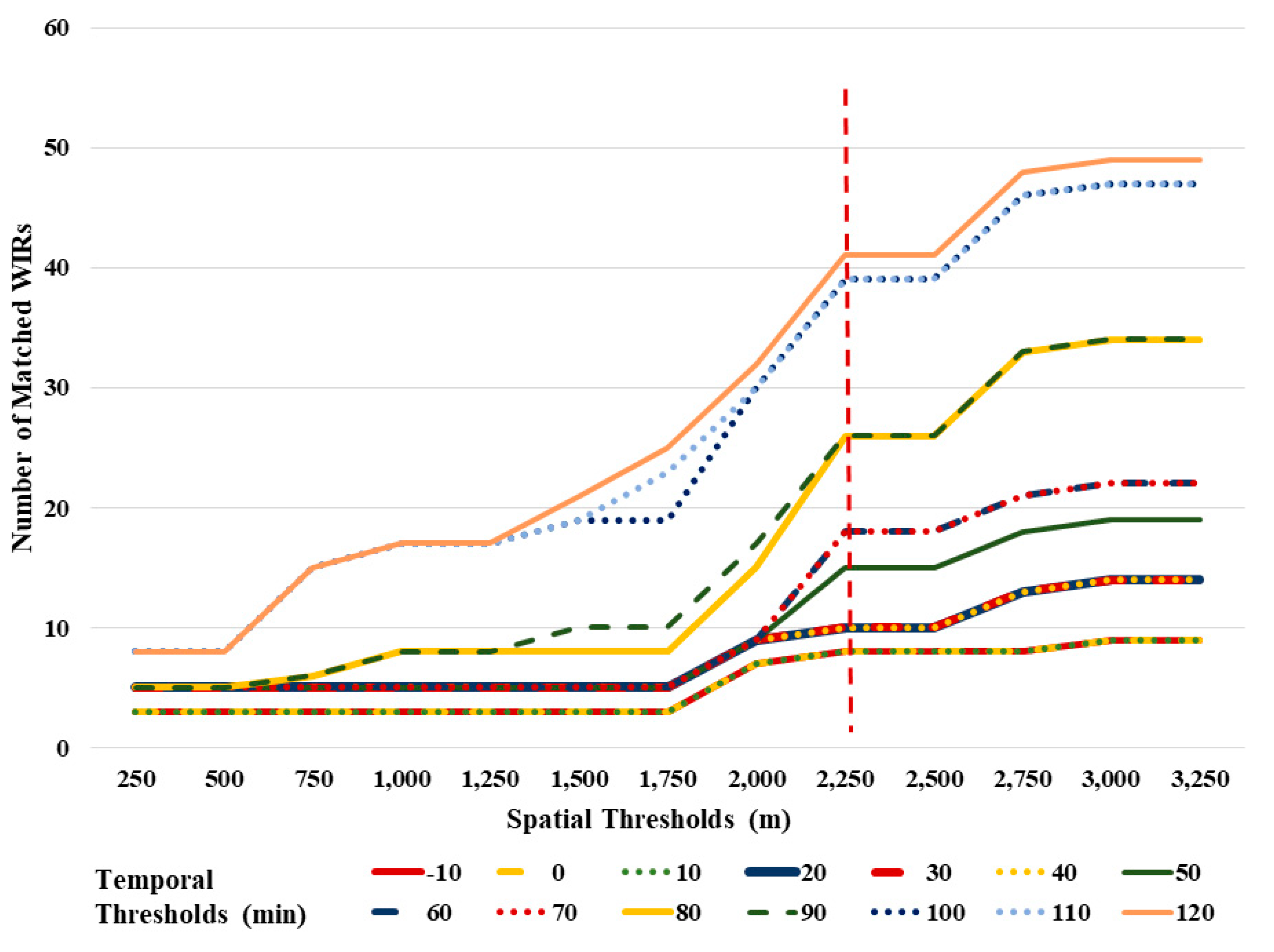
Figure 3 illustrates the number of WIRs matched with PCRs when using each combination of spatial and temporal thresholds. As can be observed, regardless of the time interval, the number of unique WIRs increases consistently until the distance from the true incident (i.e., PCR) reaches 2250 m (~1.4 miles). After this distance, the number of WIRs matched with the PCR become steady. A new jump is observed at 2500 m, although it does not seem to be very significant. It is possible that this “second” jump in the number of unique WIRs matching with the PCR refers to a secondary event that was related to the primary event. However, this hypothesis cannot be verified because, as indicated earlier, near-crashes and traffic incidents are not reported by police. Hence, the researchers selected the 2250 (or 1.4 miles) as the spatial threshold for identifying the redundant WIRs.

To determine the best temporal threshold, the researchers used a t-test to check the significant difference in the number of matched WIRs for different time intervals. A t-test is a widely utilized statistical test to compare two data groups, which can determine if they are statistically different. Studies have found that Waze can report a crash from 20 min earlier to several hours later than the police-reported crash time [12]. Therefore, the researchers tested different temporal intervals to match WIRs with PCRs. These temporal intervals have the same start-timestamp (−20 min earlier than PCRs) and a different end-timestamp. The temporal thresholds $t$ in Figure 3 represent the end-timestamps for each temporal matching interval. For example, $t=10$ represents a 30-min temporal matching interval—from 20 min earlier to 10 min later than PCR occurred. The researchers tested different temporal thresholds ranging from −10 min (i.e., 10 min earlier than PCRs) to 120 min (i.e., two hours after the PCR) in 10-min increments.

Figure 3 shows that the number of WIRs matched with a PCR remains the same when the temporal threshold increases from −10 to 10; hence, they are used as a baseline dataset (BD) to compare to the number of matched WIRs reported at higher time intervals. This dataset is denoted as BD = [$N_{WIR,-10},N_{WIR,0},N_{WIR,10}$], where $N_{WIR,t}$ refers to the number of WIRs matched with the PCR with a temporal matching interval, $t=-10$ (from 20 min earlier to ten minutes earlier), $t=0$ (from the 20 min earlier to the same time as the PCR) and $t=10$ (from the 20 min earlier to 10 min later than the PCR). The comparison datasets (CD_r) were then generated by adding 10-min intervals to the baseline dataset and compared with BD using a t-test to identify the significant difference between the number of baseline and comparison WIRs. For example, CD₃₀ refers to: [$N_{WIR,-10},N_{WIR,0},N_{WIR,10}, N_{WIR,20}, N_{WIR,30}$]).

Table 3. t-test results between base dataset and comparison datasets.

Goodness of Fit Statistics	CD20	CD30	CD40	CD50	CD60	CD70
t-statistic	−1	−1.63299	−2.23607	−1.98248	−2.2088	−2.6295
p-value one-tail	0.195501	0.088904	0.037793	0.047349	0.031454	0.015101
t Critical one-tail	2.353363	2.131847	2.015048	1.94318	1.894579	1.859548
p-value two-tail	0.391002	0.177808	0.075587	0.094698	0.062909	0.030201
t Critical two-tail	3.182446	2.776445	2.570582	2.446912	2.364624	2.306004

summarizes the results of the t-test, including t-statistic (aka t-value), the p-value for one- and two-tailed tests, and the t Critical value for one- and two-tailed tests. Among these statistics, the p-value is the most important to determine whether two groups are statistically different. In general, we use a two-tailed t-test to evaluate the difference between two groups and use a one-tailed t-test to assess if one group’s mean value is higher or lower than the other group. Therefore, to identify if a significant difference exists between BD and CDr, we checked the p-value of two-tailed t-tests. The result shows that the t-test between BD and CD70 yields a statistically significant p-value (<0.05). It indicates, when choosing 70-min as the end-timestamp, the number of matched WIRs was observed to be significantly different than the previous results, implying that the temporal threshold for matching WIRS and PCRs should be 90 min (from the 20 min before to 70 min later than the PCR).

As the results of these analyses, the researchers determined the optimal spatial and temporal thresholds for identifying the redundant WIRs as:

• Spatial threshold: in a 2250-m radius.
• Temporal thresholds: 90 min (−20 to 70 min).

By applying these thresholds, 1807 WIRs were finally consolidated into 381 unique WIRs. The location for each unique WIRs was recalculated using the proposed weighting method (Equations (1) and (2)).

A similar process was conducted to match unique WIRs with PCRs. In this study, only 13 out of 177 PCRs (7.34%) were matched with the unique WIRs (13 out of 381). These results align with prior studies showing that 7 to 13.4 percent of reported crashes can be matched with the Waze reports [12,13].

Finally, the researchers created a merged database by combining PCRs with un-matched unique WIRs. This dataset contains 545 traffic incidents and crashes.

4.2. Spatiotemporal Comparison Analysis

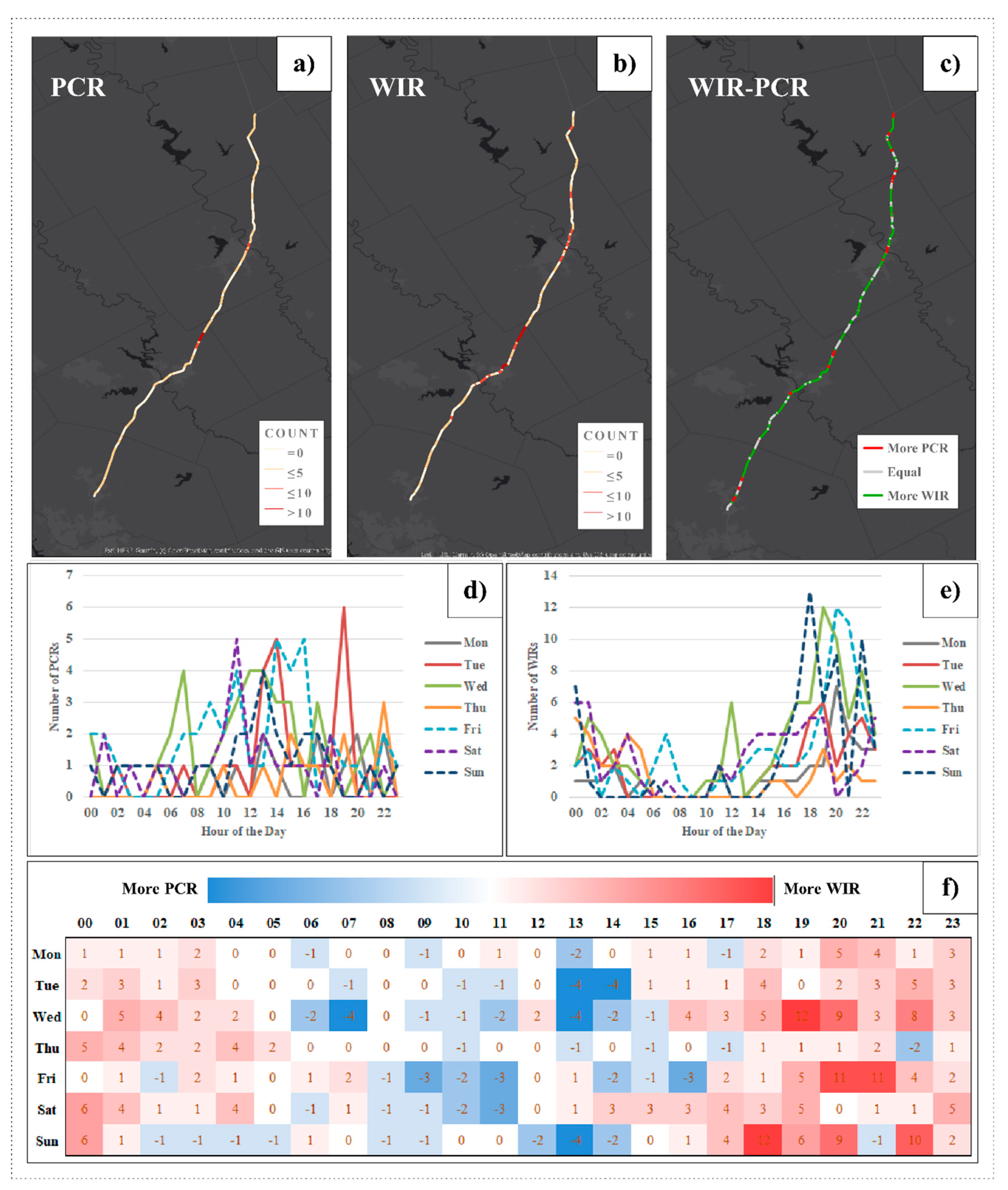
The spatiotemporal distribution of PCRs and unique WIRs are plotted in Figure 4. Figure 4a,b represent the counts of PCRs and unique WIRs for each road segment. These two figures show a similar spatial data pattern, which implies that crash-intense road segments can potentially be captured using WIRs. Figure 4c shows the differences between PCRs and WIRs. Among 109.96 miles of roadway segments in this study, 66.24 miles of road segments experienced more WIRs than PCRs, which means that WIRs have broader spatial coverage than PCRs.

The temporal distribution of WIRs and PCRs are depicted in Figure 4d,e. These figures show that PCRs tend to occur during the daytime, while WIRs were more intensively reported at nighttime. However, the previous studies state that Waze is less reported during the midnight period, which conflicts with the researchers’ finding (11). This finding implies that the temporal pattern of WIRs may vary in different study areas.

Figure 4f shows the hourly comparison result, which indicates that more PCRs are recorded than WIRs from 8:00 to 14:00. From 18:00 to 5:00, more Waze reports incidents observed than officially reported crashes.

4.3. Correlation Analysis

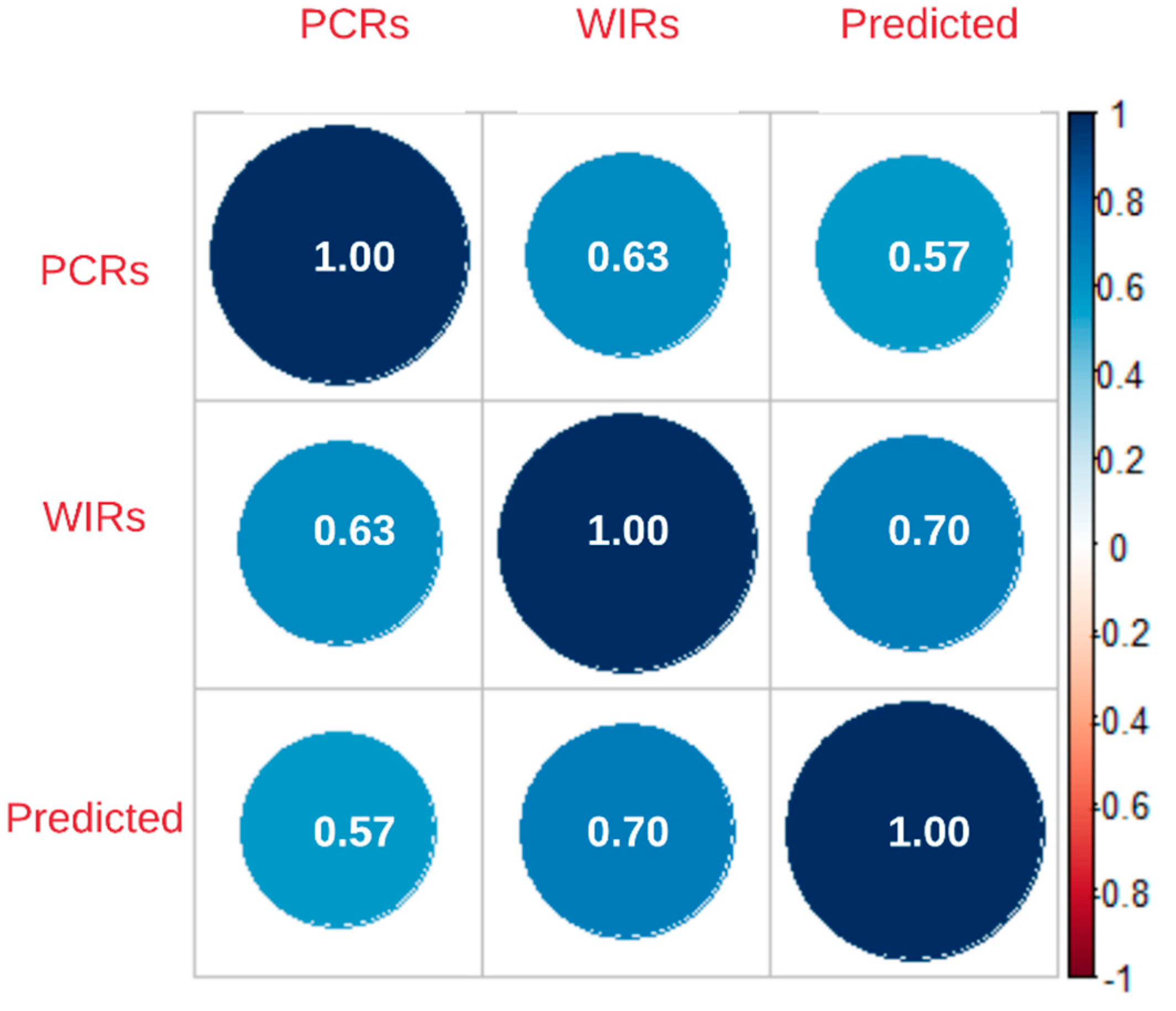
This study investigated the relationship between PCRs, unique WIRs, and the estimated crashes through predictive models to statistically test if WIRs could be used as a surrogate data source or safety measures in the absence of crash data. The correlation between these three datasets is detailed in Figure 5. This figure illustrates that PCRs are highly correlated with WIRs (0.63) than with predicted crashes (0.57). It also suggests that WIRs can better represent the predicted safety risk than PCRs (0.70 vs. 0.57).

The researchers also developed the Ordinary Least Square (OLS) regression model to investigate the relationship between the three safety measures: PCR, WIR, and predicted crashes. Two regression models were constructed. One uses unique WIRs alone as an independent variable (Equation (8)); another uses both WIRs and predicted crashes as independent variables (Equation (9)). The estimation results are shown in

Table 4. Linear regression results for PCRs.

Model Parameters	Model 1	Model 2
	Estimate (St. D.)	Estimate (St. D.)
Intercept	0.144 (0.069)	0.030 (0.072)
Unique WIRs	0.354 *** (0.025)	0.255 *** (0.035)
Predicted Crashes		0.123 *** (0.031)
R-squared	0.402	0.434
Adjusted R-squared	0.400	0.430
No. observations	294

Standard errors are included in parenthesis. *** represents significance at 99% level based on p-value.

and have the following functional forms:

$$N_{PCR}=0.144+0.354\times N_{WIR}$$

(8)

$$N_{PCR}=0.030+0.255\times N_{WIR}+0.123\times N_{Predicted}$$

(9)

where $N_{PCR}$ is the calculated number of PCRs for a road segment, $N_{WIR}$ is the number of unique WIRs, and $N_{Predicted}$ is the predicted number of crashes using SPFs and CMFs.

The regression results indicate that the number of unique WIRs is a significant predictor for estimating crashes reported on each road segment. When taking both unique WIRs and predicted crashes as predictors, the model’s performance can be slightly improved with R-squared increased from 0.4 to 0.43.

4.4. Hot Spot Analysis

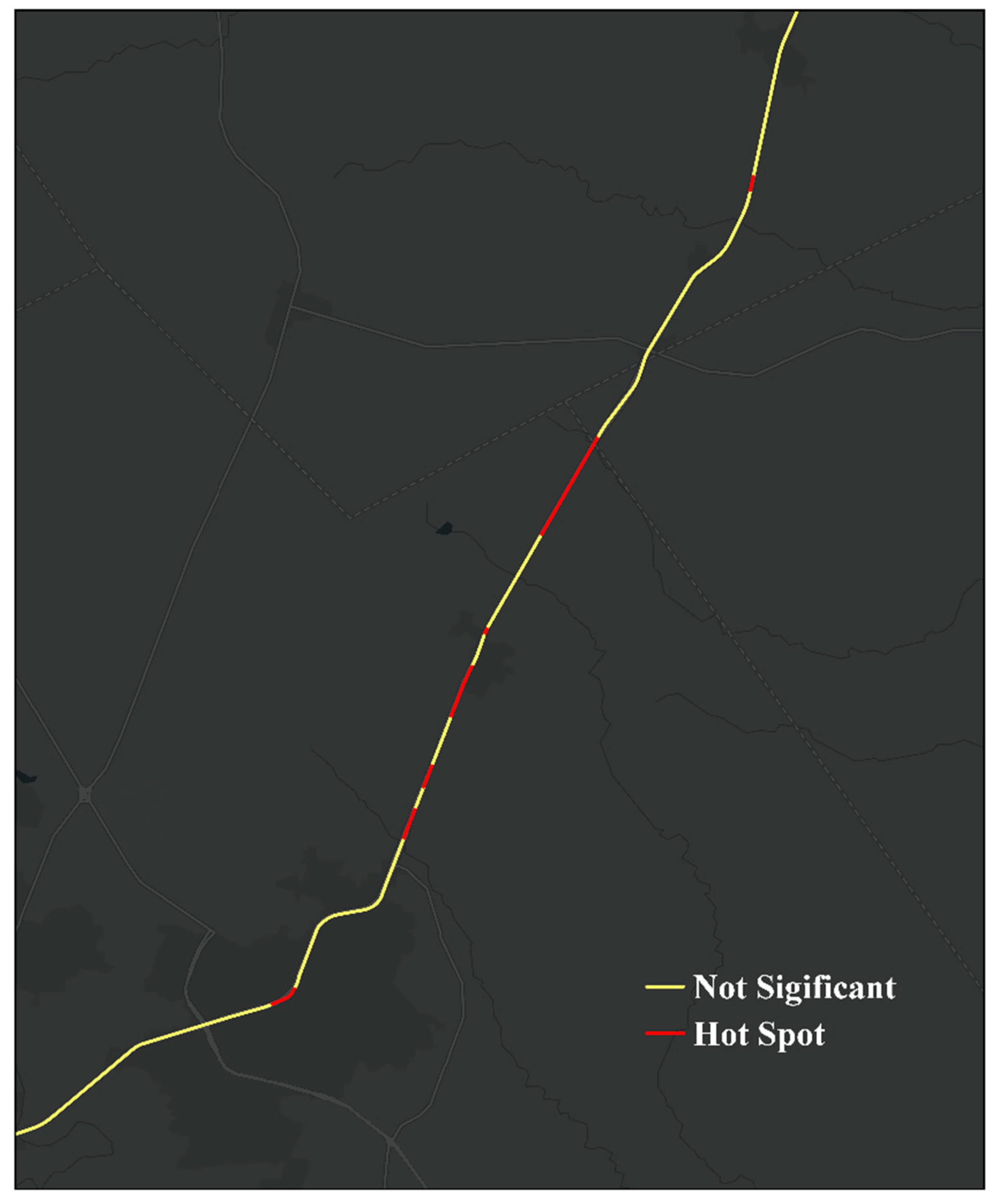
This study also assessed the performance of WIRs for identifying high-risk road segments. The researchers first calculated crash rates for each road segment using four different data sources, including PCRs, unique WIRs, merged dataset, and predicted crashes. Then, Getis-Ord Gi * statistics were conducted based on different crash rates to identify hot spots—high-valued road segments surrounded by high-valued neighboring segments. Figure 6 illustrates the sample result of detected hot spots, which were generated using one-week unique WIRs collected from December 2016. To maximally capture potential risky locations, segments with a confidence level above 90 percent were identified as hot spots, visualized as red lines in Figure 6.

This study compared hot spots detected from different data sources in different months to investigate if hot spots vary from month to month. The researchers also examined the monthly results with the hot spots detected from four-month datasets to identify constant hot spots. This study defines constant hot spots as a segment or its neighboring segments (within ± 1 mile) that (1) are determined as hot spots in more than two different months, and (2) also need to be identified as hot spots in the four-month dataset.

Table 5. Hotspot detection and comparison results.

Datasets	August	October	November	December	Four-month
PCRs	266, 278, 318, 323, 334, 337, 341, 350, 352, 354, 355, 357, 363	266, 276, 298, 299, 303, 306, 308, 310, 317, 327, 351, 356, 358, 368	291, 292, 303, 306, 308, 318, 333, 334, 343, 351, 353, 358, 363, 367	266, 288, 303, 306, 317, 332, 334, 342	266, 298, 303, 317, 334, 342, 358, 363
WIRs	294, 318, 319, 356, 363, 364	298, 299, 303, 305, 307, 308, 310, 315, 319, 344, 350, 356, 357, 366, 368	291, 303, 315, 318, 336, 344, 357, 363, 368	291, 299, 303, 305, 306, 308, 310, 318, 327, 332, 350, 359	284, 294, 303, 307, 315, 317, 319, 344, 356, 357, 363, 364, 368
Merged dataset (WIR+PCR)	264, 266, 294, 318, 319, 337, 352, 354, 355, 356, 363, 364, 366, 367	248, 298, 299, 303, 307, 308, 310, 315, 317, 319, 336, 351, 356, 357, 358, 366, 368	291, 292, 303, 315, 317, 318, 334, 344, 358, 363, 368	266, 291, 305, 308, 327, 332, 342, 334, 350, 359,	284, 294, 298, 303, 315, 317, 334, 336, 356, 357, 358, 363, 364, 368
Predicted Crashes (2016)	317, 363, 293, 317, 385
Numbers represent distance from origins (DFOs) for road segments. Underscore represents constant hot spots. Bold text indicates hot spots matched with merged dataset hot spots.

details the results of hotspot detection using PCR, WIR, merged dataset, and predicted crashes. The numbers listed in this table represent the integer part of distance from origin (DFO) for the detected high-risk road segments, making it easier to locate the identified hot spots. If any portion of a one-mile-segment was recognized as a hot spot in this study, the researchers would count the entire one-mile-segment as a high-risk road segment. Constant hot spots are highlighted with underscores. The matched segments are marked with bold text.

This table shows that the hot spots may vary in different months; however, there are still some constant hot spots that may be considered true high-risk segments. By combing PCRs with WIRs (merged dataset), 14 segments (refer to 14 miles) were identified as hot spots from the four-month dataset, which is longer than the segments identified from PCRs (8 miles), WIRs (13 miles), and predicted crashes (5 miles). By comparing the hot spots detected from different datasets, we can notice that most of hot spots detected from PCRs (6/8 = 75%), WIRs (10/13 = 77%), and predicted crashes (5/5 = 100%) could be matched with the results of the merged dataset. It implies that combining PCRs and WIRs can capture more potentially risky sites.

5. Discussion

As an emerging data source, Waze shows excellent potential to capture a broad range of unreported traffic incidents. However, current Waze-related studies are still at a preliminary stage. How to better leverage Waze into road safety analysis is still an unanswered research question. This study provides new findings helping to answer the following three essential but underexplored Waze-related research questions.

Question 1: What are the spatiotemporal distribution characteristics of WIRs and PCRs?

Through the spatiotemporal comparison of PCRs and WIRs, the researchers found these two data sources show a very similar spatial distribution. However, the temporal comparison shows a significant difference between them. In this study, PCRs were reported during the daytime, while WIRs were more intensively reported during nighttime. It is also worth noting that 60.24 percent of the road segments in the study site received more WIRs than PCRs; 27.1 percent received the same amount of WIRs and PCRs. It implies that unreported traffic incidents more intensively occurred on most of the road segments. These traffic incidents should be considered in road safety studies.

Question 2: Can WIRs be used as a surrogate data source when PCRs are unavailable?

By matching WIRs with PCRs, the researchers found that only 7.34 percent of the PCRs can be paired with WIRs, which aligns with prior studies—13.4 percent [12] and 7 percent [13]. Therefore, it can be concluded that WIRs and PCRs report on different traffic risks. Correlation analysis shows that PCRs are highly correlated with WIRs (0.63) than with predicted crashes (0.57). It also indicates that WIRs can better represent the predicted traffic risk than PCRs (0.70 vs. 0.57). The regression models suggest that both WIRs and predicted crashes are significant predictors for estimating PCRs. However, using WIRs alone may not be capable enough since the model performance is relatively unsatisfying with an R-squared of 0.4. Meanwhile, the similar spatial distributions of WIRs and PRCs suggest that Waze data might be able to identify crash-intense road segments when PCRs are unavailable. This finding has very significant implications for highway safety researchers and practitioners. It indicates that WIRs have the potential to be used as surrogate safety measure in the absence of crash data (e.g., when evaluating the safety effectiveness of new safety treatments). However, further research is required in order to confirm this finding.

Question 3: Can the crash hot spots be better captured by integrating WIRs and PCRs?

By comparing the hot spots generated from different months, the researchers found the detected high-risk road segments may vary in different months. However, it is worth noting that some hot spots can be persistent in different months, which are constant high-risk segments and should be given more attention. This study has found that, by combining WIRs with PCRs, more high-risk road segments can be identified (14 miles) comparing to the results generated from PCRs (8 miles), unique WIRs (13 miles), and predicted crashes (5 miles). Most of the hot spots detected from PCRs (75%), unique WIRs (77%), and predicted crashes (100%) could be identified from the merged data. Therefore, it can be concluded that integrating WIRs and PCRs can better capture traffic risks and discover more unidentified high-risk road segments.

6. Conclusions

This study is among the first to systemically evaluate Waze incident reports (WIRs) for capturing unreported near-crashes and traffic incidents. The researchers first proposed a new procedure to eliminate duplicate WIRs to extract unique WIRs. Meanwhile, these unique WIRs were further matched with police crash reports (PCRs) to form a new merged dataset, which covers both officially reported crashes and crowdsourced incidents. This study also calculated the crash frequency of road segments based on the road inventory shapefile using the HSM predictive methods. Three analyses were conducted to assess the effectiveness of WIRs in road safety analysis comprehensively. The main findings are summarized as follows:

• PCRs and WIRs show a very similar spatial distribution; however, their temporal distribution can be significantly different.
• PCRs are highly correlated with WIRs, suggesting that WIRs can be a strong predictor in crash prediction models.
• By combining PCRs and WIRs, more high-risk road segments can be identified, which suggests that both official crash records and crowdsourced traffic incidents need to be considered in future safety analysis.

However, there are still some gaps that were not adequately addressed in this study. Although the findings are promising, the researchers used Waze data only from an interstate corridor, which is generally assumed to experience more Waze reports. This gap may also affect some of the findings; for example, the temporal and spatial threshold for consolidating the WIRs and matching them with PCRs may not be applicable to other facility types. Meanwhile, new strategies for integrating crowdsourced incidents with observed crashes into safety hotspot analysis need to be further explored (e.g., assigning different weights to incidents and crashes). Future research will focus on these areas.

References

- World Health Organization Global Status Report on Road Safety. 2018. Available online: https://www.who.int/violence_injury_prevention/road_safety_status/2018/en/ (accessed on 28 January 2019).
- U.S. National Highway Traffic Safety Administration Traffic Safety Facts 2016 Data. Available online: https://crashstats.nhtsa.dot.gov/Api/Public/ViewPublication/812580 (accessed on 25 August 2019).
- Li, X.; Goldberg, D.W. Toward a mobile crowdsensing system for road surface assessment. Comput. Environ. Urb. Syst. 2018, 69, 51–62. [Google Scholar] [CrossRef]
- Fire, M.; Kagan, D.; Puzis, R.; Rokach, L.; Elovici, Y. Data Mining Opportunities in Geosocial Networks for Improving Road Safety. In Proceedings of the 2012 IEEE 27th Convention of Electrical and Electronics Engineers in Israel, Eilat, Israel, 14–17 November 2012. [Google Scholar]
- Silva, T.H.; Vaz De Melo, P.O.S.; Viana, A.C.; Almeida, J.M.; Salles, J.; Loureiro, A.A.F. Traffic condition is more than colored lines on a map: Characterization of Waze alerts. In Lecture Notes in Computer Science (Including Subseries Lecture Notes in Artificial Intelligence and Lecture Notes in Bioinformatics); Springer: Cham, Switzerland, 2013; Volume 8238, pp. 309–318. [Google Scholar]
- Li, X.; Huo, D.; Goldberg, D.W.; Chu, T.; Yin, Z.; Hammond, T. Embracing crowdsensing: An enhanced mobile sensing solution for road anomaly detection. ISPRS Int. J. Geo. Inf. 2019, 8, 412. [Google Scholar] [CrossRef] [Green Version]
- Waze Waze Company Factsheet. Available online: https://assets.brandfolder.com/p31v19-dpmnts-ci9it3/original/WazeCompanyFactsheet.pdf (accessed on 18 July 2019).
- Monge-Fallas, J.; Hernandez-Castro, F.; Gonzalez-Villalobos, S.; Barquero-Rodriguez, E.; Esquivel-Piedra, J. Traffic Data Visualization in costa Rica: A Visualization of Top 100 Routes with the Highest Traffic Density in Costa Rica. PONTE Int. Sci. Res. J. 2016, 72, 262–273. [Google Scholar] [CrossRef]
- Perez, G.V.A.; Lopez, J.C.; Cabello, A.L.R.; Grajales, E.B.; Espinosa, A.P.; Fabian, J.L.Q. Road Traffic Accidents Analysis in Mexico City through Crowdsourcing Data and Data Mining Techniques. Int. J. Comp. Inf. Eng. 2018, 12, 604–608. [Google Scholar]
- Estrada, S.R.F.; Molina, A.; Perez-Espinosa, A.; Reyes, C.A.L.; Quiroz, F.J.L.; Bravo, G.E. Zonification of Heavy Traffic in Mexico City. In Proceedings of the International Conference on Data Mining (DMIN), Las Vegas, NV, USA, 25–28 July 2016. [Google Scholar]
- Goodall, N.; Lee, E. Comparison of Waze crash and disabled vehicle records with video ground truth. Transp. Res. Interdiscip. Perspect. 2019, 1, 100019. [Google Scholar] [CrossRef]
- Amin-Naseri, M.; Chakraborty, P.; Sharma, A.; Gilbert, S.B.; Hong, M. Evaluating the Reliability, Coverage, and Added Value of Crowdsourced Traffic Incident Reports from Waze. Transp. Res. Rec. 2018, 2672, 34–43. [Google Scholar] [CrossRef] [Green Version]
- Dos Santos, S.R.; Davis, C.A.; Smarzaro, R. Integration of Data Sources on Traffic Accidents. In Proceedings of the Brazilian Symposium on GeoInformatics, Campos do Jordão, SP, Brazil, 27–30 November 2016; National Institute for Space Research, INPE: São José dos Campos, Brasil, 2016; Volume 2016, pp. 192–203. [Google Scholar]
- Flynn, D.; Gilmore, M.; Sudderth, E. Estimating Traffic Crash Counts Using Crowdsourced Data: Pilot Analysis of 2017 Waze Data and Police Accident Reports in Maryland; Volpe National Transportation Systems Center: Cambridge, MA, USA, 2018. [Google Scholar]
- Parnami, A.; Bavi, P.; Papanikolaou, D.; Akella, S.; Lee, M.; Krishnan, S. Deep Learning Based Urban Analytics Platform: Applications to Traffic Flow Modeling and Prediction. In ACM SIGKDD Workshop on Mining Urban Data (MUD3); ACM: London, UK, 2018. [Google Scholar]
- Texas DOT Crash Records Information System. Available online: https://cris.dot.state.tx.us/public/Purchase/app/home/welcome (accessed on 25 July 2019).
- Texas DOT Roadway Inventory. Available online: https://www.txdot.gov/inside-txdot/division/transportation-planning/roadway-inventory.html (accessed on 25 July 2019).
- American Association of State Highway and Transportation Officials. Highway Safety Manual, 1st ed.; American Association of State Highway and Transportation Officials: Washington, DC, USA, 2010. [Google Scholar]
- Bonneson, J.A.; Pratt, M.P. Roadway Safety Design Workbook.; Texas Transportation Institute: Bryan, TX, USA, 2009. [Google Scholar]
- The U.S. National Highway Safety Administration Crash Rate Calculations. Available online: https://safety.fhwa.dot.gov/local_rural/training/fhwasa1109/app_c.cfm (accessed on 5 July 2020).
- Songchitruksa, P.; Zeng, X. Getis-ord spatial statistics to identify hot spots by using incident management data. Transp. Res. Rec. 2010, 2165, 42–51. [Google Scholar] [CrossRef]
- Esri How Hot Spot Analysis (Getis-Ord Gi*) Works. Available online: https://pro.arcgis.com/en/pro-app/tool-reference/spatial-statistics/h-how-hot-spot-analysis-getis-ord-gi-spatial-stati.htm (accessed on 2 December 2020).
Figure 1.
Flow chart of research methodology.
Figure 2.
Study site and Waze reports acquisition polygon.
Figure 3.
Number of matched Waze incident reports (WIRs) when using different spatial and temporal thresholds.
Figure 4.
Spatiotemporal comparison between police crash reports (PCRs) and unique WIRs, including (a) spatial distribution of PCRs, (b) spatial distribution of unique WIRs, (c) spatial comparison between PCRs and unique WIRs, (d) hourly distribution of PCRs, (e) hourly distribution of unique WIRs, and (f) hourly comparison between PCRs and unique WIRs.
Figure 5.
Correlations among PCRs, unique WIRs, and predicted crashes.
Figure 6.
Sample result of detected hot spots.