Assessment of Rain Garden Effects for the Management of Urban Storm Runoff in Japan


1
School of Architecture, Nanjing Tech University, Nanjing 211800, China
2
Graduate School of Global Environmental Studies, Kyoto University, Yoshida-Honmachi, Sakyo-Ku, Kyoto 606-8501, Japan
3
Suzhou Erjian Construction Group Co., Ltd., Suzhou 215012, China
*
Author to whom correspondence should be addressed.
Sustainability 2020, 12(23), 9982; https://0-doi-org.brum.beds.ac.uk/10.3390/su12239982
Submission received: 22 September 2020
/
Revised: 25 November 2020
/
Accepted: 26 November 2020
/
Published: 29 November 2020
(This article belongs to the Section Sustainable Urban and Rural Development)
Abstract
:Storm runoff is a growing concern against a background of increasing urban densification, land-use adaptation and climate change. In this study, a storm water management model was used to analyze the hydrological and water-quality effects of rain gardens (also known as bioretention cells) as nonpoint source control solutions in low-impact development (LID) practices for an urban catchment in the Nakagyo Ward area of Kyoto in Japan. The results of simulations with input involving Chicago hyetographs derived for different rainfall return periods (referred to as 3 a, 5 a, 10 a, 30 a, 50 a and 100 a) indicated the effectiveness of this arrangement, in particular for rainstorm 3 a, which exhibited the maximum contaminant reduction ratio (Total Suspended Solids (TSS) 15.50%, Chemical Oxygen Demand (COD) 16.17%, Total Nitrogen (TN) 17.34%, Total Phosphorus (TP) 19.07%) and a total runoff reduction volume of 46.56 × 10⁶ L. With 5 a, the maximum number of flooding nodes was reduced to 87, demonstrating that rain gardens handle rainfall effectively over a five-year return period. There was a one-minute delay for 100 a, which again indicates that rain gardens support control of urban runoff and mitigate flooding. Such gardens were associated with reduced stormwater hazards and enhanced resistance to short-term rainstorms at the research site, and should be considered for urban planning in Kyoto and other cities all over the world.
1. Introduction
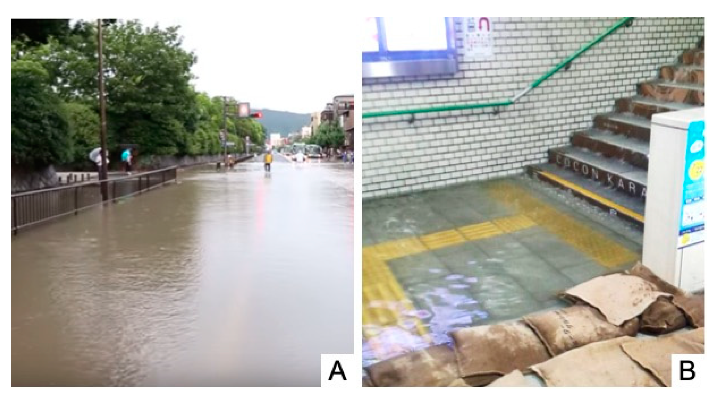
The ongoing replacement of urban green spaces with impervious surfaces creates a sharp decline in urban biodiversity [1,2], while creating issues with urban storm runoff associated with the increased intensity of rainfall volume/rate during the heavy rain and typhoons [3]. As runoff accelerates from these impervious surfaces, it carries more pollutants to water bodies and increases the loading of contaminants, which impact the water quality [4]. Against this background, a series of problems such as urban flooding and deterioration of water quality caused by urban storm runoff has become increasingly apparent worldwide [5,6,7,8]. As early as 2005, the average urbanization ratio in Japan was as high as 66% [9], with the urban land usage ratio (equals the land used for urban construction divide the total land area of the region) increasing significantly from 4.3% in 1976 to 7.3% in 2009 [10]. As a result of this elevated usage, the area of forests and farmland is gradually decreasing. Heavy rain on 16 August 2014 caused disastrous effects in the Nakagyo Ward area of Kyoto in Japan [11]. Shijo subway station was flooded, and the city’s central Marutamachi Street was submerged with storm runoff due to insufficient drainage capacity (Figure 1). Rapid urbanization, coupled with extreme weather, has caused frequent urban flooding in Japan, leading to significant property damage and numerous casualties [12,13,14,15].
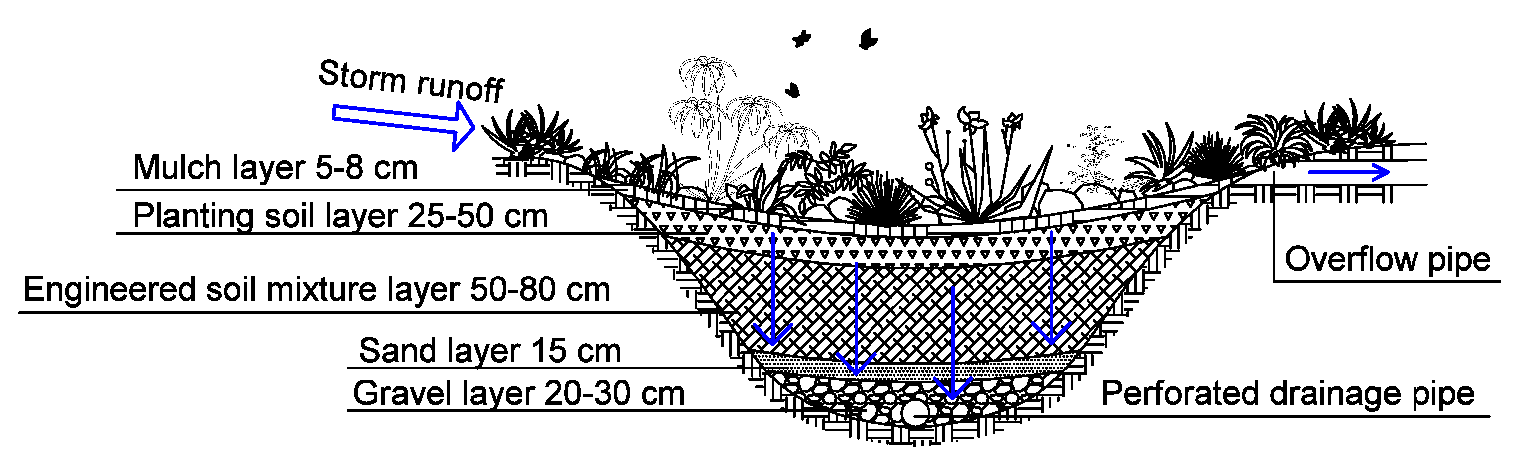
Rain gardens, also known as bioretention cells, consist of a depressed area with vegetations, engineered soil mixture and optional sand or gravel drainage bed, which meets the reuse water requirement. The engineered soil mixture includes different layers which are for the optimize infiltration and the growth of the plants [16,17,18,19]. Figure 2 shows the diagram of a typical rain garden structure. As runoff travels through the system, the vegetation acts as a buffer, which reduces the peak velocity and allows some suspended particles to settle down, promoting the removal of pollutants [20]. When the runoff enters the rain garden surface, it can be temporarily stored in a recessed space, which can relieve the pressure of urban drainage systems during heavy rains. Part of the water is filtered, stored and penetrated through the engineered soil mixture. The other amount of water promotes water purification through complex physical, chemical and biological processes between plants and soil. Part of the purified water flows into pre-buried perforated pipelines for recycling and reuse, while the other directly conserves groundwater. When the runoff exceeds the rain garden’s maximum output capacity, the excess water is discharged through the buried overflow pipe.
Reduction in runoff volume using rain garden systems is well documented [21,22,23,24,25], with a range of 23–97% (Table 1). A large number of studies have credited reducing 22–93% of water pollutant (Total Suspended Solids (TSS), Total Nitrogen (TN), Total Phosphorus (TP), Chemical Oxygen Demand (COD); Table 1) to rain gardens [26,27,28,29,30]. Vegetation plays a crucial role in the performance of nitrogen removal by assimilation (as N uptake), mineralization (ammonification), nitrification and denitrification [31]. Manal Osman et al. [32] listed the plant species that can contribute to the reduction in pollutants and resistant to drought and waterlogging for reference. The runoff and pollutant reduction was not as consistent from study to study, because the experiments are carried out in a variety of manners. Gülbaz et al. [25] confirmed through controlled experiments that different soil media and thicknesses impact the performance of the retention of pollutants. The results of Rezaei et al. [30] indicated that a slight change in the imperviousness, the depression storage or the depth of depression storage will significantly change the simulated runoff volume. The characteristic common to all of these systems, both in the field and model simulation, is that water passing through the system is filtered, to some extent, by amended soils containing varying amounts of decomposing organic matter [21].
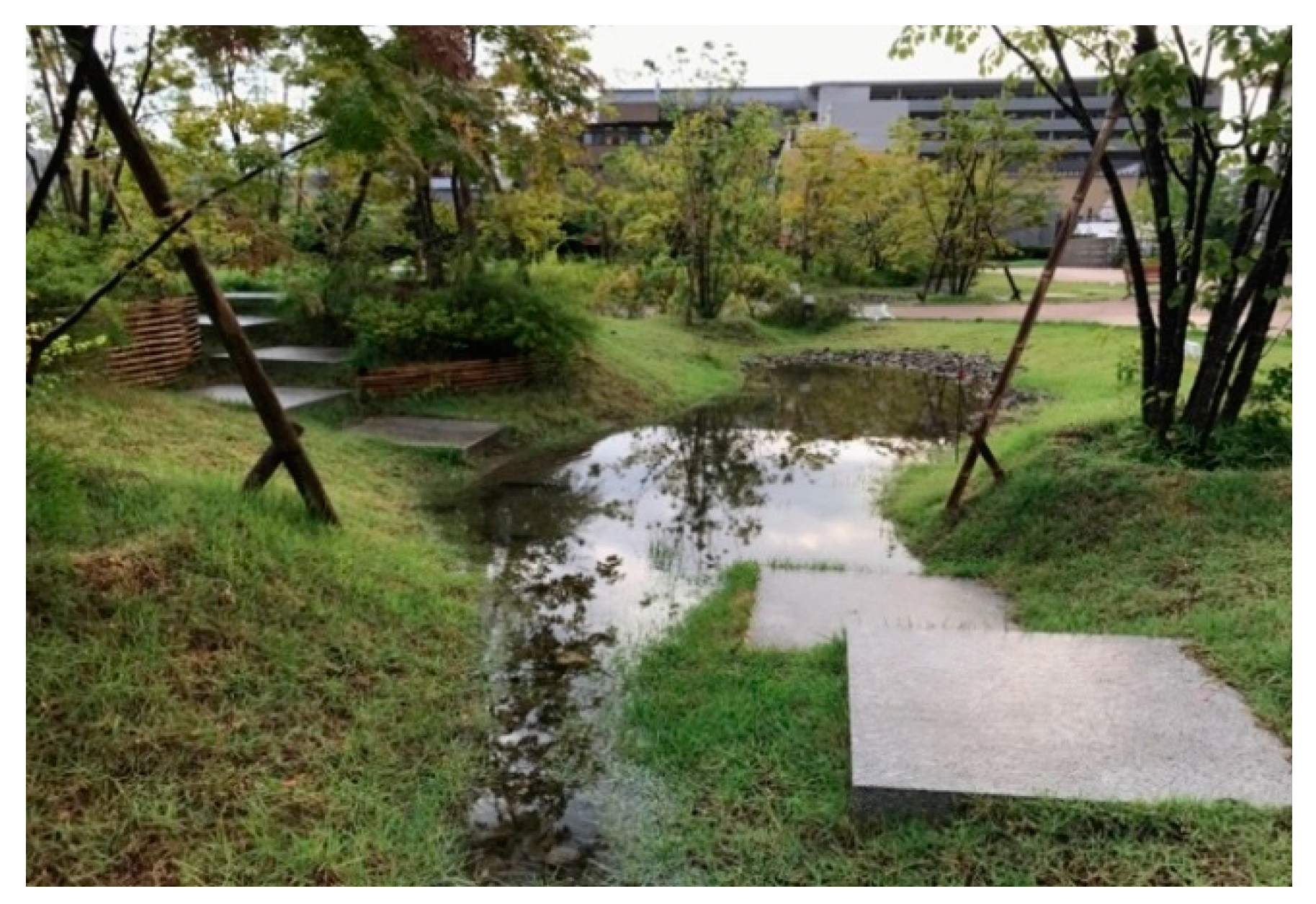
The surface appearance of rain gardens differs slightly from that of regular gardens. However, the particular plant configuration and soil structure are designed to support control of urban storm runoff, reduce peak flow, mitigate urban heat island effect, preserve biodiversity, purify rainwater and conserve groundwater [33,34]. Another appealing aspect of rain gardens is flexibility relating to physical dimensions and incorporation into the natural landscape, resulting in a wide application for residential areas, parking lots, roads), parks and other places requiring urban runoff control and pollutant removal [35,36,37,38,39,40]. Japan has introduced small-watershed rain gardens in recent years on university campuses (Figure 3) and elsewhere [41,42,43,44], but none in Kyoto’s Nakagyo Ward. There is a need to evaluate the effects of rain gardens on an urban catchment scale for promoting the green-movement approach of the rain garden and enhance ecosystem-related services to an urban area of Japan.
Against such a background, this research focused on the Nakagyo Ward area of Kyoto to evaluate the hydrological and water-quality effects of rain gardens with various rainfall return periods. The results are expected to help mitigate stormwater disaster hazards, enhance resistance against intense rainstorms and provide a scientific basis for urban planning in Kyoto and other worldwide cities with the same climate and rain garden construction conditions as Japan.
2. Materials and Methods
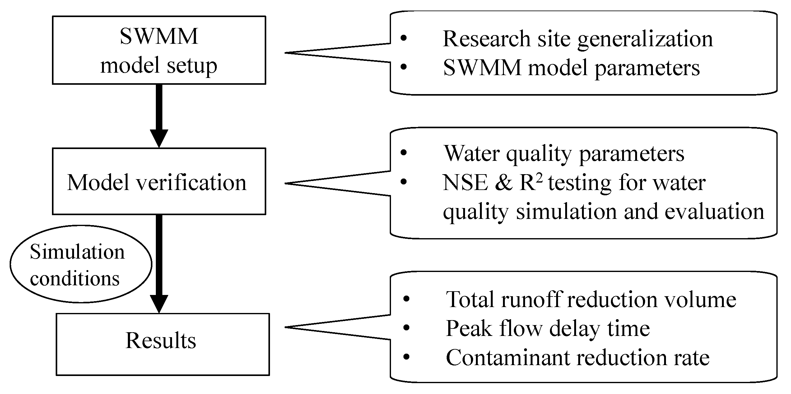
To evaluate the hydrological and water-quality control effects of rain gardens with various rainfall return periods, the total runoff reduction ratio, average peak flow delay time and contaminant reduction ratio were examined. Figure 4 shows the research steps:
- Model setup: generalization of research site and input of main parameters for ground surface and drainage systems;
- Model verification: comparison of monitored and simulated water quality for parameter validation;
Input of simulation conditions for result determination.
2.1. Research Site
The terrain of Kyoto’s central Nakagyo Ward, which is home to government offices, economic organizations, financial institutions and shopping centers, is mostly flat and slightly inclined to the southwest. It has a total area of 738 ha, with an average impervious ratio of 92.72% and an average slope of 1.18% based on GIS data from Ministry of Land, Infrastructure, Transport and Tourism of Japan [45]. Based on the Geospatial Information Authority of Japan’s detailed classifications for land use types, the research site consisted of 7 types of land use (Figure 5). In this study, we simplified the first and second types of middle/high-rise residential area (green and yellow zone in Figure 5) and the first type of residential area (lemon yellow zone in Figure 5) to the residential area, neighboring commercial area (red zone in Figure 5) and commercial area (pink zone in Figure 5) to the commercial area and quasi-industrial and industrial areas (mauve and blue zone in Figure 5) to the industrial area.
2.2. SWMM Model Setup
2.2.1. Model Description and Research Site Generalization
In this study, the EPA Storm Water Management Model (SWMM) was applied to simulate urban flood development. It is a dynamic rainfall-runoff model for long-term or single-event simulation of runoff quantities and qualities [19] used worldwide for planning, analysis and design related to stormwater runoff, combined and sanitary sewers and other drainage systems [46].
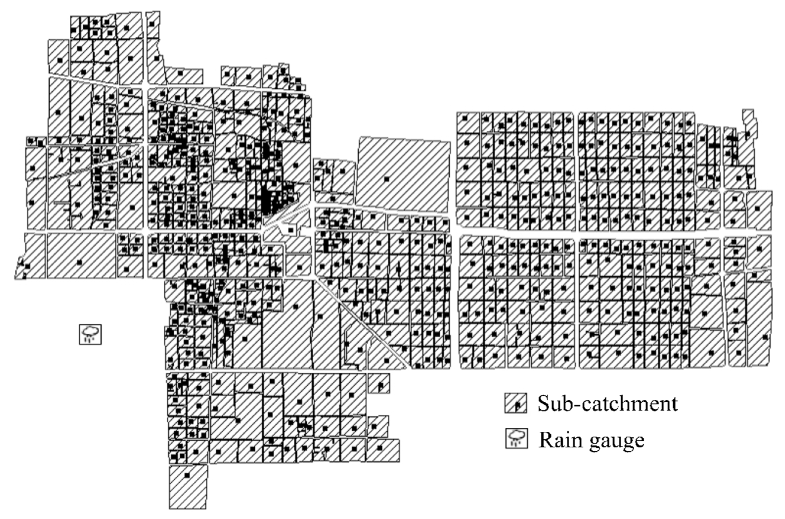
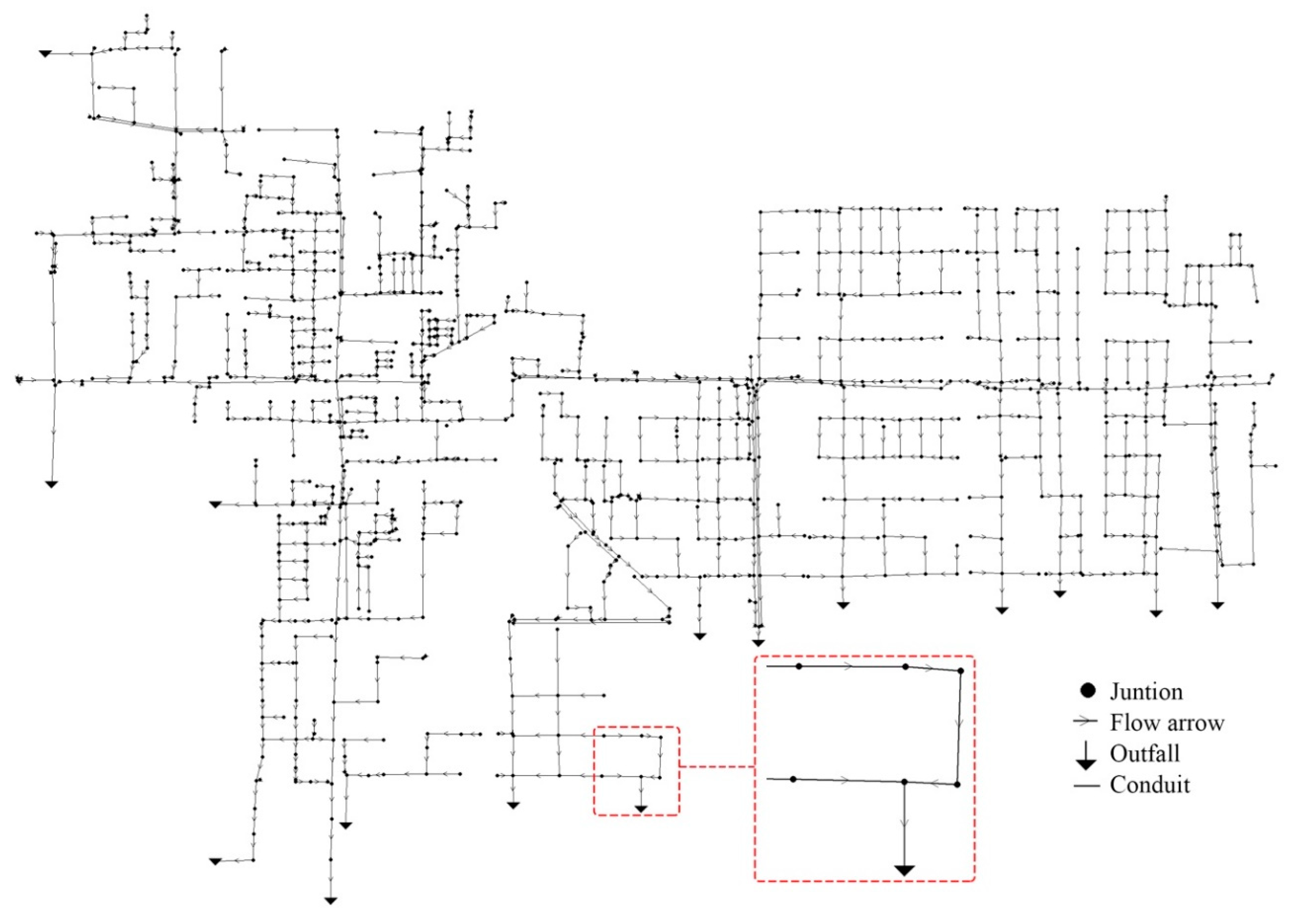
The sub-catchment and drainage systems are the fundamental units of the model. In this research, GIS data were obtained from Japan’s Ministry of Land, Infrastructure, Transport and Tourism [45] for generalization of the research site, and inp.PINS software was used to convert the relevant .shp file to .inp format. Pipe layouts were then drawn in the SWMM model based on data from the Kyoto City Water Supply and Sewage Bureau [47]. The generalized research site is shown in Figure 6, which has 642 sub-catchments over a total area of 607 ha and an rain gauge for inputting the rainfall data. The generalized drainage system is shown in Figure 7, which has 1149 junctions, 1192 conduits and 15 outfalls.
2.2.2. Model Parameters
The SWMM hydrological model requires numerous input parameters for the simulation process. The majority of these for definition of the ground surface and drainage system were derived using data from Japan’s Ministry of Land, Infrastructure, Transport and Tourism [45], the Kyoto City Water Supply and Sewage Bureau [47] and Google Maps (Table 2).
The remaining parameters were determined from the sub-catchment properties, including Manning’s N for impervious (N-Imperv) and pervious (N-Perv) areas, the depth of depression storage in impervious (Dstore-Imperv, mm) and pervious (Dstore-Perv, mm) areas, the percentage of impervious areas with no depression storage (%), the infiltration process and characteristic width. The infiltration process was treated with the Green-Ampt method, which assumes the presence of a sharp wetting front in the soil column, separating soil with initial moisture content below from saturated soil above [19]. The parameters were adjusted in line with the characteristics of each sub-catchment and the EPA SWMM User’s Manual [19] as listed in Table 3.
An initial estimate of characteristic width was made from the sub-catchment area divided by the average maximum overland flow length (i.e., the length of the flow path from the farthest drainage point of the sub-catchment before the flow becomes channelized) [19]. Zhou et al. [48] proposed a rational flow length range of 50–150 m and a corresponding flow time of 5–15 min. The Kyoto City Development Technology Standard [49] specifies an average flow time of 7 min for flat land, giving an estimated flow length of 70 m. Accordingly, the width of each sub-catchment area equals the area divided by the flow length (70 m).
The SWMM quality module requires definition of the pollutant build-up and wash-off processes for the three relevant land-use types. In this study, the exponential function for the build-up process was set as follows [19]:
here, is the amount of pollutant per unit area (kg/ha), is the maximum possible build-up (kg/ha), is the build-up rate constant (1/day) and is time (min).
Pollutant wash-off from a given land use category occurs during wet weather, and can be described as exponential wash-off, rating curve wash-off or event mean concentration. Rating curve wash-off and event mean concentration relate only to the influence of runoff on the flushing process, while exponential wash-off also involves consideration of influence from pollutant accumulation and rainfall-runoff on the flushing process. Accordingly, exponential wash-off was considered in this study as follows [19]:
here, is the wash load (kg/h), is the wash-off coefficient, is the runoff rate per unit area (mm/h), is the wash-off exponent and is pollutant buildup in mass units.
2.3. Model Implementation
2.3.1. Stormwater Sampling and Data Acquisition
A HOBO data-logging rain gauge (RG3-M) on the roof of Takakura Elementary School in the Nakagyo Ward area of Kyoto was used to monitor rainfall from 26 September to 26 October 2019. Runoff from typical rain falling from 4:50 p.m. to 6:30 p.m. on 3 October was tested to verify the model parameters. Storm runoff samples were collected from six drainage ditches (two for each of the C1, C2, N1, N2, R1 and R2 land-use types as indicated in Figure 5) near junctions at intervals of 5, 10, 15, 20, 30, 45, 60, 90 and 120 min. Natural rainfall samples collected using simple equipment near the rain gauge (Figure 8A) were stored in 500 mL polyethene bottles on site (Figure 8B) and transported to the Hydrological Environment Engineering Laboratory at Kyoto University for TSS, COD, TN and TP analysis. Supplementary Materials 1 shows the experimental details of the TSS, COD, TN and TP analysis. Due to different runoff start and end times, 9, 8, 6, 7, 8 and 10 samples were collected (at 5-min intervals) for the R1, R2, C1, C2, N1 and N2 plots, respectively. Thus, 49 samples (one natural rainfall and 48 runoff water) were used in water-quality testing.
2.3.2. Calibration and Validation of Parameters
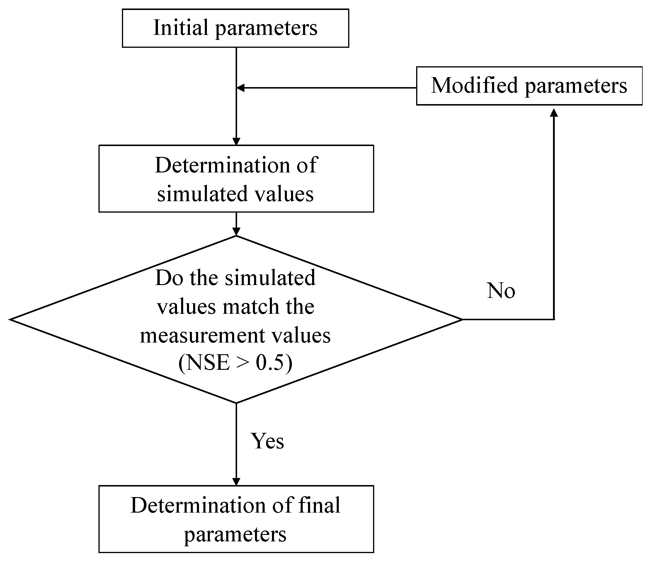
The initial parameters for the build-up and wash-off processes were determined from the observation data and results obtained by Li et al. [50] for the calibration process. The parameters were then inputted into the SWMM model to obtain the simulation values. The initial parameters were modified to match the measurement values, and the final parameters for validation were determined (Figure 9).
In validation, the R2 value and the Nash–Sutcliffe Efficiency coefficient (NSE) [51] were used as simulation indicators to validate the applied model quantitatively. The NSE equation was given as
here, (mg/L) represents the calculated concentration of TSS, COD, TN and TP at time i; (mg/L) represents the observed pollutant concentration at time i; (mg/L) represents the average observed pollutant concentration, and N represents the number of data points. NSE can range from −∞ to 1. If NSE > 0.5, the model simulation can be considered satisfactory [52].
2.4. Simulation Conditions
2.4.1. Design for Rainstorms with Different Return Periods
In the specific design rainstorm set as the primary condition for simulation, the famous Chicago method was used to create a short-duration storm hyetograph with six return periods. The method was proposed by Keifer and Chu [53] for calculation of design rainfall with urban stormwater infrastructures, and starts with an analytical and time-differentiable intensity-duration-frequency (IDF) equation [54]:
here, is average rainfall intensity (mm/min); is average rainfall intensity (L/s·ha); is the return period of the design rainfall (a); is the rainfall duration (min); , , and are local empirical parameters. is the rain force parameter, meaning the 1-min design rainfall (mm) for a return period of one year (a). is the rain force variation parameter (dimensionless), and is the rainfall duration correction parameter (a time constant (min) added to the curve after the logarithm of the storm intensity formula is iterated), and is the rain attenuation index, which is related to the return period.
Based on the rainfall intensity formula with different return periods published by the municipality of Kyoto (Table 4) [49], the parameters , , , are fitted using the least-squares method as shown in Table 5.
The method involves the use of two analytical equations for rainfall intensity over time—one valid before the peak and another valid after it—both deduced from the IDF analytical expression, preserving the same volumes of all rainfall intensities [55]. The time-to-peak ratio (0 < < 1) is generally introduced to describe the specific time of peak flow. The smaller the value of , the closer the peak flow is to the rainfall start time [41]. In this study, was set as 0.4.
Pre-peak rainfall intensity is calculated as follows [56]:
Post-peak intensity is calculated as follows [56]:
here, is the pre-peak rainfall duration, is the rain force parameter (meaning the 1-min design rainfall (mm) for a return period of one year (a), is the rain attenuation index value, is the rainfall duration correction parameter and is the time-to-peak ratio (0.4).
2.4.2. Rain Garden Parameters
An equally important input condition involves the rain garden setting parameters. In this study, those suggested by Zhang et al. [43] and the SWMM User’s Manual [19] were used (Table 6). The design rain gardens are one meter in depth, incorporating a soil thickness of 700 mm and a storage thickness of 300 mm. Moderately low runoff potential soil was set to ensure storage/infiltration functionality, with an average saturated hydraulic conductivity of 10.92 mm/h. The gardens were set up using the empirical method recommended by EPA, Razaei et al. [30] and Meng et al. [57], with 7% of each sub-catchment area a total of 42.68 ha.
3. Results
3.1. Parameter Calibration and Validation
The validated parameters of the build-up process are shown in Table 7. The maximum possible build-up values for TSS and COD were ranked as Industrial area > Commercial area > Residential area, and those for TN and TP as Commercial area > Residential area > Industrial area. The validated wash-off parameters are shown in Table 8. The wash-off coefficient and wash-off exponent for TSS, COD, TN and TP were ranked as Industrial area > Commercial area > Residential area.
The simulation indicator R2 and the NSE of TSS, COD, TN and TP at each plot are shown in Table 9. The lowest R2 value of 0.6645 was observed for TP at N1, and all NSE values exceeded 0.5, with the lowest at 0.6180. Accordingly, the applied model parameters (Table 7 and Table 8) can be considered appropriate.
3.2. Design Rainstorms with Different Return Periods
The design Chicago hyetograph with six return periods (3, 5, 10, 30, 50, 100 a) is shown in Figure 10. It is a two-hour representation with average rainfall intensities of 28.18, 32.81, 38.62, 50.19, 55.95 and 63.62 mm/h from 3, 5, 10, 30, 50 and 100-year return periods, respectively.
3.3. Total Runoff Reduction Ratios with Six Rainfall Return Periods
The total runoff volumes with and without rain gardens under scenarios with six rainfall return periods (Table 10) were all lower for the former. The reduction ratios from 3 a to 100 a were 13.78, 13.72, 13.68, 13.66, 13.61 and 12.11%, respectively, with the highest figure of 13.78% at 3 a. As the return period increases, the rate gradually decreases.
3.4. Peak Flow Delay Time with Six Rainfall Return Periods
The peak flow delay time with and without rain gardens for six rainfall return periods (Table 11) increased with the return period. However, values for all periods were the same at one minute. The maximum number of flooding nodes (with/without rain gardens) was observed at 30 a. We used the reduction of flooding nodes to verify the function of the rain gardens. The flooding nodes reduction value from 3a to 5a increased, and the value from 5a to 100a decreased, with a maximum value at 5 a.
3.5. Contaminant Reduction Rate with Six Rainfall Return Periods
The contaminant reduction rate with six rainfall return periods (Table 12) shows a gradual reduction as the return period increases. The maximum rates for TSS, COD, TN and TP were observed at 3 a (15.50, 16.17, 17.34 and 19.07%, respectively).
4. Discussion
4.1. Total Runoff Reduction Rate with Six Rainfall Return Periods
The study results showed that runoff volume reductions of 13.78, 13.72, 13.68, 13.66, 13.61 and 12.11% were achieved by adding rain garden facilities with different rainfall return periods in Nakagyo Ward. Zhang et al. [43] also reported that more than 60% of runoff was controlled by two rain gardens at Kyoto Gakuen University (KGU). The runoff control rate observed in this study was significantly lower than that observed by Zhang et al. [43] due to differences between the rain garden areas and rainfall conditions. In this study, the ratio of the rain garden facilities to the catchment area was 7.03%, which is much lower than the 91.25% of Zhang et al. [43]. Meanwhile, the maximum rainfall intensity of Zhang et al. [43] was 13.91 mm/h, which is less than the minimum rainfall intensity of this study (28.18 mm/h).
Li et al. [50] evaluated the runoff reduction ratio of different combined low-impact development (LID) scenarios with 26 mm/h rainfall conditions. The area of scenario three accounts for 9.8% of the total area, which is closer to the parameters of this study (7.03% of the total sub-catchments). Their results showed a 17.8% runoff volume for this scenario. In this study, the runoff reduction rate at 3 a (average rainfall intensity: 28.18 mm/h) was 13.78%. It was lower than the value observed by Li et al. [50], mainly due to their use of different combined LID facilities, while only rain gardens were involved in this study. Although the 92.72% impervious ratio limited the settable range of rain gardens, the overall runoff reduction ratio was still evident at 3 a (13.78%).
4.2. Peak Flow Delay Time with Six Rainfall Return Periods
The results of Li et al. [50] showed a one-minute peak flow delay time in scenario three with a rainfall intensity of 26 mm/h, which is consistent with the findings of this study (one minute for a rainfall intensity of 28.18 mm/h). Schlea et al. [58] reported that street-side rain gardens in Ohio, USA, had a peak delay time of 16 min; Li et al. [59] reported a time of 6 min for rain gardens in Xi’an, China, with a 10-year return period; and Zhang et al. [44] reported a time of around two hours for a rain garden at KGU with a rainfall intensity of 15–50 mm/h. However, in this study, the peak flow delay time was only one minute for a rainfall intensity of 28–64 mm/h. In the research of Zhang et al. [44], the rain garden area was 409 m2 with a catchment area of 300 m2. In this study, the rain garden area was 43 ha with a catchment area of 607 ha. The root cause of the different peak flow delay times is the different setting parameters, including surface properties, soil properties and drainage properties. The findings of Qin et al. [60] indicated that LID performance is affected by structure and properties, which also confirmed this conjecture.
This study (Table 11) indicated a one-minute peak delay time with a 100-year return period, reflecting the positive runoff control effect of the rain gardens in Nakagyo Ward.
Table 10 shows that the maximum number of flooding nodes was observed at 30 a rather than 100 a. We analyzed the flooding node data and found that the reason is the algorithm and random ratio of SWMM itself. The unit of flooding time of the model is the hour. When the flooding time exceeded the minimum value of 0.01 h (36 s), the node became the flooding type. At 30 a and 100 a, 357 and 309 nodes had a flood time of 36 s. If we set the flooding time to 37 s, there was 305 flooded nodes at 30 a, and 329 nodes at 100 a, which confirmed our hypothesis that flooding nodes gradually increase with the increase in return period. Meanwhile, the specific calculation method of the flooding time in the algorithm needs further study.
When rainfall intensity increased to a certain level, the function of the rain gardens became saturated. The maximum flooding nodes reduction was observed at 5 a (Table 11), demonstrating the capacity of the rain gardens to competently handle the rainfall intensity of a five-year return period (32.81 mm/h). After the rain garden function becomes saturated, the number of flood nodes cannot be effectively reduced, thus the number of flood nodes gradually approaches the value of “Total flooding nodes (without RG)”. Therefore, the flooding node reduction gradually decreased from 5 a to 100 a, which indicated that the rain gardens do not have an excellent flood node control effect for heavy rainstorms.
4.3. Contaminant Reduction with Six Rainfall Return Periods
Li et al. [50] reported that the TSS, COD, TN and TP reduction ratios for scenario three with a rainfall intensity of 26 mm/h were 19.7, 19.2, 18.6 and 16.9%, respectively. In this study, the corresponding ratios at 3 a (average rainfall intensity: 28.18 mm/h) were broadly similar at 15.5, 16.17, 17.34 and 19.07%.
The laboratory test of Davis et al. [61] showed that the TN and TP removal ratios of rain gardens on urban rainwater runoff reached 55–55% and 70–85%. Jiang et al. [38] conducted a field study of two small rain gardens (each 24 m2), and showed average reduction ratios of 51.79, 39.8, 56.84 and 56.99% for TSS, COD, TN and TP, respectively. Laboratory testing and field study results showed much higher reduction ratios for rain gardens. It may be attributable to the different structures and properties of rain garden facilities; further research needs to be conducted in Nakagyo Ward for verification.
Although contaminant reduction ratios gradually decreased with the increase in return periods, even with the period of 100 a there were still TSS, COD, TN and TP removal ratios of 13.00, 12.90, 12.83 and 14.03%. Accordingly, the rain gardens in Nakagyo Ward can generally be considered to have a positive pollutant removal effect.
5. Conclusions
This study involved simulation and evaluation of the hydrological and water-quality purification effects of rain garden facilities in the Nakagyo Ward area of Kyoto in Japan. The SWMM model was used for simulation under design short rainstorm conditions with six rainfall return periods. The significant findings can be summarized as follows:
- (1)
- The gardens exhibited a positive runoff control effect. Although the 92.72% impervious ratio limited the settable range of the facilities, an overall runoff reduction rate was apparent (13.78%) with an average rainfall intensity of 28.18 mm/h.
- (2)
- The gardens were a valid option for flood mitigation. There was still a one-minute delay time even for the 100-year return period with an average rainfall intensity of 63.62 mm/h.
- (3)
- The gardens exhibited significant contaminant reduction ratios for the three-year return period in particular (TSS 15.50%, COD 16.17%, TN 17.34%, TP 19.07%).
Overall, the Nakagyo Ward rain gardens can be considered practical in reducing stormwater disaster risk and enhancing resistance against short-term rainstorms. These facilities may be considered for urban planning in Kyoto and other worldwide cities with the same climate and rain garden construction conditions as Japan.
Supplementary Materials
The following are available online at https://0-www-mdpi-com.brum.beds.ac.uk/2071-1050/12/23/9982/s1.
Author Contributions
L.Z. and S.S. conceived and designed the research; L.Z. and Z.Y. collected and analyzed the data; L.Z. drafted the manuscript and prepared figures; L.Z., Z.Y., and S.S. discussed the results and revised the manuscript. All authors have read and agreed to the published version of the manuscript.
Funding
This study was funded by a Grant-in-Aid for Scientific Research (B) from the Japan Society for the Promotion of Science (18H02226).
Acknowledgments
The authors are grateful to Kimihito Nakamura at the Laboratory of Hydrological Environment Engineering in Kyoto University’s Department of Agriculture for providing guidance and help in the hydrology and water-quality testing aspects of the research.
Conflicts of Interest
The authors declare no conflict of interest.
References
- Hostetler, M.E.; Allen, W.; Meurk, C. Conserving urban biodiversity? Creating green infrastructure is only the first step. Landsc. Urban Plan. 2011, 100, 369–371. [Google Scholar] [CrossRef]
- Beninde, J.; Veith, M.; Hochkirch, A. Biodiversity in cities needs space: A meta-analysis of factors determining intra-urban biodiversity variation. Ecol. Lett. 2015, 18, 581–592. [Google Scholar] [CrossRef] [PubMed]
- Baek, S.-S.; Choi, D.-H.; Jung, J.-W.; Lee, H.-J.; Lee, H.; Yoon, K.-S.; Cho, K.H. Optimizing low impact development (LID) for stormwater runoff treatment in urban area, Korea: Experimental and modeling approach. Water Res. 2015, 86, 122–131. [Google Scholar] [CrossRef] [PubMed]
- Konrad, C.; Booth, D.B.; Burges, S.J. Effects of urban development in the Puget Lowland, Washington, on interannual streamflow patterns: Consequences for channel form and streambed disturbance. Water Resour. Res. 2005, 41, 1–15. [Google Scholar] [CrossRef]
- Chen, Y.; Zhou, H.; Zhang, H.; Du, G.; Zhou, J. Urban flood risk warning under rapid urbanization. Environ. Res. 2015, 139, 3–10. [Google Scholar] [CrossRef]
- Thorne, C.R.; O’Donnell, E.C.; Ozawa, C.P.; Hamlin, S.; Smith, L.A. Overcoming uncertainty and barriers to adoption of Blue-Green Infrastructure for urban flood risk management. J. Flood Risk Manag. 2018, 11, S960–S972. [Google Scholar] [CrossRef]
- Luo, K.; Hu, X.; Zhengsong, W.; Wu, Z.; Cheng, H.; Hu, Z.; Mazumder, A. Impacts of rapid urbanization on the water quality and macroinvertebrate communities of streams: A case study in Liangjiang New Area, China. Sci. Total Environ. 2018, 621, 1601–1614. [Google Scholar] [CrossRef]
- Wang, R.; Kalin, L. Combined and synergistic effects of climate change and urbanization on water quality in the Wolf Bay watershed, southern Alabama. J. Environ. Sci. 2018, 64, 107–121. [Google Scholar] [CrossRef]
- Tsuchiya, S. Factualization and Discussion on “Urbanization Rate” in Japan—From the Viewpoint of Regional Economy. Available online: https://www.boj.or.jp/research/wps_rev/wps_2009/data/wp09j04.pdf (accessed on 15 November 2020).
- Shimizu, H. Observation and categorization of land use and population/household change in whole Japanese land by using third standard grid cell data. J. City Plan. Inst. Jpn. 2015, 50. [Google Scholar] [CrossRef]
- Kyoto Regional Meteorological Observatory. Heavy Rain in Kyoto Prefecture from 15 to 17 August 2014. Available online: https://www.jma-net.go.jp/kyoto/2_data/report/doc/kishousokuhou20140818.pdf (accessed on 15 November 2020).
- Kimura, S.; Ishikawa, Y.; Katada, T.; Asano, K.; Sato, H. The Structural Analysis of Economic Damage of Offices by Flood Disasters in Urban Areas. Doboku Gakkai Ronbunshuu D 2007, 63, 88–100. [Google Scholar] [CrossRef]
- Baba, K.; Matsuura, M.; Shinoda, S.; Hijioka, Y.; Shirai, N.; Tanaka, M. A Policy Recommendation of Climate Change Adaptation in Disaster Risk Reduction Based on Stakeholder Analysis—A Case Study on Urban Flood Damage in Tokyo. J. Jpn. Soc. Civ. Eng. Ser. G Environ. Res. 2012, 68. [Google Scholar] [CrossRef] [Green Version]
- Takeda, M.; Takahashi, T.; Nagao, Y.; Hirayama, Y.; Matsuo, N. The Examination on the Inundation Analysis Model Due to Interior Runoff in Urban Area and Its Application to the Countermeasures in Flood Situation. J. Jpn. Soc. Civ. Eng. Ser. B1 Hydraul. Eng. 2012, 68. [Google Scholar] [CrossRef] [Green Version]
- Kawakubo, S.; Tanaka, M.; Baba, K. Resilience Assessment of Major Japanese Cities Based on Public Statistical Information. Soc. Environ. Sci. Jpn. 2017, 30, 215–224. [Google Scholar] [CrossRef]
- Prince George’s County. Design Manual for Use of Bioretention in Stormwater Management; Watershed Protection Branch: Landover, MD, USA, 1993.
- Dietz, M.E.; Clausen, J.C. A Field Evaluation of Rain Garden Flow and Pollutant Treatment. Water Air Soil Pollut. 2005, 167, 123–138. [Google Scholar] [CrossRef]
- Xiang, L.; Li, J.; Kuang, N.; Che, W.; Li, Y.; Liu, X. Discussion on the design methods of rainwater garden. Water Wastewater Eng. 2008, 34, 47–51. [Google Scholar] [CrossRef]
- EPA. SWMM User’s Manual Version 5.1. Available online: https://www.epa.gov/sites/production/files/2019-02/documents/epaswmm5_1_manual_master_8-2-15.pdf (accessed on 15 November 2020).
- Yu, S.L.; Kuo, J.-T.; Fassman, E.A.; Pan, H. Field Test of Grassed-Swale Performance in Removing Runoff Pollution. J. Water Resour. Plan. Manag. 2001, 127, 168–171. [Google Scholar] [CrossRef]
- Hunt, W.F.; Jarrett, A.R.; Smith, J.T.; Sharkey, L.J. Evaluating Bioretention Hydrology and Nutrient Removal at Three Field Sites in North Carolina. J. Irrig. Drain. Eng. 2006, 132, 600–608. [Google Scholar] [CrossRef]
- Guo, C.; Li, J.; Li, H.; Li, Y. Influences of stormwater concentration infiltration on soil nitrogen, phosphorus, TOC and their relations with enzyme activity in rain garden. Chemosphere 2019, 233, 207–215. [Google Scholar] [CrossRef]
- Hatt, B.E.; Fletcher, T.D.; Deletic, A. Hydrologic and pollutant removal performance of stormwater biofiltration systems at the field scale. J. Hydrol. 2009, 365, 310–321. [Google Scholar] [CrossRef]
- Chapman, C.; Horner, R.R. Performance Assessment of a Street-Drainage Bioretention System. Water Environ. Res. 2010, 82, 109–119. [Google Scholar] [CrossRef]
- Gülbaz, S.; Kazezyılmaz-Alhan, C.M. Experimental Investigation on Hydrologic Performance of LID with Rainfall-Watershed-Bioretention System. J. Hydrol. Eng. 2017, 22, 4016003. [Google Scholar] [CrossRef]
- Davis, A.P. Field Performance of Bioretention: Water Quality. Environ. Eng. Sci. 2007, 24, 1048–1064. [Google Scholar] [CrossRef]
- Line, D.E.; Hunt, W.F. Performance of a Bioretention Area and a Level Spreader-Grass Filter Strip at Two Highway Sites in North Carolina. J. Irrig. Drain. Eng. 2009, 135, 217–224. [Google Scholar] [CrossRef]
- Li, H.; Davis, A.P. Water Quality Improvement through Reductions of Pollutant Loads Using Bioretention. J. Environ. Eng. 2009, 135, 567–576. [Google Scholar] [CrossRef]
- Liu, Y.; Bralts, V.F.; Engel, B. Evaluating the effectiveness of management practices on hydrology and water quality at watershed scale with a rainfall-runoff model. Sci. Total Environ. 2015, 511, 298–308. [Google Scholar] [CrossRef] [PubMed]
- Rezaei, A.R.; Ismail, Z.; Niksokhan, M.H.; Dayarian, M.A.; Ramli, A.H.; Shirazi, S.M. A Quantity–Quality Model to Assess the Effects of Source Control Stormwater Management on Hydrology and Water Quality at the Catchment Scale. Water 2019, 11, 1415. [Google Scholar] [CrossRef] [Green Version]
- Dagenais, D.; Brisson, J.; Fletcher, T.D. The role of plants in bioretention systems; does the science underpin current guidance? Ecol. Eng. 2018, 120, 532–545. [Google Scholar] [CrossRef]
- Osman, M.; Yusof, K.W.; Takaijudin, H.; Goh, H.; Malek, M.A.; Azizan, N.A.; Ghani, A.A.; Abdurrasheed, A.S. A Review of Nitrogen Removal for Urban Stormwater Runoff in Bioretention System. Sustainability 2019, 11, 5415. [Google Scholar] [CrossRef] [Green Version]
- Huang, Z.; Xiao, J.; Liu, B. Analysis on Rain Garden. J. Anhui Agric. Sci. 2011, 39, 5412–5413. [Google Scholar] [CrossRef]
- Morimoto, Y. Rain Garden Revives the City; Nikkei Business Publication Inc.: Tokyo, Japan, 2017; pp. 134–143. (In Japanese) [Google Scholar]
- Asleson, B.C.; Nestingen, R.S.; Gulliver, J.S.; Hozalski, R.M.; Nieber, J.L. Performance Assessment of Rain Gardens. JAWRA J. Am. Water Resour. Assoc. 2009, 45, 1019–1031. [Google Scholar] [CrossRef]
- Good, J.F.; O’Sullivan, A.D.; Wicke, D.; Cochrane, T. Contaminant removal and hydraulic conductivity of laboratory rain garden systems for stormwater treatment. Water Sci. Technol. 2012, 65, 2154–2161. [Google Scholar] [CrossRef] [PubMed]
- Komlos, J.; Traver, R.G. Long-Term Orthophosphate Removal in a Field-Scale Storm-Water Bioinfiltration Rain Garden. J. Environ. Eng. 2012, 138, 991–998. [Google Scholar] [CrossRef]
- Jiang, C.; Li, J.; Li, H.; Li, Y.; Chen, L. Field Performance of Bioretention Systems for Runoff Quantity Regulation and Pollutant Removal. Water Air Soil Pollut. 2017, 228, 468. [Google Scholar] [CrossRef]
- Hong, J.; Geronimo, F.K.; Choi, H.; Kim, L.-H. Impacts of nonpoint source pollutants on microbial community in rain gardens. Chemosphere 2018, 209, 20–27. [Google Scholar] [CrossRef] [PubMed]
- Kim, J.; Lee, J.; Song, Y.H.; Han, H.; Joo, J.G. Modeling the Runoff Reduction Effect of Low Impact Development Installations in an Industrial Area, South Korea. Water 2018, 10, 967. [Google Scholar] [CrossRef] [Green Version]
- Yamada, S.; Shibata, S. Quantitative evaluation about rainwater-runoff characteristics of rain garden. J. Jpn. Soc. Reveg. Technol. 2017, 43, 251–254. [Google Scholar] [CrossRef] [Green Version]
- Watanabe, Y.; Yonemura, S.; Hirano, T.; Zhang, L.; Shibata, S. Field evaluation of rain gardens for reducing stormwater runoff. Archit. Inst. Jpn. Acad. Lect. Collect. Summ. 2018, 641–642. [Google Scholar]
- Zhang, L.; Oyake, Y.; Morimoto, Y.; Niwa, H.; Shibata, S. Rainwater storage/infiltration function of rain gardens for management of urban storm runoff in Japan. Landsc. Ecol. Eng. 2019, 15, 421–435. [Google Scholar] [CrossRef]
- Zhang, L.; Oyake, Y.; Morimoto, Y.; Niwa, H.; Shibata, S. Flood mitigation function of rain gardens for management of urban storm runoff in Japan. Landsc. Ecol. Eng. 2020, 16, 223–232. [Google Scholar] [CrossRef]
- Sakamoto, J.; Hara, T. Analysis of the Actual Situation of the Local Civil Engineering Consultant Companies Since the Great East Japan Earthquake: Focusing on the Bid Information of Ministry of Land, Infrastructure, Transport and Tourism, Japan. J. Jpn. Soc. Civ. Eng. Ser. Constr. Manag. 2018, 74. [Google Scholar] [CrossRef]
- EPA. Storm Water Management Model (SWMM). Available online: https://www.epa.gov/water-research/storm-water-management-model-swmm (accessed on 15 November 2020).
- Kyoto City Water Supply and Sewage Bureau. Available online: http://www.kyoto-gesuido.jp/SuperaPageWeb.aspx# (accessed on 15 November 2020).
- Zhou, Y.; Yu, M.; Chen, Y. Estimation of Sub-Catchment Width in SWMM. China Water Wastewater 2014, 30, 61–64. [Google Scholar]
- Kyoto City Development Technology Standard. Available online: https://www.city.kyoto.lg.jp/tokei/cmsfiles/contents/0000197/197400/gizyutukizyunn(H280325).pdf (accessed on 15 November 2020).
- Li, Q.; Wang, F.; Yu, Y.; Huang, Z.; Li, M.; Guan, Y. Comprehensive performance evaluation of LID practices for the sponge city construction: A case study in Guangxi, China. J. Environ. Manag. 2019, 231, 10–20. [Google Scholar] [CrossRef] [PubMed]
- Nash, J.E.; Sutcliffe, J.V. River flow forecasting through conceptual models part I—A discussion of principles. J. Hydrol. 1970, 10, 282–290. [Google Scholar] [CrossRef]
- Moriasi, D.N.; Arnold, J.G.; Van Liew, M.W.; Bingner, R.L.; Harmel, R.D.; Veith, T.L. Model Evaluation Guidelines for Systematic Quantification of Accuracy in Watershed Simulations. Trans. ASABE 2007, 50, 885–900. [Google Scholar] [CrossRef]
- Keifer, C.J.; Chu, H.H. Synthetic storm pattern for drainage design. J. Hydraul. Div. 1957, 83, 1–25. [Google Scholar]
- Bai, Y.; Zhao, N.; Zhang, R.; Zeng, X. Storm Water Management of Low Impact Development in Urban Areas Based on SWMM. Water 2018, 11, 33. [Google Scholar] [CrossRef] [Green Version]
- Da Silveira, A.L.L. Cumulative equations for continuous time Chicago hyetograph method. RBRH 2016, 21, 646–651. [Google Scholar] [CrossRef]
- Dai, Y.; Wang, Z.; Dai, L.; Cao, Q.; Wang, T. Application of Chicago Hyetograph Method in Design of Short Duration Rainstorm Pattern. J. Arid Meteorol. 2017, 35, 1061–1069. [Google Scholar] [CrossRef]
- Meng, Y.; Chen, J.; Zhang, S. Research status of bio-retention technology and discussion on key problems on its domestic application. China Water Wastewater 2010, 24, 20–24. [Google Scholar]
- Schlea, D.; Martin, J.F.; Ward, A.D.; Brown, L.C.; Suter, S.A. Performance and Water Table Responses of Retrofit Rain Gardens. J. Hydrol. Eng. 2014, 19, 05014002. [Google Scholar] [CrossRef]
- Li, J.; Li, Y.; Li, Y. SWMM-based evaluation of the effect of rain gardens on urbanized areas. Environ. Earth Sci. 2015, 75, 1–14. [Google Scholar] [CrossRef]
- Qin, H.-P.; Li, Z.-X.; Fu, G. The effects of low impact development on urban flooding under different rainfall characteristics. J. Environ. Manag. 2013, 129, 577–585. [Google Scholar] [CrossRef] [PubMed] [Green Version]
- Davis, A.P.; Shokouhian, M.; Sharma, H.; Minami, C. Water Quality Improvement through Bioretention Media: Nitrogen and Phosphorus Removal. Water Environ. Res. 2006, 78, 284–293. [Google Scholar] [CrossRef] [PubMed]
Figure 1.
Urban flooding in Nakagyo Ward, Kyoto. (A) Submerged Marutamachi Street near Kyoto Gyoin; (B) flooding in Shijo subway station. (Source: https://matome.naver.jp/odai/2140819136800299801?&page=1).
Figure 1.
Urban flooding in Nakagyo Ward, Kyoto. (A) Submerged Marutamachi Street near Kyoto Gyoin; (B) flooding in Shijo subway station. (Source: https://matome.naver.jp/odai/2140819136800299801?&page=1).

Figure 2.
Diagram of a typical rain garden structure.

Figure 3.
Rain garden at Kyoto Gakuen University, Nishigyo Ward, Kyoto, Japan [43].
Figure 3.
Rain garden at Kyoto Gakuen University, Nishigyo Ward, Kyoto, Japan [43].

Figure 4.
Research steps.

Figure 5.
Location and land use in Nakagyo Ward, Kyoto, Japan. (Source: https://cityzone.mapexpert.net).
Figure 5.
Location and land use in Nakagyo Ward, Kyoto, Japan. (Source: https://cityzone.mapexpert.net).

Figure 6.
Generalized sub-catchment area.

Figure 7.
Generalized drainage system.

Figure 8.
Rainwater collection equipment and on-site runoff collection. (A) Rainwater collection equipment near the rain gauge; (B) on-site runoff collection.
Figure 8.
Rainwater collection equipment and on-site runoff collection. (A) Rainwater collection equipment near the rain gauge; (B) on-site runoff collection.

Figure 9.
Model calibration and validation.

Figure 10.
Design Chicago hyetograph with six return periods.


Table 1.
Summary of percent runoff and pollutant retention by rain gardens.
| Location | Runoff | TSS | TN | TP | COD | Evaluation Methods | Study |
|---|---|---|---|---|---|---|---|
| North Carolina, USA | 78 | - | 40 | 65 | - | Field sampling and laboratory analysis | [21] |
| Xi’an, China | 97 | - | - | - | - | Runoff sampling and laboratory analysis | [22] |
| Melbourne, Australia | 33 | - | - | - | - | Field sampling and laboratory analysis | [23] |
| Washington, USA | 48–74 | 87–93 | - | 67–83 | - | Event-based, flow-paced composite sampling and laboratory analysis | [24] |
| Istanbul, Turkey | 23–85 | - | - | - | - | Field sampling and laboratory analysis | [25] |
| Maryland, USA | - | 22 | - | 74 | - | Field sampling and laboratory analysis | [26] |
| North Carolina, USA | - | 83 | 62 | 48 | - | Refrigerated auto-sampling and laboratory analysis | [27] |
| Maryland, USA | - | 93 | - | 90 | - | Refrigerated auto-sampling and laboratory analysis | [28] |
| Indiana, USA | 26 | 54 | 34 | 47 | 28 | L-THIA-LID 2.1 model | [29] |
| Kuala Lumpur, Malaysia | 23 | 41 | 29 | - | - | Storm Water Management Model (SWMM) | [30] |
Table 2.
SWMM parameters and sources.
| Type | Parameter | Source |
|---|---|---|
| Sub-catchment | Spatial location, area, slope, Impervious ratio | Ministry of Land, Infrastructure, Transport and Tourism, Japan [45]; Google Maps |
| Junction | Spatial location, invert elevation, maximum depth | Kyoto City Water Supply and Sewage Bureau [47] |
| Conduit | Spatial location, shape, diameter, length | Kyoto City Water Supply and Sewage Bureau [47] |
| Outfall | Spatial location, depth | Kyoto City Water Supply and Sewage Bureau [47] |
Table 3.
Parameters for sub-catchment properties.
| Parameter | Value | |
|---|---|---|
| Manning’s n | N-Imperv | 0.01 |
| N-Perv | 0.1 | |
| Depth of depression storage | Dstore-Imperv | 0.05 (mm) |
| Dstore-Perv | 0.05 (mm) | |
| Green-Ampt | Suction head | 3.0 (mm) |
| Conductivity | 0.5 (mm/h) | |
| Initial deficit | 4 | |
| Percentage of impervious areas with no depression storage | 25 (%) | |
Table 4.
Rainfall intensity formula for Kyoto with six return periods (year).
| Return Period | 3 a | 5 a | 10 a | 30 a | 50 a | 100 a |
|---|---|---|---|---|---|---|
| Rainfall intensity formula (Kyoto) |
Table 5.
Fitted , , and parameters with six return periods (year).
| Return Period | 3 a | 5 a | 10 a | 30 a | 50 a | 100 a |
|---|---|---|---|---|---|---|
| A | 0.146 | 0.146 | 0.144 | 0.143 | 0.142 | 0.140 |
| C | 73.164 | 57.666 | 47.186 | 39.287 | 37.118 | 34.461 |
| b | 3.580 | 3.812 | 4.182 | 5.668 | 6.356 | 7.717 |
| n | 0.500 | 0.498 | 0.493 | 0.477 | 0.470 | 0.457 |
| R2 | 0.997 | 0.998 | 0.998 | 0.998 | 0.998 | 0.998 |
Table 6.
Rain garden parameters.
| Surface | Berm height | Vegetation volume fraction | Surface roughness | Surface slope |
| 150 mm | 0 | 0 | 0 | |
| Soil | Soil thickness | Soil porosity | Field capacity | Wilting point |
| 700 mm | 0.453 | 0.19 | 0.085 | |
| Conductivity | Conductivity slope | Suction head | ||
| 10.92 mm/h | 50 | 109.2 mm | ||
| Storage | Storage thickness | Void ratio | Seepage rate | Storage clogging factor |
| 300 mm | 0.75 | 10.92 mm/h | 0 | |
| Drain | Flow coefficient | Flow exponent | Offset height | |
| 0 | 0.5 | 6 mm |
Table 7.
Coefficients of the pollutant build-up process.
| Coefficient | TSS | COD | TN | TP | |
|---|---|---|---|---|---|
| Residential areas | C1 | 53 | 10 | 8 | 0.5 |
| C2 | 10 | 10 | 10 | 10 | |
| Commercial areas | C1 | 65 | 15 | 9 | 0.7 |
| C2 | 10 | 10 | 10 | 10 | |
| Industrial areas | C1 | 95 | 20 | 5 | 0.2 |
| C2 | 10 | 10 | 10 | 10 |
Notes: C1 is the maximum possible build-up (kg/ha). C2 is the build-up rate constant (1/day).
Table 8.
Coefficients of the pollutant wash-off process.
| Coefficient | TSS | COD | TN | TP | |
|---|---|---|---|---|---|
| Residential areas | S1 | 0.007 | 0.0035 | 0.002 | 0.001 |
| S2 | 1.5 | 1.5 | 1.5 | 1.5 | |
| Commercial areas | S1 | 0.008 | 0.004 | 0.003 | 0.002 |
| S2 | 1.7 | 1.7 | 1.7 | 1.7 | |
| Industrial areas | S1 | 0.009 | 0.005 | 0.004 | 0.003 |
| S2 | 1.8 | 1.8 | 1.8 | 1.8 |
Notes: S1 is the wash-off coefficient. S2 is the wash-off exponent.
Table 9.
R2 and Nash–Sutcliffe Efficiency coefficient (NSE) values for TSS, COD, TN and TP at each plot.
Table 9.
R2 and Nash–Sutcliffe Efficiency coefficient (NSE) values for TSS, COD, TN and TP at each plot.
| TSS | COD | TN | TP | ||
|---|---|---|---|---|---|
| R1 | R2 | 0.8499 | 0.7363 | 0.8266 | 0.7652 |
| NSE | 0.6448 | 0.6237 | 0.7768 | 0.7539 | |
| R2 | R2 | 0.8386 | 0.7815 | 0.8053 | 0.8466 |
| NSE | 0.6613 | 0.6637 | 0.7963 | 0.8205 | |
| C1 | R2 | 0.8601 | 0.8802 | 0.8506 | 0.8132 |
| NSE | 0.6309 | 0.6062 | 0.8141 | 0.6496 | |
| C2 | R2 | 0.8318 | 0.7252 | 0.7198 | 0.7721 |
| NSE | 0.7267 | 0.6211 | 0.6180 | 0.6376 | |
| N1 | R2 | 0.8667 | 0.7101 | 0.8065 | 0.6645 |
| NSE | 0.6272 | 0.6147 | 0.6273 | 0.6581 | |
| N2 | R2 | 0.8474 | 0.7116 | 0.8523 | 0.8065 |
| NSE | 0.6271 | 0.6565 | 0.7008 | 0.8011 |
Table 10.
Total runoff volumes for six rainfall return periods.
| Return Period (a) | Without Rain Gardens (106 L) | With Rain Gardens (106 L) | Reduction Ratio (%) |
|---|---|---|---|
| 3 | 337.76 | 291.20 | 13.78 |
| 5 | 394.07 | 340.00 | 13.72 |
| 10 | 465.14 | 401.52 | 13.68 |
| 30 | 606.27 | 523.48 | 13.66 |
| 50 | 676.57 | 584.49 | 13.61 |
| 100 | 770.33 | 677.09 | 12.11 |
Table 11.
Peak flow time and flooding nodes with and without rain gardens (RG) for six rainfall return periods.
Table 11.
Peak flow time and flooding nodes with and without rain gardens (RG) for six rainfall return periods.
| Return Period (a) | Average Hours of Peak Flow Without RG (min) | Average Hours of Peak Flow with RG (min) | Average Peak Flow Delay Time (min) | Total Flooding Nodes (Without RG) | Total Flooding Nodes (with RG) | Flooding Nodes Reduction |
|---|---|---|---|---|---|---|
| 3 | 0:47 | 0:48 | 1 | 485 | 421 | 64 |
| 5 | 0:47 | 0:48 | 1 | 576 | 489 | 87 |
| 10 | 0:46 | 0:47 | 1 | 639 | 576 | 63 |
| 30 | 0:45 | 0:46 | 1 | 662 | 643 | 19 |
| 50 | 0:44 | 0:45 | 1 | 656 | 640 | 16 |
| 100 | 0:42 | 0:43 | 1 | 638 | 632 | 6 |
Table 12.
Contaminant reduction rates with six rainfall return periods.
| Return Period (a) | TSS (Kg/Kg) | COD (Kg/Kg) | TN (Kg/Kg) | TP (Kg/Kg) |
|---|---|---|---|---|
| 3 | 15.50 | 16.17 | 17.34 | 19.07 |
| 5 | 15.29 | 15.66 | 16.57 | 18.17 |
| 10 | 15.11 | 15.27 | 15.91 | 17.25 |
| 30 | 14.96 | 14.87 | 15.18 | 16.02 |
| 50 | 14.96 | 14.78 | 14.99 | 15.65 |
| 100 | 13.00 | 12.90 | 12.83 | 14.03 |
Publisher’s Note: MDPI stays neutral with regard to jurisdictional claims in published maps and institutional affiliations. |
© 2020 by the authors. Licensee MDPI, Basel, Switzerland. This article is an open access article distributed under the terms and conditions of the Creative Commons Attribution (CC BY) license (http://creativecommons.org/licenses/by/4.0/).
Share and Cite
MDPI and ACS Style
Zhang, L.; Ye, Z.; Shibata, S. Assessment of Rain Garden Effects for the Management of Urban Storm Runoff in Japan. Sustainability 2020, 12, 9982. https://0-doi-org.brum.beds.ac.uk/10.3390/su12239982
AMA Style
Zhang L, Ye Z, Shibata S. Assessment of Rain Garden Effects for the Management of Urban Storm Runoff in Japan. Sustainability. 2020; 12(23):9982. https://0-doi-org.brum.beds.ac.uk/10.3390/su12239982
Chicago/Turabian StyleZhang, Linying, Zehao Ye, and Shozo Shibata. 2020. "Assessment of Rain Garden Effects for the Management of Urban Storm Runoff in Japan" Sustainability 12, no. 23: 9982. https://0-doi-org.brum.beds.ac.uk/10.3390/su12239982
Note that from the first issue of 2016, this journal uses article numbers instead of page numbers. See further details here.