
An Efficient Neural Network-Based Method for Diagnosing Faults of PV Array


1
Wind Energy Research Laboratory, Université du Québec à Rimouski, 300, Allée des Ursulines, Rimouski, QC G5L 3A1, Canada
2
Unité de Développement des Equipements Solaires, UDES/Centre de Développement des Energies Renouvelables, CDER, Bou-Ismail, Tipaza 42415, Algeria
3
Laboratoire de Dispositifs de Communications et de Conversion Photovoltaique, Ecole Nationale Polytechnique, 10 Avenue Hassen Badi BP 182 El-Harrarach, Algiers 16200, Algeria
4
Laboratory of Electrical Systems and Remote Control, University Saad Dahleb of Blida1, P.O. Box 270 Route de Soumaa, Blida 0900, Algeria
*
Author to whom correspondence should be addressed.
Sustainability 2021, 13(11), 6194; https://0-doi-org.brum.beds.ac.uk/10.3390/su13116194
Submission received: 20 April 2021
/
Revised: 25 May 2021
/
Accepted: 25 May 2021
/
Published: 31 May 2021
(This article belongs to the Collection Smart Energy for a Sustainable Future. Experiences in Photovoltaic System Monitoring)
Abstract
:This paper presents an efficient neural network-based method for fault diagnosis in photovoltaic arrays. The proposed method was elaborated on three main steps: the data-feeding step, the fault-modeling step, and the decision step. The first step consists of feeding the real meteorological and electrical data to the neural networks, namely solar irradiance, panel temperature, photovoltaic-current, and photovoltaic-voltage. The second step consists of modeling a healthy mode of operation and five additional faulty operational modes; the modeling process is carried out using two networks of artificial neural networks. From this step, six classes are obtained, where each class corresponds to a predefined model, namely, the faultless scenario and five faulty scenarios. The third step involves the diagnosis decision about the system’s state. Based on the results from the above step, two probabilistic neural networks will classify each generated data according to the six classes. The obtained results show that the developed method can effectively detect different types of faults and classify them. Besides, this method still achieves high performances even in the presence of noises. It provides a diagnosis even in the presence of data injected at reduced real-time, which proves its robustness.
1. Introduction
In the last few years, there has been a growing interest in developing alternative energies, which are inexhaustible and environment friendly compared to energies derived from fossil deposits (oil, petroleum, and natural gas). Alternate energy encompasses all those renewable resources that do not involve fossil fuels, such as solar, wind, geothermal, hydroelectric, and biomass. Solar energy, both thermal and photovoltaic, shows the greatest growth rate globally. The installed photovoltaic (PV) power increased by over 25% yearly for the last five years. The PV production price dropped significantly during the same period allowing this type of energy to compete freely with alternative sources. With this increased capacity, the fault diagnostic and maintenance of solar PV plants become critical to maintaining the competitiveness of this energy sector [1,2]. The proper diagnosis is crucial to avoid any loss of efficiency, safeguard the system, and guarantee service continuity. The failures detected in a PV system are classified into three categories according to the source of the default (Figure 1): internal, external, and ageing effects [1,3,4].
Internal PV faults originate from the PV system and include all component failures (PV arrays, cables, converters, protections, batteries, inverters) [4]. External PV faults are due to external inappropriate operating conditions, such as the shading effect [5], high temperature [6] or high humidity, suboptimal tilt or orientation, corrosion [7], and the accumulation of soil [8], which lead to several degradations and annual power losses [9,10,11].
Numerous recent studies addressed the faults occurring specifically in the PV arrays due to their impact on energy production and levelized cost [12]. These faults can be classified into physical, environmental, and electrical faults (Figure 2) [13].
Physical faults are caused by internal (damage to PV panel or to blocking and bypassing diode (BBD)) or external (cracks in PV panels or degradation) failures [14]. Environmental faults are caused by soiling (dirt, snow, dust) [15], permanent shade (hot-spot) [16], or temporary shade [17]. Electrical faults are open circuit (OC), short circuit (SC), ground fault (GF), line-to-line (LLF), and arc fault (AF) [2], with their potentially dangerous consequences (fire risks and electrical shock) [12].
Faults in a photovoltaic array can occur due to severe degradations such as discoloration, corrosion, delamination, broken glass, bubbles, disconnection, encapsulation, leakage currents, wiring mistakes, installations faults, and manufacturing defects. All of these may lead to short circuit within a panel or between panels [12,14,18,19]. Therefore, fault detection and diagnosis (FDD) methods for PV arrays are needed to detect and identify abnormal conditions at early stages to reduce the risks associated with long-term operation. FDD methods can be categorized into two main categories:
In the scientific literature, several electrical-based FDD methods have been developed [12,23,24]. Various artificial intelligence (AI) approaches are considered for monitoring and diagnosing PV plants [25]. Particularly, artificial neural network (ANN) has proved best performances and has been largely used by different researchers [26,27,28,29] to diagnose different kinds of PV faults. They are using several ANN model types such as multi-layer perceptron (MLP), radial basis network (RBN), feed-forward (FF), and recurrent neural network (RNN). It is possible to change the ANN’s architecture, precisely the number of hidden layers and neurons in the layer. The learning process can be supervised or unsupervised.
The detection of various types of faults in a photovoltaic array requires more efficient diagnosis methods. In this work, an efficient neural network (NN) electrical-based method is proposed to detect all short circuit (SC) failures along with the faulty PV array, using actual data. Three major steps (feeding of real data, faults modeling, and decision) are elaborated to achieve this objective. The three steps are as follows:
- The data feeding (first step) uses the real measured data: array’s temperature, solar irradiance, PV voltage, and PV current at the maximum power point (MPP).
- The second step consists of modeling the healthy system and fault detection. According to input data, two networks of artificial neural networks (NANNs), NANN1 and NANN2, are used to predict the current and voltage output values for healthy or default operation.
- The third step provides PV system diagnosis by combining the outputs from two PNNs. The respective output values (currents and voltages) from NANNs are used as input for two probabilistic neural networks (PNNs), called PNN1 and PNN2. PNN1 and PNN2 classify the current and voltage values from the NANN1 and NANN2 models by comparing them with actual measured values. PNN1 classifies the existing data into two classes (healthy and faulty), while PNN2 classifies the voltage data into five categories (one healthy and four default alternatives).
In this paper, the development of an efficient and highly accurate method to diagnose solar photovoltaic faults has been achieved through an innovative application of artificial intelligence (AI) techniques. Two separate networks of artificial neural networks (NANNs) model the time variation of current and voltage output of an array of solar panels both for healthy and default operations. One current and four voltage short-circuit defaults are modeled and detected when compared with real operation outputs. The novelty is that we do not use the traditional current-voltage characteristics but the individual variation of current and voltage with time. Another originality is that two separate PNNs identify healthy or default operations by comparing real current and voltage data with previously classified simulations by NANNs. As ANNs methods are inherently statistical, they require a large number of observations, which are not always available, and above all, they need a significant number of iterations. In [30], this problem is addressed using a probabilistic neural network model (PNN), allowing instant learning and running even with a small number of observations [31,32].
The developed method is robust and less affected by noises (for example, presence of perturbations from inverter) and notices the presence or absence of perturbation factors. It does not require the entire current–voltage (I–V) curve to detect a fault. Only reduced time variation of current and voltage from real collected data is sufficient for fault diagnostic. The contributions of this paper can be summarized as follows:
- Modeling healthy system operation and separate detection of one current and four voltage short-circuit defaults using two networks of artificial neural networks (NANNs).
- Diagnosis of one healthy and five faulty short-circuits operation conditions using real current and voltage data variation in time. The classification and decision use probabilistic neural networks (PNNs) fueled by NANNs simulations.
- The robustness of the proposed method is tested in the presence of noise from the inverter.
The paper is organized as follows; Section 2 presents the three steps for the modeling and fault diagnosis in the PV array using neural networks. Section 3 presents the details about the elaboration of the NNs and the implementation of the methods. The robustness against noises is discussed in Section 4, showing the effect of reduced time of injected data. Finally, Section 5 gives a conclusion and perspective for future work.
2. Modeling and Diagnosis of PV Faults
The proposed PV monitoring plant is depicted in Figure 3. The overall block diagram shows the intelligent global monitoring and fault diagnosis structure for the PV plant.
The PV plant under study is located at the Renewable Energies Development Centre (CDER) of Algiers, Algeria [33,34]. It is organized according to three subarrays, where each subarray is connected to a single-phase inverter. Each subarray consists of 30 PV Isofoton panels (106 W–12 V). Table 1 summarizes the specifications of the used Isofoton PV panel. The panels in a subarray are arranged in two parallel strings with 15 series-connected panels for each string. This PV plant is endowed with a monitoring system using an Agilent 34970A card data acquisition system. A pyranometer (Kipp and Zonen CM11) measures the irradiance (G) in the horizontal plane. The temperature (T) is measured with a set of k-type thermocouples. The measurements were carried out for 11 months in the year 2018.
In PV plants, faults usually occur from the electrical grid (instability) or from the storage system. Most widespread are from inverters and/or from the photovoltaic array. This work concentrates on the array’s short-circuit failure types, which are common in PV plants. The names of these PV faults and their symbols are summarized in Table 2.
Two operational modes are considered to detect these PV faults. The first mode refers to a healthy PV array (Class 1), while the second mode refers to the faulty PV array (Classes 2–6). The fault diagnosis process for the above PV plant can be explained through two organigrams, as mentioned below:
The exploitation process of the developed diagnosis method follows three main steps: real data feeding, faults modeling, and decision about fault classification, as depicted in Figure 4.
It can be seen from Figure 4 that the exploitation process follows these major steps:
- ▪
- Collection of real meteorological data (G and T) with sensors, and their injection to NANNs.
- ▪
- Production of classes from NANNs.
- ▪
- Acquisition of real data from the PV array (Impp and Vmpp) and their injection to PNNs.
- ▪
- Classification of the later measured data to their convenient classes by PNNs.
- ▪
- Decision about the health state of the PV array.
The method algorithm, illustrated by the chart in Figure 5, describes the working principle of the PV diagnosis process in detail.
The following subsections provide additional details about PV diagnostic steps.
2.1. Feeding with Real Data
In the first step, real experimental data, namely, array’s temperature, solar irradiance, PV current, and PV voltage at their maximum values (T, G, Impp, Vmpp), are fed to the created NANNs and PNNs for learning. The time variation of these parameters is summarized in Figure 6. The experimental setup of the PV plant, located at the Renewable Energies Development Centre (CDER) of Algiers, Algeria [33,34], is detailed at the beginning of this section. The measurements in Figure 6 were taken in March 2018 with a sampling period of one minute, equivalent to 220 data points for each parameter.
For the meteorological data, the temperature varies between 36 and 48 °C while the irradiance reaches 1000 W/m2. For the electrical parameters, the PV current varies in the range (6–12 A), while the PV voltage varies in the range (20–30 V).
2.2. Modeling and Detection of Faults Using NANNs
The primary process of modeling, fault detection and classification is presented in Figure 7 and is described in detail in [35]. As illustrated in Figure 7, we used multiple neural networks (NNs) for the healthy operation and multiple-fault modeling stage. Therefore, every fault is modeled by a neural network. The output of every model is compared with the real (healthy or faulty) state, which will be classified using a probabilistic neural network.
In this work, two networks of artificial neural networks (NANN1, NANN2) are modeling the PV current and PV voltage at their maximum values (Impp and Vmpp). The approach consists of modeling a healthy mode and five defective modes. The first NANN is used to model current outputs, while the second NANN is used to model voltage outputs under variable operating conditions, as shown in Figure 8 and Figure 9.
Each proposed NANN contains ANNs of three layers: the input layer, hidden layer, and output layer. Temperature and irradiance are introduced in the input layer for each mode. The NANNs outputs are current and voltage at the MPP. The networks are trained by providing inputs and outputs to match the different models (healthy and faulty). More details on the elaboration of ANNs will be provided in Section 3. The architectures of each NANNs are summarized in Table 3 and Table 4.
The NANN1 contains two ANNs; each ANN has two nodes in the input layer, one for temperature and one for irradiance. The hidden layer contains 40 neurons, and the output layer contains one neuron to get the current vector at the maximum power point (healthy and faulty mode, Figure 7).
The NANN2 contains five ANNs; each ANN has two nodes in the input layer, one for temperature and one for the irradiance. The hidden layer contains 40 neurons, and the output layer contains one neuron to get the voltage vector at the maximum power point (for healthy and the four faulty modes, Figure 8).
Both the healthy and defective modes were modeled by artificial neural networks using temperature and irradiance data inputs, as shown in Figure 7 and Figure 8. For each introduced data, the NANNs are developed to give seven outputs according to seven estimates states shown in Table 5 below.
• Obtained classes from ANNs:
The different classes for healthy and faulty operation are built using a Matlab/Simulink model for the PV array (Figure 10) [26]. The healthy case uses real data as inputs (temperature and irradiance) and determines the corresponding outputs (“healthy” current and “healthy” voltage). After that, we introduce the desired fault, one for the current with a string fault and four for the voltage with a different number of short-circuited panels, into this Simulink model [26]. With the same input data, we obtain the faulty outputs. Finally, all the results are recorded (one healthy and five faulty cases) and used as a dataset for learning the neural networks (NNs). Using the Matlab/Simulink model is preferable as it would be impossible to reproduce experimentally the same meteorological conditions for all healthy and faulty operation scenarios.
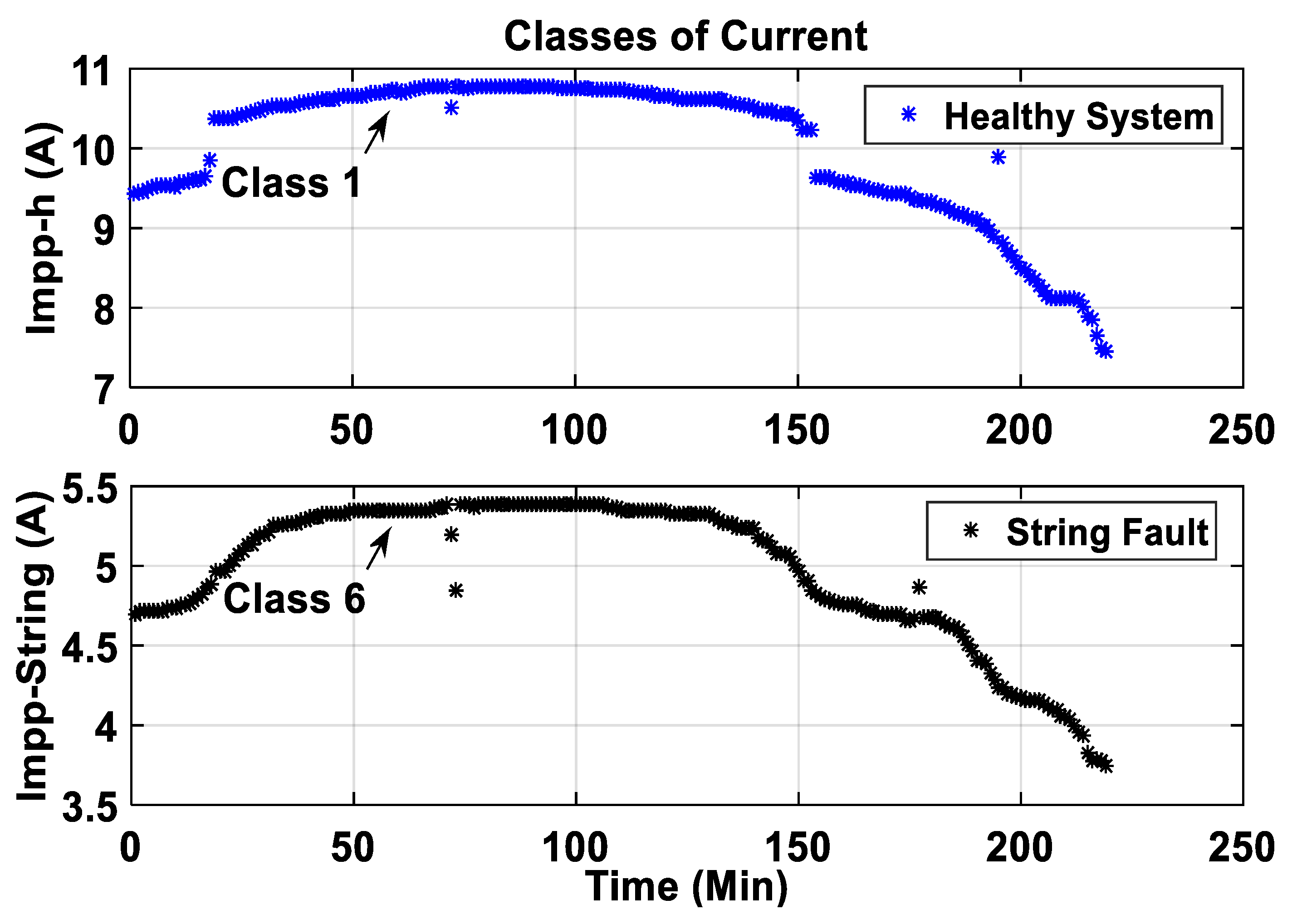
The two classes obtained from the NANN1 are shown in Figure 11. The classes are represented by graphs of the current values modeled at the maximum power point. These two classes for the MPP current are obtained from the NANN1 described in Figure 8.
- -
- The first graph (in blue line) represents Class 1, which models the MPP current at the healthy state.
- -
- The second graph (in black line) represents Class 6, which models the MPP current at a faulty state with a short-circuited string.
- -
- -
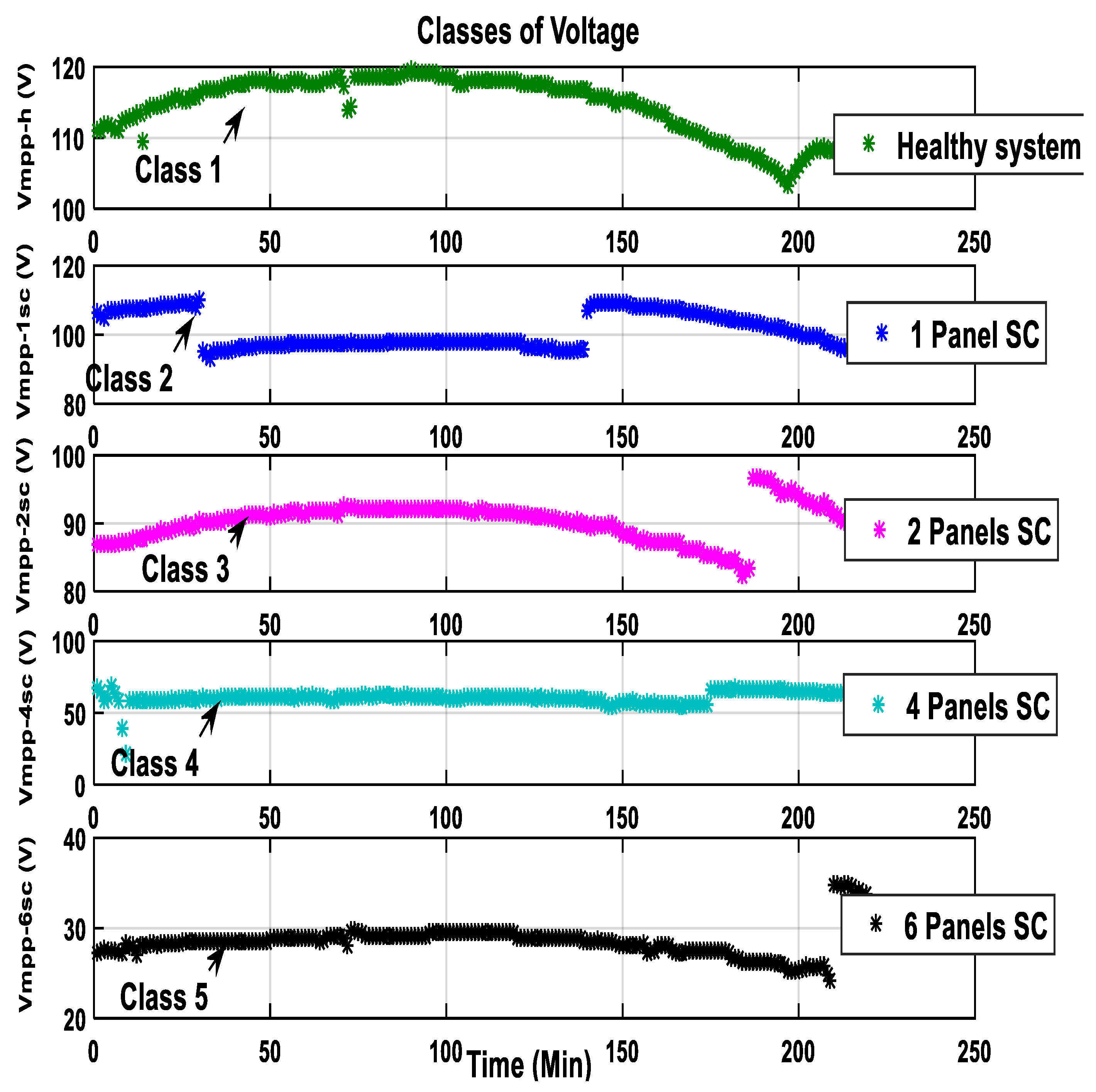
- The first graph (in green line) represents Class 1, which stands for the healthy voltage model at MPP.
- -
- The second graph (in blue line) represents Class 2, which stands for the faulty voltage model at MPP for one short-circuited panel.
- -
- The third graph (in magenta line) represents Class 3, which stands for the faulty voltage model at MPP for two short-circuited panels.
- -
- The fourth graph (in cyan line) represents Class 4, which stands for the faulty voltage model at MPP for four short-circuited panels.
- -
- The fifth graph (in black line) represents Class 5, which stands for the faulty voltage at MPP for six short-circuited panels.
Therefore, by combining the results from the two above figures, the following models occur:
- -
- -
- -
- The faulty model one short-circuited panel (Vmpp1sc with blue Figure 12).
- -
- The faulty model two short-circuited panels (Vmpp2sc with magenta Figure 12).
- -
- The faulty model four short-circuited panels (Vmpp4sc with cyan Figure 12).
- -
- The faulty model six short-circuited panels (Vmpp6sc with black Figure 12).
From this second step, six classes are defined, as presented in Table 5.
2.3. Diagnosis, Classification and Decision Using PNNs
The third step is diagnostic. It consists of injecting the outputs from the NANNs together with measured time variation of current and voltage from the solar panel array into two probabilistic neural networks, PNN1 and PNN2. The data to be injected are:
The fault detection algorithm compares the real measured data with output modeled from the NANNs. PNNs are used to diagnose healthy or faulty operation of solar PV panels. The main role of these PNNs is to classify, in real-time, the real measured currents and voltages according to models from NANN1 and NANN2. The analysis of the main characteristics of Impp and Vmpp of each output, along with measured data in real operating conditions, leads to the identification and isolation of failures.
The PNN is a monitored neural network widely used in pattern recognition; it has the potential for fault diagnosis and distributed parallel processing, self-organization, and self-learning. The following characteristics distinguish PNN from the other networks in the learning process [30]:
- ▪
- A PNN uses the probabilistic model, Bayesian classifiers.
- ▪
- A PNN is guaranteed to converge to a Bayesian classifier when enough training data are provided.
- ▪
- No learning process is required in PNNs.
- ▪
- No need to initialize the weights of the PNN.
- ▪
- There is no relationship between the learning and recall process.
The PNNs receive nine data points at a time (Figure 4), three for the PNN1 and six for the PNN2. The PNN1 will classify the current data into two classes, while the PNN2 will classify the voltage data into five classes. For each data vector, the PNN will work over a range of at least 220 data points by using data in memory. The final decision will be taken in the last step as explained in the following Table 6.
• Obtained classification
We consider one healthy operation and five types of faults, one for the current and four for the voltage. First, the outputs from PNN1 illustrated in Figure 13 show the classification for current fault (Class 6) at Impp. It shows that a string fault directly impacts the output current of the PV array.
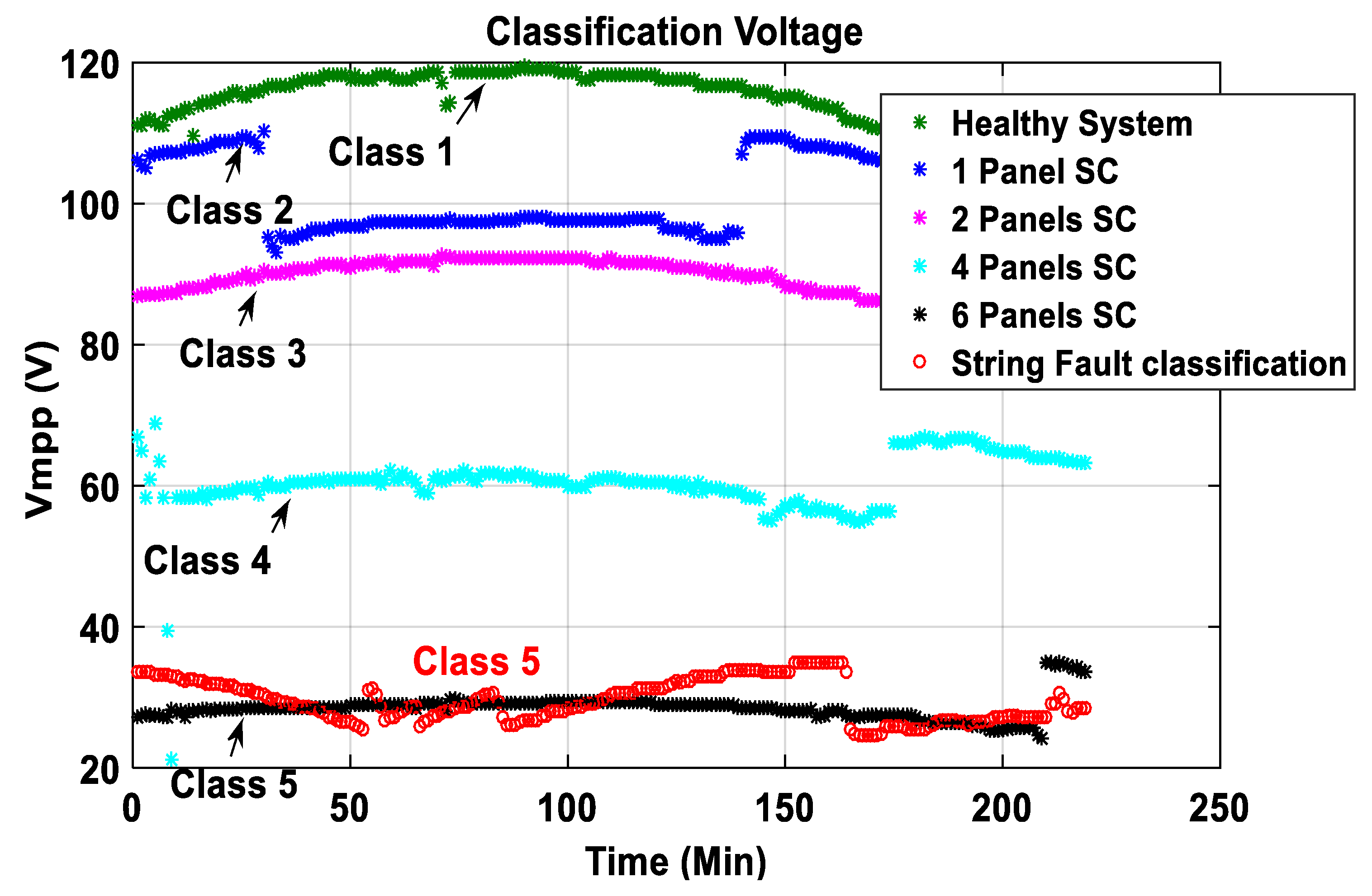
Then, the outputs from the PNN2 illustrated in Figure 14 show the classification for the four voltage faults (Classes 2–5) in Vmpp.
The PNNs classifies the real current and voltage data input using the Classes shown in Figure 13 and Figure 14.
In Figure 13, we present a graph, in red, representing the current at MPP classified as Class 6 (see also Table 5). Additionally, in Figure 14, the red color graph represents the voltage at MPP classified as Class 5 (Table 5).
In this third diagnosis stage, a routine collects decisions from both PNNs following Table 6 and thus calculates the probability density function (PDF) [36].
Unlike multi-layer perceptron (MLP) networks, radial basis (RBF) functions (including PNNs) use radial functions instead of sigmoidal activation functions. They build a local decision function centered at a subset of the input space [37]. The global decision function is the sum of all local functions [30,38].
In the context of pattern classification, every observed vector ( is a -dimensional vector) is placed inside one of the predefined cluster classes:
where is the number of possible classes that x can belong to ( = six in this study).
The classifier’s efficiency is limited by the length of the input vector and the number of possible classes .
The Bayes classifier uses the Bayes conditional probability rule that is the probability for x to belong to a class .
This probability is given by:
where:
- is the conditional probability density function of x given .
- is the probability of choosing a sample from the class .
An input vector x is classified to belong to the class, if:
The estimation process of the later probabilities from a learning set uses Parzen’s windowing technique to determine the PDF [30,36]. Therefore, the estimator used for the PNN networks,, is given by:
where represents the sample belonging to the class and is a smoothing parameter.
When the diagnosis algorithm is executed, it will display the errors and decide about the state of the system, as shown in Figure 15.
All three steps (data feeding, faults modeling, and decision about diagnosis) should be reiterated at each classification.
3. Details about the Elaboration of NANNS
This section presents more details for modeling the ANNs used in NANNs. The approach given may work well for a whole life cycle of the PV system but requires substantial prior work, which includes:
- -
- The collection of real measured data (T, G, Impp, Vmpp), reserved for learning and validating NANNs.
- -
- The choice of the type of ANNs (multi-layer perceptron (MLP)) and their architectures.
- -
- The choice of the learning type (supervised learning).
- -
- The validation of NANNs.
- -
- The exploitation of the results.
In what follows, we provide more details about each of these steps.
3.1. Collection of Real Measured Data
The data from the station at the CDER, including panels’ temperature, solar irradiance, PV current, and PV voltage, were collected on 20 March 2018, for a period of about 460 data points, as presented in Figure 16.
3.2. Choice of Type of ANNs and Their Architectures
The developed ANNs are based on a multi-layer perceptron (MLP). Several simulations were carried out, varying the number of hidden layers and neurons in each hidden layer to find the optimal network architecture. Table 3 and Table 4 summarize the final architectures of each ANN.
The inputs to the ANNs are the temperature and irradiance. Simultaneously, the outputs are Impp (supervised following real healthy and real faulty) and Vmpp (supervised following real healthy and real faulty) as described in Figure 17. Besides, faults are introduced in the real PV system to obtain real current and voltage data for each faulty mode.
3.3. Choice of Learning Type
The weights adjustment uses the Levenberg–Marquardt (LM) [39] backpropagation algorithm available in Matlab 2015a Software environment. Results after learning from a healthy ANN are summarized in Figure 20 below, which shows good training performance.
The appropriate neural structure is characterized by the transfer function of a hyperbolic tangent in the first hidden layer (for ANNS) and a linear transfer function in the second hidden layer (for PNNs).
Regression of complex training process of NNs based controllers is shown in the following Figure 21.
Figure 21 illustrates that the major scatter (Target output) points are regrouped around the right (Y = T), which demonstrates the good efficiency of the approach.
3.4. Validation of ANNs
The remaining data points out of 460 from Figure 16 are used for validation. In what follow, some cases for healthy and faulty scenarios are presented.
• Healthy system validation
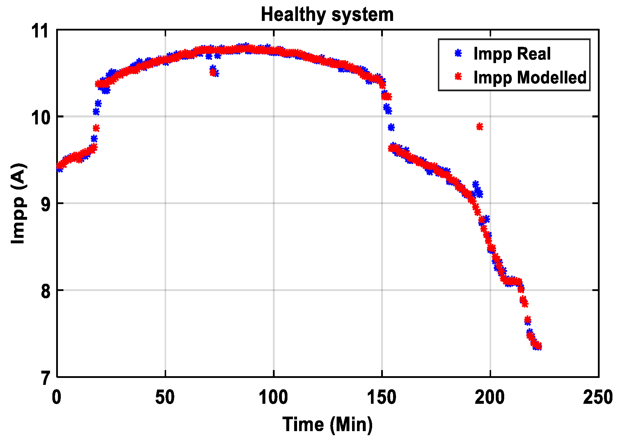
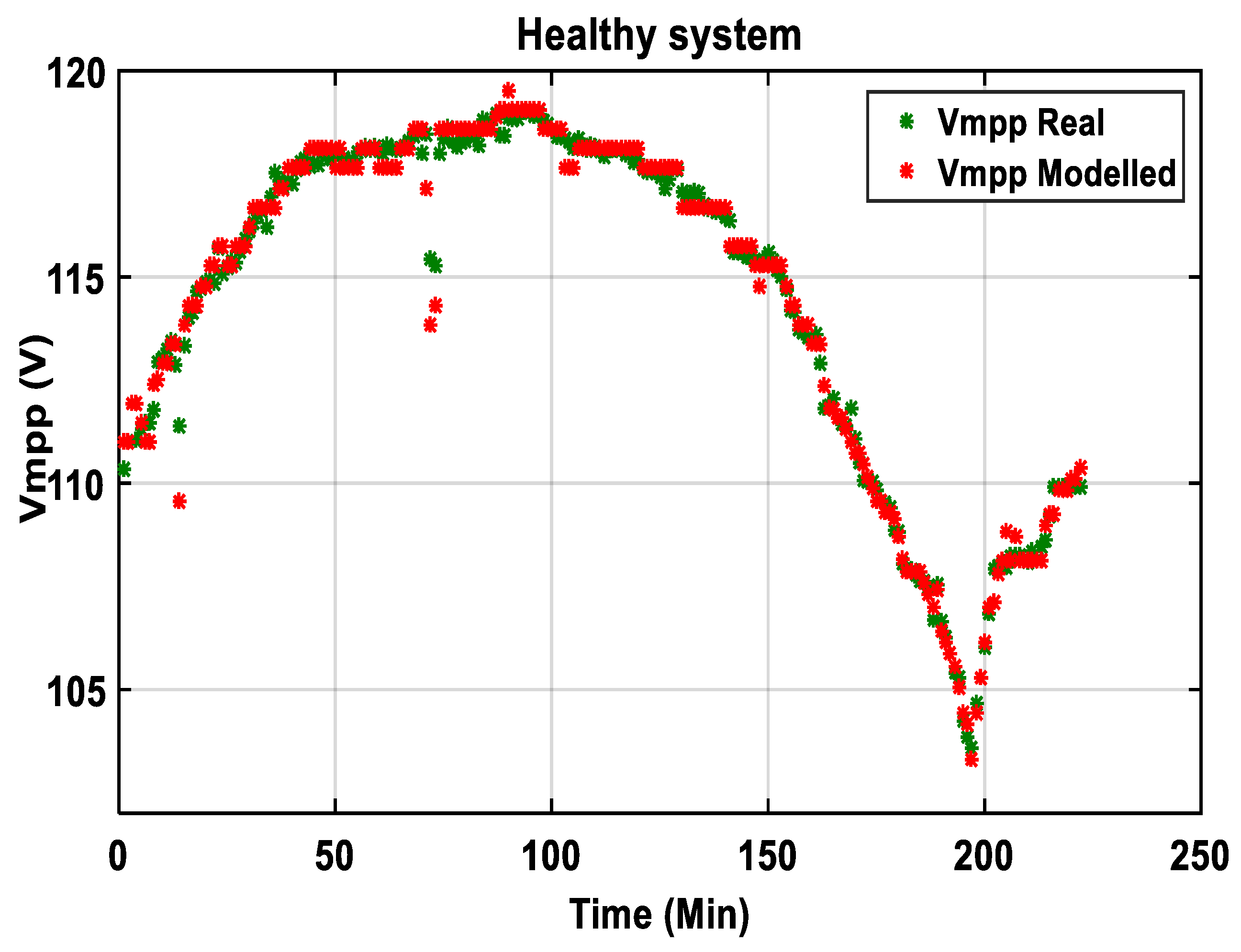
Modeling by ANNs, as shown in Figure 22 and Figure 24, shows a high fitting between the real data (current and voltage) and the ones estimated by the modeled ANNs in a healthy system.
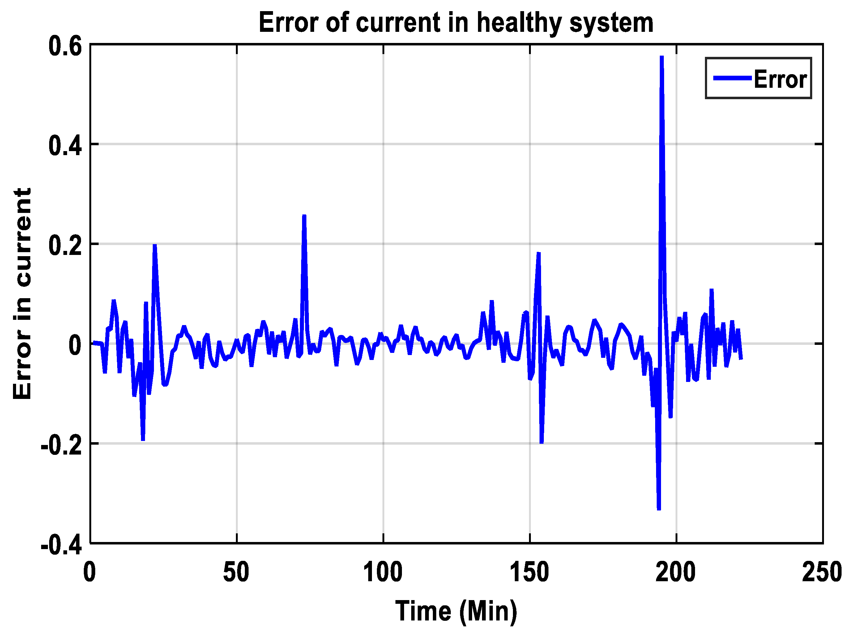
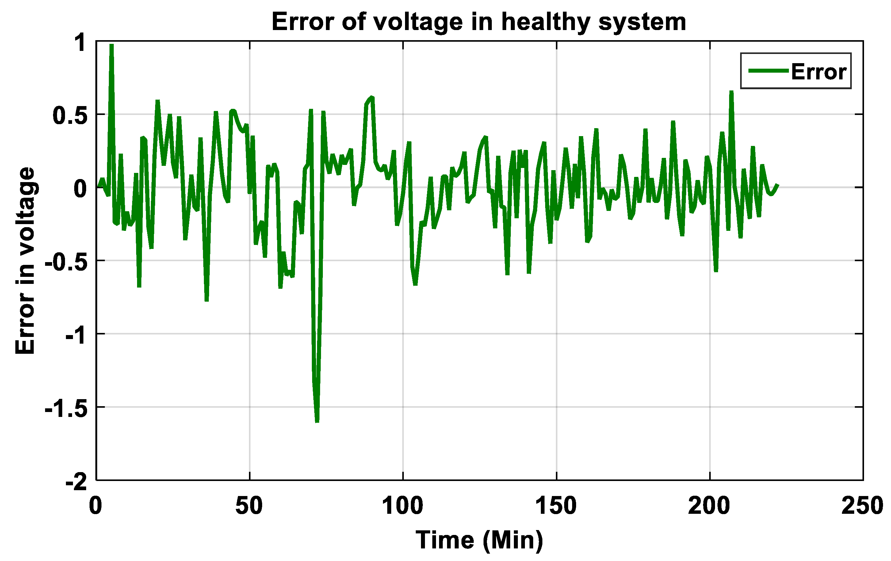
The error between real and modeled voltage data for a healthy system is depicted in Figure 25 below.
It can be seen from the reduced values of errors in Figure 23 and Figure 25 that there is a good agreement between modeled and real data, which indicates the good performance of the developed NANN1-model and NANN2-model. Therefore, the network weights and bias of the network are well adjusted, and the model can reproduce the output data with good accuracy.
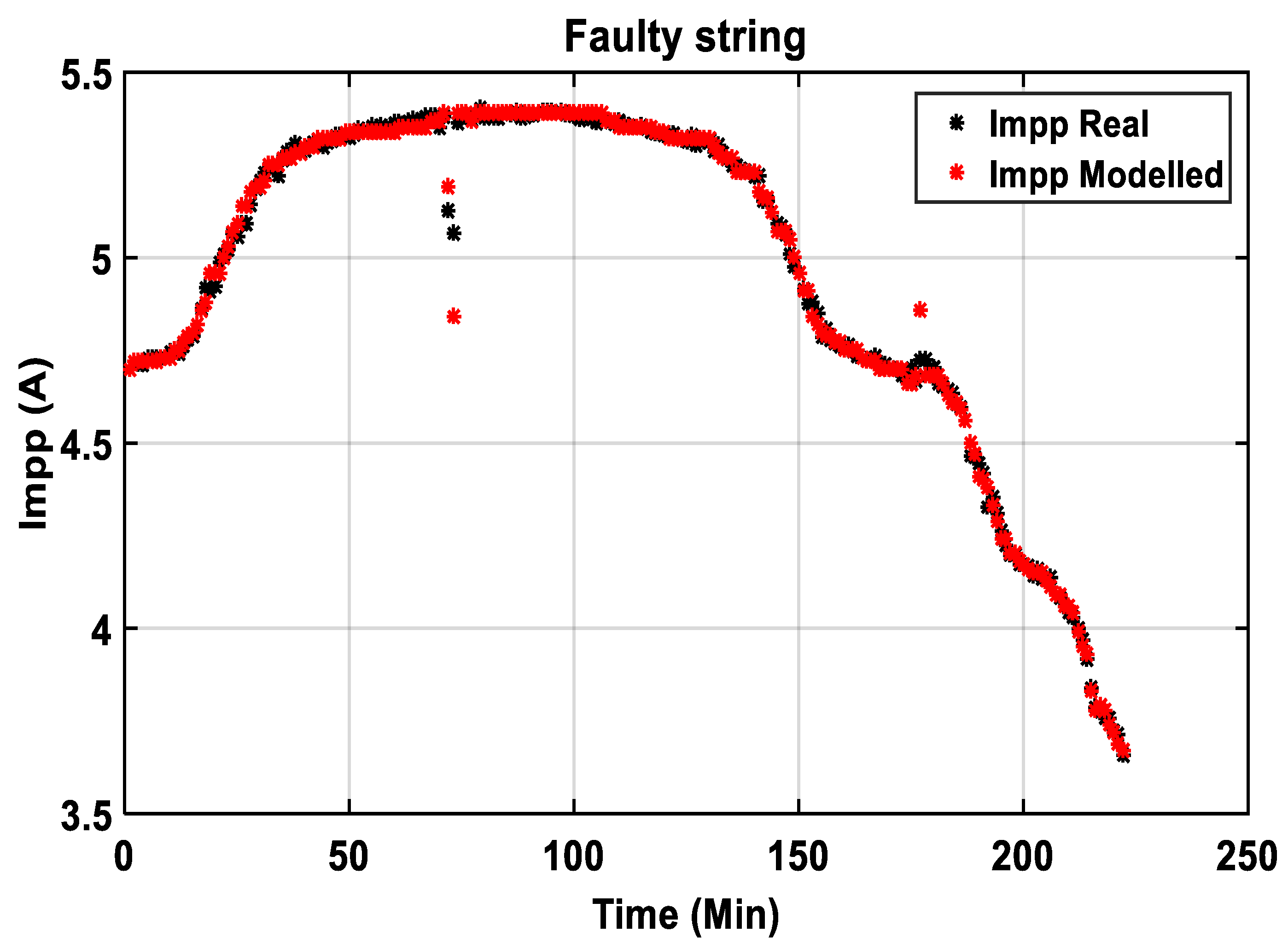
• Faulty system validation
3.5. Exploitation of Results
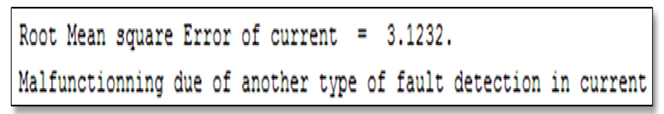
The diagnosis step of the PV plant, using the classification method, consists of using the root mean square error (RMSE) and the mean relative error (MRE) methods to display the state of the PV array. For example, for a faulty PV plant, Figure 28 and Figure 29 show the state of faulty current and voltage, respectively.
The expression of root mean squared error (RMSE) is:
where:
- N: number of data points.
The equation of the relative mean error (MRE) is as follows:
where:
- DataMean: Mean of real data points.
The relative mean error has no unit; it tells us the quality (accuracy) of the results of obtained voltage. It is usually expressed in percentage (%).
Additional results of obtained errors (RMSE, MRE) for each class of the real PV array are presented in Table 7 below.
4. Test of Robustness
The robustness of the ANNs based fault diagnosis method is assessed by introducing noises in the PV plant and showing the effect on injected data. Moreover, noise can be perceived as an error, a statistical uncertainty or an undesired random disturbance of a useful modeled response of the PV array. Several different effects can cause such noise, such as thermal noise, device type, or manufacturing quality.
4.1. Presence of Noise from the Inverter
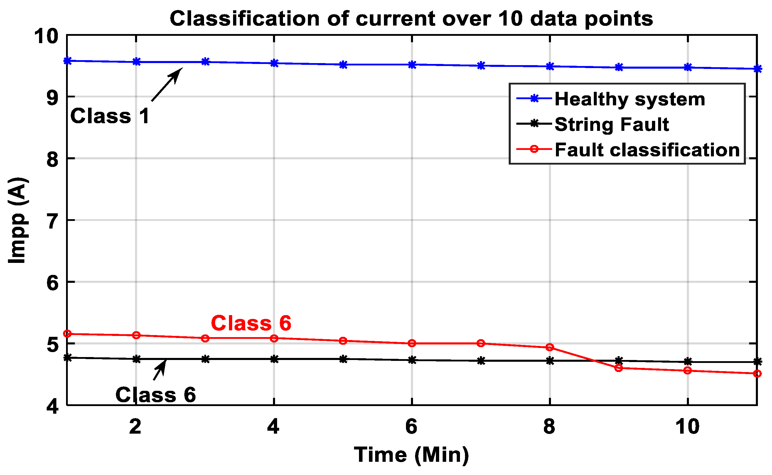
In PV plants, faults usually occur from the electrical grid (instability) or the storage system. Most widespread are from inverters or the photovoltaic array. Therefore, the inverter can cause major perturbations if damaged or faulted. In this subsection, the PV plant is connected to the grid through an inverter. We artificially added inverter-generated noise in the current and voltage vectors to be classified. Figure 30 and Figure 31 show the classification of the overall system (current and voltage) along with the results from the faulty string model in the presence of noise from the inverter. In Figure 30, we observe that the inputs are noised by the large space between the real current (Class 1) in blue and the classified one in red.
Figure 30 illustrates that the classification of current (in red) is closer to the healthy current (in blue) than the defective current (in black). The most important data belong to class 1 (for a healthy system).
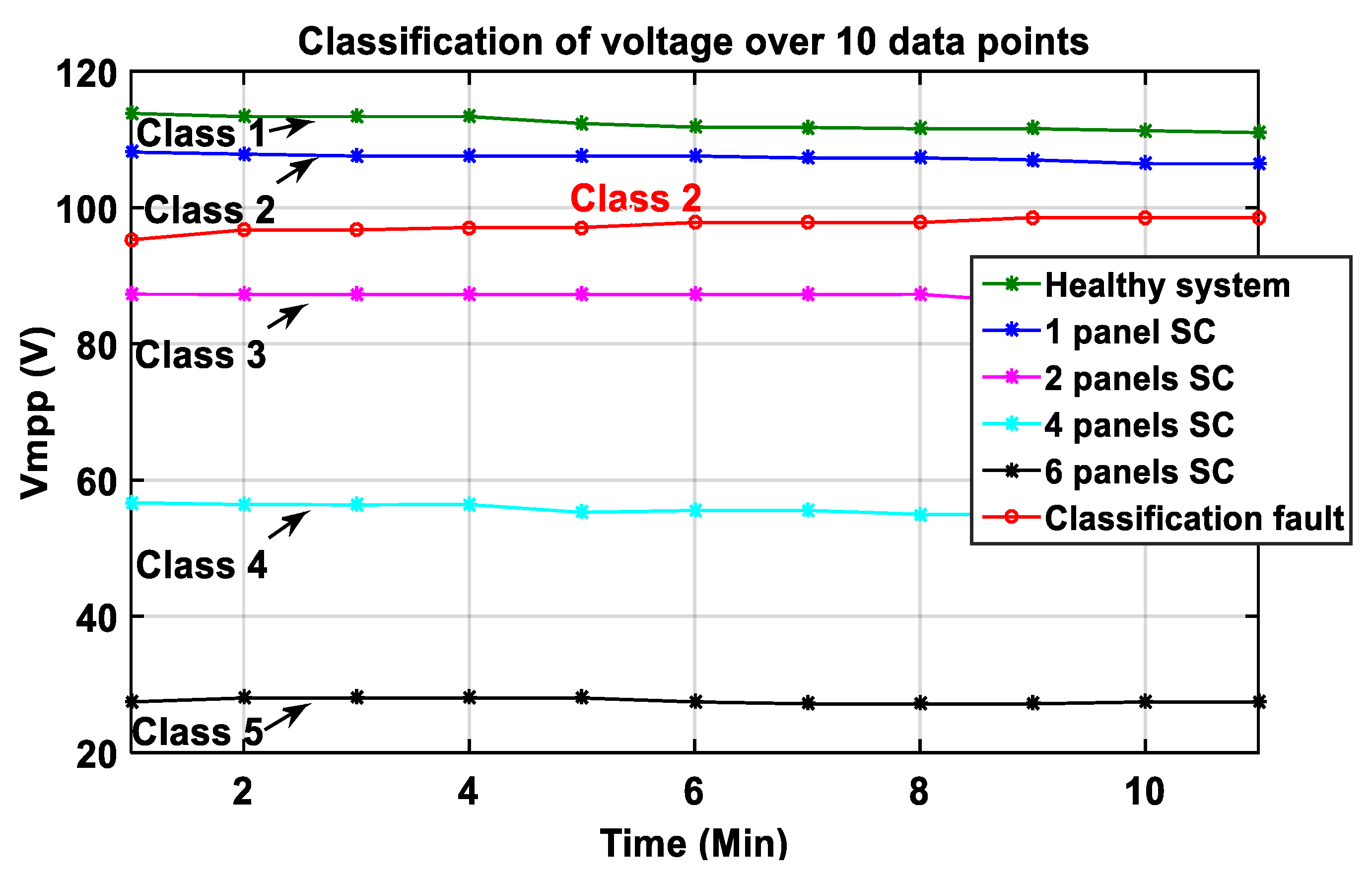
Figure 31 shows that the classification of the voltage (in red) is closer to the healthy voltage (in green) than the other defective voltages (in blue, magenta, cyan, and black). Besides, even though the data to be classified is corrupted by noise from the inverter, the proposed approach was able to classify it correctly (Figure 30 and Figure 31), which shows the effectiveness of PNNs classification.
4.2. Effect of Detection Time
5. Conclusions
Automatic monitoring, detection, and diagnosis of faults that occur in photovoltaic plants/arrays have recently become a very important research topic. In this paper, an efficient neural network-based method was developed to diagnose several failure scenarios that may occur in a photovoltaic array at short circuits. The model used for the simulation of healthy and defectives conditions was experimentally validated by real data from a photovoltaic array installed at the CDER station in Algiers, Algeria. The developed method was elaborated in three main steps: feeding experimental data to the neural networks, modeling faults using NANNs and decision about diagnosis using PNNs. Each fault was detected and classified. The obtained results confirm the effectiveness of the developed models to locate and identify different types of failures even with noises. The proposed fault diagnosis method can easily be generalized and applied to large-scale PV plants. Besides, the developed method is straightforward and requires only the following parameters: the array’s temperature, solar irradiance, PV voltage, and PV current of the PV array (time variation). In the proposed study, seven ANNs and two PNNs were required, necessitating a different treatment for currents and voltages because rough estimation is slightly different. In perspective, we plan to carry on the work considering only a single parameter such as power through online adaptation. Besides, the decision on the system’s quality is made at every single data point, and it is possible to use previous data scrolling in real-time.
Author Contributions
Conceptualization, S.T.K.; methodology, N.C.; writing—original draft preparation, S.T.K.; writing—review and editing, S.B. and A.I.; visualization, S.B.; supervision, N.C.; project administration, A.I. All authors have read and agreed to the published version of the manuscript.
Funding
This research received no external funding.
Institutional Review Board Statement
The study was conducted according to the guidelines of the Declarations of Helsinki, and approved the Institutional Review Board.
Informed Consent Statement
Informed consent was obtained from all subjects involved in the study.
Conflicts of Interest
The authors declare no conflict of interest.
Nomenclature
| PV | Photovoltaic |
| BBD | Blocking and bypassing diode |
| OC | Open circuit |
| SC | Short circuit |
| GF | Ground fault |
| LLF | Line-to-line |
| AF | Arc fault |
| FDD | Fault detection and diagnosis |
| IR | Infrared |
| AI | Artificial intelligence |
| ANN | Artificial neural network |
| MLP | Multi-layer perceptron |
| RBN | Radial basis network |
| FF | Feed-forward |
| RNN | Recurrent neural network |
| NN | Neural network |
| MPP | Maximum power point |
| ANNs | Artificial neural networks |
| NANNs | Networks of artificial neural networks |
| NANN1 | Network of artificial neural network 1 |
| NANN2 | Network of artificial neural network 2 |
| PNNs | Probabilistic neural networks |
| I-V | Current–voltage curve |
| CDER | Renewable Energies Development Centre |
| G | Solar irradiance |
| T | Panel’s temperature |
| Pmpp | Maximum power |
| Isc | Short circuit current |
| Voc | Open circuit voltage |
| α | Coefficient of temperature at Isc |
| β | Coefficient of temperature at Voc |
| Impp | Maximum current |
| Vmpp | Maximum voltage |
| Impp_h | Healthy current at the maximal power point |
| Vmpp_h | Healthy voltage at the maximal power point |
| Vmpp1sc | Voltage at maximum power point of one short-circuited panel |
| Vmpp2sc | Voltage at maximum power point of two short-circuited panels |
| Vmpp4sc | Voltage at maximum power point of four short-circuited panels |
| Vmpp6sc | Voltage at maximum power point of six short-circuited panels |
| Impp_s | Current at maximal power point of string fault |
| Probability density function | |
| RBF | Radial basis functions |
| LM | Levenberg–Marquardt |
| RMSE | Root mean square error |
| MRE | Mean relative error |
References
- Hu, Y.; Cao, W. Theoretical Analysis and Implementation of Photovoltaic Fault Diagnosis. In Renewable Energy—Utilisation and System Integration; IntechOpen: London, UK, 2016. [Google Scholar]
- Alam, M.K.; Khan, F.; Johnson, J.; Flicker, J. A Comprehensive Review of Catastrophic Faults in PV Arrays: Types, Detection, and Mitigation Techniques. IEEE J. Photovolt. 2015, 5, 982–997. [Google Scholar]
- Branco, G.; Costa, A. Tailored Algorithms for Anomaly Detection in Photovoltaic Systems. Energies 2020, 13, 225. [Google Scholar] [CrossRef] [Green Version]
- Quintana, M.A.; King, D.L.; McMahon, T.J.; Osterwald, C.R. Commonly observed degradation in field-aged photovoltaic modules. In Proceedings of the Conference Record of the Twenty-Ninth IEEE Photovoltaic Specialists Conference, New Orleans, LA, USA, 19–24 May 2002; pp. 1436–1439. [Google Scholar]
- Deline, C. Partially shaded operation of multi-string photovoltaic systems. In Proceedings of the 35th IEEE Photovoltaic Specialists Conference, Honolulu, HI, USA, 20–25 June 2010; pp. 394–399. [Google Scholar]
- Silverman, T.J.; Deceglie, M.G.; Subedi, I.; Podraza, N.J.; Slauch, I.M.; Ferry, V.E. Reducing Operating Temperature in Photovoltaic Modules. IEEE J. Photovolt. 2018, 8, 532–540. [Google Scholar] [CrossRef]
- Koentges, M.; Kurtz, S.; Packard, C.E.; Jahn, U.; Berger, K.A.; Kato, K.; Friesen, T.; Liu, H.; Van Iseghem, M.; Wohlgemuth, J.; et al. Review of Failures of Photovoltaic Modules. 2014. Available online: https://www.researchgate.net/publication/274717701_Review_of_Failures_of_Photovoltaic_Modules (accessed on 20 April 2021).
- Coello, M.; Boyle, L. Simple Model for Predicting Time Series Soiling of Photovoltaic Panels. IEEE J. Photovolt. 2019, 9, 1382–1387. [Google Scholar] [CrossRef]
- Lindig, S.; Kaaya, I.; Weiss, K.; Moser, D.; Topic, M. Review of Statistical and Analytical Degradation Models for Photovoltaic Modules and Systems as Well as Related Improvements. IEEE J. Photovolt. 2018, 8, 1773–1786. [Google Scholar] [CrossRef]
- Laukamp, H.; Schoen, T.; Ruoss, D. Reliability Study of Grid Connected PV Systems. Field Exp. Recomm. Des. Pract. 2002, 31. Available online: https://iea-pvps.org/wp-content/uploads/2020/01/rep7_08.pdf (accessed on 20 April 2021).
- Heinrich Haeberlin, J.D.; Berner Fachhochschule, G. Gradual Reduction of PV Generator Yield due to Pollution. In Proceedings of the 2nd World Conference on Photovoltaic Solar Energy Conversion, Vienna, Austria, 6–10 July 1998. [Google Scholar]
- Mellit, A.; Tina, G.M.; Kalogirou, S.A. Fault detection and diagnosis methods for photovoltaic systems: A review. Renew. Sustain. Energy Rev. 2018, 91, 1–17. [Google Scholar] [CrossRef]
- Pillai, D.S.; Rajasekar, N. A comprehensive review on protection challenges and fault diagnosis in PV systems. Renew. Sustain. Energy Rev. 2018, 91, 18–40. [Google Scholar] [CrossRef]
- Meyer, E.L.; Dyk, E.E. Assessing the reliability and degradation of photovoltaic module performance parameters. IEEE Trans. Reliab. 2004, 53, 83–92. [Google Scholar] [CrossRef]
- Jones, R.K.; Baras, A.; Saeeri, A.; Qahtani, A.A.; Amoudi AO, A.; Shaya, Y.A. Optimized Cleaning Cost and Schedule Based on Observed Soiling Conditions for Photovoltaic Plants in Central Saudi Arabia. IEEE J. Photovolt. 2016, 6, 730–738. [Google Scholar] [CrossRef]
- Guerriero, P.; Daliento, S. Toward a Hot Spot Free PV Module. IEEE J. Photovolt. 2019, 9, 796–802. [Google Scholar] [CrossRef]
- Woyte, A.; Nijs, J.; Belmans, R. Partial shadowing of photovoltaic arrays with different system configurations: Literature review and field-test results. Sol. Energy 2003, 74, 217–233. [Google Scholar] [CrossRef]
- King, D.; Quintana, M.; Kratochvil, J.; Ellibee, D.; Hansen, B. Photovoltaic module performance and durability following long-term field exposure. Prog. Photovolt. Res. Appl. 2000, 8, 241–256. [Google Scholar] [CrossRef] [Green Version]
- Munoz, M.A.; Alonso-García, M.C.; Vela, N.; Chenlo, F. Early degradation of silicon PV modules and guaranty conditions. Sol. Energy 2011, 85, 2264–2274. [Google Scholar] [CrossRef]
- Pierdicca, R.; Malinverni, E.; Piccinini, F.; Paolanti, M.; Felicetti, A.; Zingaretti, P. Deep convolutional neural network for automatic detection of damaged photovoltaic cells. Int. Arch. Photogramm. Remote Sens. Spatial Inf. Sci. 2018, XLII-2, 893–900. [Google Scholar] [CrossRef] [Green Version]
- Haque, A.; Kurukuru VS, B.; Khan, M.; Khan, I.; Jaffery, Z. Fault diagnosis of Photovoltaic Modules. Energy Sci. Eng. 2019, 7, 622–644. [Google Scholar] [CrossRef] [Green Version]
- Platon, R.; Martel, J.; Woodruff, N.; Chau, T.Y. Online Fault Detection in PV Systems. IEEE Trans. Sustain. Energy 2015, 6, 1200–1207. [Google Scholar] [CrossRef]
- Appiah, A.Y.; Zhang, X.; Ayawli BB, K.; Kyeremeh, F. Review and Performance Evaluation of Photovoltaic Array Fault Detection and Diagnosis Techniques. Int. J. Photoenergy 2019, 2019, 19. [Google Scholar] [CrossRef]
- Chouder, A. Analysis, Diagnosis and Fault Detection in Photovoltaic Systems. Ph.D. Thesis, Universitat Politècnica de Catalunya, Barcelona, Spain, 2010. [Google Scholar]
- Mellit, A.; Kalogirou, S.A. Artificial intelligence techniques for photovoltaic applications: A review. Prog. Energy Combust. Sci. 2008, 34, 574–632. [Google Scholar] [CrossRef]
- Chine, W.; Mellit, A.; Lughi, V.; Malek, A.; Sulligoi, G.; Massi Pavan, A. A novel fault diagnosis technique for photovoltaic systems based on artificial neural networks. Renew. Energy 2016, 90, 501–512. [Google Scholar] [CrossRef]
- Yuchuan, W.; Qinli, L.; Yaqin, S. Application of BP neural network fault diagnosis in solar photovoltaic system. In Proceedings of the 2009 International Conference on Mechatronics and Automation, Changchun, China, 9–12 August 2009; pp. 2581–2585. [Google Scholar]
- Hwang, H.-R.; Kim, B.-S.; Cho, T.-H.; Lee, I.-S. Implementation of a Fault Diagnosis System Using Neural Networks for Solar Panel. Int. J. ControlAutom. Syst. 2019, 17, 1050–1058. [Google Scholar] [CrossRef]
- Syafaruddin Karatepe, E.; Hiyama, T. Controlling of artificial neural network for fault diagnosis of photovoltaic array. In Proceedings of the 2011 16th International Conference on Intelligent System Applications to Power Systems, Hersonissos, Greece, 25–28 September 2011; pp. 1–6. [Google Scholar]
- Specht, D.F. Probabilistic neural networks. Neural Netw. 1990, 3, 109–118. [Google Scholar] [CrossRef]
- Yu, Y.; Sheng, D.; Chen, J. A novel sensor fault diagnosis method based on Modified Ensemble Empirical Mode Decomposition and Probabilistic Neural Network. Measurement 2015, 68, 328–336. [Google Scholar] [CrossRef]
- Lin, F.J.; Lu, S.Y.; Chao, J.Y.; Chang, J.K. Intelligent PV Power Smoothing Control Using Probabilistic Fuzzy Neural Network with Asymmetric Membership Function. Int. J. Photo Energy 2017, 2017, 15. [Google Scholar] [CrossRef] [Green Version]
- Chouder, A.; Silvestre, S. Automatic supervision and fault detection of PV systems based on power losses analysis. Energy Convers. Manag. 2010, 51, 1929–1937. [Google Scholar] [CrossRef]
- Chouder, A.; Silvestre, S.; Taghezouit, B.; Karatepe, E. Monitoring, modelling and simulation of PV systems using LabVIEW. Solar Energy 2013, 91, 337–349. [Google Scholar] [CrossRef]
- Sobhani-Tehrani, E.; Khorasani, K. Fault Diagnosis of Nonlinear Systems Using a Hybrid Approach; Springer: Berlin/Heidelberg, Germany, 2009. [Google Scholar]
- Parzen, E. On Estimation of a Probability Density Function and Mode. Ann. Math. Stat. 1962, 33, 1065–1076. [Google Scholar] [CrossRef]
- Burrascano, P. Learning vector quantization for the probabilistic neural network. IEEE Trans. Neural Netw. 1991, 2, 458–461. [Google Scholar] [CrossRef] [PubMed]
- Kim, M.W.; Arozullah, M. Generalized probabilistic neural network based classifiers. In Proceedings of the IJCNN International Joint Conference on Neural Networks, Baltimore, MD, USA, 7–11 June 1992; Volume 3, pp. 648–653. [Google Scholar]
- Dkhichi, F.; Oukarfi, B.; Fakkar, A.; Belbounaguia, N. Parameter identification of solar cell model using Levenberg–Marquardt algorithm combined with simulated annealing. Sol. Energy 2014, 110, 781–788. [Google Scholar] [CrossRef]
Figure 1.
Causes of failures in PV systems.

Figure 2.
Major causes of failures in PV array.

Figure 3.
Global structure of the monitored PV plant for fault detection and diagnosis.

Figure 4.
Exploitation process of diagnosis in the PV array.

Figure 5.
Global organigram of developing functioning of PV diagnosis process.

Figure 6.
Real data of (a) array’s temperature; (b) solar irradiance; (c) PV current; (d) PV voltage.
Figure 6.
Real data of (a) array’s temperature; (b) solar irradiance; (c) PV current; (d) PV voltage.

Figure 7.
A generic neural network-based multiple-model fault detection and isolation scheme [36].
Figure 7.
A generic neural network-based multiple-model fault detection and isolation scheme [36].

Figure 8.
The current modeling structure by a network of artificial neural networks (NANN1).

Figure 9.
The voltage modeling structure by a network of artificial neural networks (NANN2).

Figure 10.
Classes obtained for the current/voltage modeled at MPP.

Figure 11.
Classes obtained for the current modeled at MPP.

Figure 12.
Classes obtained for voltage modeled at MPP.

Figure 13.
Classification of the current fault at the maximum power point.

Figure 14.
Classification of voltage faults at the maximum power point.

Figure 15.
Snapshot of the classification result and estimation errors about the PV system.

Figure 16.
Collected meteorological and electrical data for 460 data points.

Figure 17.
Process of supervising and weight adjustments in ANN1 for a healthy system.

Figure 18.
Data provided to the ANN1 from NANN1 in a healthy system for the current learning process.
Figure 18.
Data provided to the ANN1 from NANN1 in a healthy system for the current learning process.

Figure 19.
Data provided to the ANN1 from NANN2 in a healthy system for the voltage learning process.
Figure 19.
Data provided to the ANN1 from NANN2 in a healthy system for the voltage learning process.

Figure 20.
Generated toolbox interface for the developed NNs training on Matlab.

Figure 21.
Generated regression of training process.

Figure 22.
Real vs. modeled data from current, Impp in a healthy system.

Figure 23.
The error between Impp-Real and Impp-Modelled.

Figure 24.
Real and modeled data from voltage, Vmpp in a healthy system.

Figure 25.
The error between Vmpp-Real and Vmpp-modelled.

Figure 26.
Real and modeled data from current, Impp in a faulty string system.

Figure 27.
Real and modeled data from voltage, Vmpp in a faulty system (1 Panel SC).

Figure 28.
RMSE command window results for a fault at current.

Figure 29.
MRE command window results for fault at six panels SC.

Figure 30.
Classification of current at maximum power point in the presence of noise from the inverter.
Figure 30.
Classification of current at maximum power point in the presence of noise from the inverter.

Figure 31.
Classification of voltage at maximum power point in the presence of noise from the inverter.
Figure 31.
Classification of voltage at maximum power point in the presence of noise from the inverter.

Figure 32.
Classification of current at maximum power point in the presence of noise from an inverter, over 10 data points.
Figure 32.
Classification of current at maximum power point in the presence of noise from an inverter, over 10 data points.

Figure 33.
Classification of voltage at maximum power point in the presence of noise from the inverter, over 10 data points.
Figure 33.
Classification of voltage at maximum power point in the presence of noise from the inverter, over 10 data points.


Table 1.
The Isofoton 106-12 specifications.
| Parameters | Values |
|---|---|
| Maximum power (Pmpp) | 106 W |
| Short circuit current (Isc) | 6.54 A |
| Open circuit voltage (Voc) | 21.6 V |
| Coefficient of temperature at Isc (α) | 0.060 %/°C |
| Coefficient of temperature at Voc (β) | −0.36 %/°C |
| Maximum current (Impp) | 6.1 A |
| Maximum voltage (Vmpp) | 17.4 V |
Table 2.
Type of faults and their symbols in the PV array.
| Name of Faults | Symbols |
|---|---|
| Healthy model | C1 |
| Fault detection due to voltage of one short-circuited panel | C2 |
| Fault detection due to voltage of two short-circuited panels | C3 |
| Fault detection due to voltage of four short-circuited panels | C4 |
| Fault detection due to voltage of six short-circuited panels | C5 |
| Fault detection due to current of short-circuited string | C6 |
Table 3.
The architecture of the two ANNs developed in NANN1.
| Numbers | ANNs of NANN1 | Input Layer | Hidden Layer | Output Layer |
|---|---|---|---|---|
| ANN1 | Healthy current | 2 | 40 | 1 (Impp_healthy) |
| ANN2 | Fault in the current of string short circuited | 2 | 40 | 1 (Impp_string) |
Table 4.
The architecture of the five ANNs developed in NANN2.
| Numbers | ANNs of NANN2 | Input Layer | Hidden Layer | Output Layer |
|---|---|---|---|---|
| ANN1 | Healthy voltage model | 2 | 40 | 1 (Vmpp_healthy) |
| ANN2 | Fault in voltage of one panel SC | 2 | 40 | 1 (Vmpp_1SC) |
| ANN3 | Fault in voltage of two panels SC | 2 | 40 | 1 (Vmpp_2SC) |
| ANN4 | Fault in voltage of four panels SC | 2 | 40 | 1 (Vmpp_4SC) |
| ANN5 | Fault in voltage of six panels SC | 2 | 40 | 1 (Vmpp_6SC) |
Table 5.
Type of parameters with symbols and classes.
| Symbols | Parameters | Classes |
|---|---|---|
| Impp_h | Healthy current at the maximal power point | Class 1 |
| Vmpp_h | Healthy voltage at the maximal power point | Class 1 |
| Vmpp1sc | Voltage at maximum power point of one short-circuited panel | Class 2 |
| Vmpp2sc | Voltage at maximum power point of two short-circuited panels | Class 3 |
| Vmpp4sc | Voltage at maximum power point of four short-circuited panels | Class 4 |
| Vmpp6sc | Voltage at maximum power point of six short-circuited panels | Class 5 |
| Impp_s | Current at maximal power point of string fault | Class 6 |
Table 6.
Diagnosis and decision of the PV system.
| Impp | Vmpp | Decision about PV System |
|---|---|---|
| Impph | Vmpph | 2Healthy system |
| Impph | Vmpp1sc | Fault detection due to one short-circuited panel |
| Impph | Vmpp2sc | Fault detection due to two short-circuited panels |
| Impph | Vmpp4sc | Fault detection due to four short-circuited panels |
| Impph | Vmpp6sc | Fault detection due to six short-circuited panels |
| Imppstring | Vmpph | Fault detection due to string |
Table 7.
RMSE (root mean square error) and MRE (mean relative error (%)).
| Current Healthy System | Current String Fault | Voltage Healthy System | Voltage 1 Panel SC | Voltage 2 Panels SC | Voltage 4 Panels SC | Voltage 6 Panels SC | |
|---|---|---|---|---|---|---|---|
| RMSE | 0.5737 | 0.8264 | 2.4928 | 2.4493 | 1.1601 | 1.7280 | 0.8201 |
| MRE (%) | 3.21 | 1.62 | 1.78 | 1.02 | 1.51 | 1.54 | 1.67 |
Publisher’s Note: MDPI stays neutral with regard to jurisdictional claims in published maps and institutional affiliations. |
© 2021 by the authors. Licensee MDPI, Basel, Switzerland. This article is an open access article distributed under the terms and conditions of the Creative Commons Attribution (CC BY) license (https://creativecommons.org/licenses/by/4.0/).
Share and Cite
MDPI and ACS Style
Tchoketch Kebir, S.; Cheggaga, N.; Ilinca, A.; Boulouma, S. An Efficient Neural Network-Based Method for Diagnosing Faults of PV Array. Sustainability 2021, 13, 6194. https://0-doi-org.brum.beds.ac.uk/10.3390/su13116194
AMA Style
Tchoketch Kebir S, Cheggaga N, Ilinca A, Boulouma S. An Efficient Neural Network-Based Method for Diagnosing Faults of PV Array. Sustainability. 2021; 13(11):6194. https://0-doi-org.brum.beds.ac.uk/10.3390/su13116194
Chicago/Turabian StyleTchoketch Kebir, Selma, Nawal Cheggaga, Adrian Ilinca, and Sabri Boulouma. 2021. "An Efficient Neural Network-Based Method for Diagnosing Faults of PV Array" Sustainability 13, no. 11: 6194. https://0-doi-org.brum.beds.ac.uk/10.3390/su13116194
Note that from the first issue of 2016, this journal uses article numbers instead of page numbers. See further details here.