Effects of Domestic Tourism on Urban-Rural Income Inequality: Evidence from China

Abstract

Most studies examining the relationship between domestic tourism and urban-rural income inequality have found a positive correlation. However, the causal link between them is difficult to establish due to many potential sources of endogeneity. By including World Heritage Site (henceforth WHS) designation in the set of instruments, this paper estimates the causal effects of domestic tourism on urban-rural income inequality within 31 China’s provinces from 1998 to 2018. Our results show that developing domestic tourism can reduce urban-rural income inequality by raising income of rural residents more than twice as much as that of urban residents. Specifically, a 10% increase in domestic tourism earnings could increase the average disposable income of urban residents by 0.35% and that of rural residents by 0.94%, resulting in a 0.59% reduction in the urban-rural income ratio. According to channels analysis, domestic tourism enhances the disposable income of rural residents mainly through raising household operating income from agriculture, manufacturing, and services.

1. Introduction

Urban-rural income inequality poses serious issues that threaten social stability, economic growth and sustainable development [1,2,3,4]. China is one of the countries with the most severe urban-rural income inequality [5,6,7,8,9,10,11]. World Tourism Organization suggests that domestic tourism has the potential of reducing urban-rural income inequality [12]. In the recent two decades, Chinese government have strongly supported the development of tourism, and domestic tourism has grown rapidly. In 2019, domestic tourism revenue reached 5.73 trillion RMB yuan, accounting for 86% of total tourism revenue in that year [13]. Both the central and local government have been vigorously promoting domestic tourism, such as rural and cultural tourism, in order to achieve regional economic development and urban-rural income equality [14]. This paper examines the causal effect of domestic tourism on reducing urban-rural income inequality, and explores the underlying channels.

2. Literature Review

Theoretical research support the role of domestic tourism in shifting wealth from urban to rural areas. Domestic tourists usually come from more affluent regions and visit less-developed regions, hence the consumption shifts wealth from the well-off to the worse-off areas [15,16]. According to poverty-reduction-oriented tourism programs, rural residents may benefit from domestic tourism through the trickle-down effects [17,18]. Based on a computable general equilibrium (CGE) model, McCulloch et al. [19] and Blake et al. [20] argue that although domestic tourism may reduce income inequality through the earnings channel, it may also increase income inequality through the price channel, and its effect through the government (redistribution) channel is nebulous. The price channel can exacerbate urban-rural income inequality if it reduces the real income of rural residents. The earnings channel can reduce urban-rural income inequality by increasing rural residents’ income earned from employment, self-employment, and other agricultural businesses, but the effect is limited to those with required skills for employment or operating businesses. For the government channel, how government distribute revenue from domestic tourism is uncertain. In light of these debates, we empirically evaluate the causal impacts of domestic tourism on urban-rural income inequality, which could also affect social welfare. Thus, understanding the impact of domestic tourism on the distribution of income between urban and rural residents provides new insights on the welfare implications of domestic tourism.

Despite voluminous studies on this topic, to our best knowledge there has been no study that investigate the causal effect of domestic tourism on urban-rural income inequality, let alone the operating channels. Empirical studies have examined the impact of domestic tourism on individual achievement [21], urban economic growth [22], energy consumption and environmental problems [23], and sustainable national development [24].

As summarized by McBride [25] and Jiang et al. [26], people care about relative income and income gap. Using Chinese data over the period of 2005–2010, Asadullah et al. [27] suggest the potential of policies that reduce urban-rural income inequality in boosting well-being. Using a sample of 102 countries, Fang et al. [28] find that international tourism improves income equality in developing economies, but has an insignificant impact in developed economies. Using data from Chinese provinces, Shi et al. [29] find that inbound international tourism is negatively correlated with urban-rural income gap. Although most of the findings indicate a positive relation between tourism and income equality, potential issues of endogeneity and omitted variables could confound estimates of the relationship. For example, it is possible that the desire to reduce urban-rural income ratio prompts the local or central government to promote domestic tourism development in selected provinces. Unobserved provincial characteristics may also cause domestic tourism and urban-rural income ratio to move together.

In recent years, acquiring the World Heritage Sites (WHS) status provides a natural setting for identifying the causal impact consistently. As shown by Patuelli et al. [30], acquiring WHS means obtaining official designation about the relevance of regional historical or cultural attractions, and triggering the development of domestic tourism at the local level. Specifically, it can increase tourism earnings with less seasonality, longer tourist stays, diversified tourism products, and expanded customer base. We rely on instrumental variable estimation that exploits the number of years after first WHS acquisition to provide exogenous variations and draw inference on the causal impact of domestic tourism on urban-rural income inequality. To obtain informative over-identification statistics and more robust results, we also employ road density and railway density as additional instruments.

This paper contributes to the field by identifying and quantifying the causal effect of domestic tourism in reducing urban-rural income inequality, and exploring the underlying channels. Utilizing three instrument variables, this paper estimates the causal effects of domestic tourism on urban-rural income inequality within 31 Chinese provinces from 1998 to 2018. Our results confirm the causal relationship and identify several important channels. Specifically, a 10% increase in domestic tourism earnings could increase the average disposable income of urban residents by 0.35% and that of rural residents by 0.94%, resulting in a 0.59% reduction in the urban-rural income ratio. Our findings also support the earnings channel and the price channel (on food consumption), instead of the government channel. Rural residents’ income increases mainly through rising household operating income from agriculture, manufacturing and services.

The rest of the paper is organized as follows. Section 3 explains the data used in the empirical work. Section 4 introduces the main econometric model. Section 5 presents the main empirical results. Section 6 provides a wide range of robustness checks. Explorations on various channels are summarized in Section 7. Section 8 concludes.

3. Data

We construct a balanced panel data set at the provincial level from 1998 to 2018, inclusively. The data consists of 651 province-year observations for China’s 31 provinces (excluding Taiwan, Hong Kong, and Macao). Key variables include urban-rural income ratio, domestic tourism and other control variables. Most data come from the Statistical Yearbook of each province, 1999–2019. National Bureau of Statistics official website and CNKI Statistical Yearbook Database are consulted in order to fill out a few missing values. Data on earnings, expenditures, and incomes are all deflated by the national CPI using 2010 as the base year.

Table 1. Descriptive statistics.

Variables	Mean	Standard Deviation
A. Income inequality
$Urban-rural income ratio$	2.843	0.616
$Disposable income of urban residents$ (yuan)	16,734	9017
$Disposable income of rural residents$ (yuan)	6330	4083
B. Domestic tourism
$Domestic tourism earnings$ (billion yuan)	150.138	186.134
$Domestic tourism earnings per capita$ (yuan)	3714	4008
$Number of domestic tourists$ (million person-times)	162.399	185.144
$Average spending per domestic tourist$ (yuan)	862	368
C. Control variables
$Growth rate of real GDP per capita$	0.098	0.046
$Unemployment rate$ (%; urban area)	3.49	0.75
$Inbound international tourism earnings$ (billion yuan)	9.998	15.586
D. Instrumental variables
$Number of years since first WHS acquisition$	15.111	10.228
$Road density$ (km/km2)	0.708	0.766
$Rail density$ (km/km2)	0.023	0.042

Notes: The data consists of 651 province-year observations for China’s 31 provinces (excluding Taiwan, Hong Kong, and Macao). Most data are obtained from the Statistical Yearbook of each province, 1999–2019. National Bureau of Statistics official website and the CNKI Statistical Yearbook Database are consulted in order to fill out a few missing values. All earnings, income, and expenditure data are deflated by the national CPI with 2010 as the base year. WHS stands for World Heritage Site. The year of each WHS acquisition is available from the UNESCO World Heritage convention website at http://whc.unesco.org/ (accessed on 31 December 2019).

presents the summary statistics.

3.1. Domestic Tourism

In the baseline analysis, we use domestic tourism earnings to measure domestic tourism development. To check the robustness of our main results, we also use three alternative measures, analogous to the study of Shi et al. [29] on international tourism. First, we use per capita domestic tourism earnings, which is equal to total domestic tourism earnings divided by the total number of permanent residents at the end of the year. Second, we use the number of domestic tourists. An advantage of the number of domestic tourists is that it reflects the popularity of tourist attractions in a province without distortions inflicted by spatial and temporal price and inflation. The third is the average expenditure per domestic tourist, which represents the intensive margin of tourism development. Haddad et al. [31] also use expenditure by domestic tourists as a proxy for domestic tourism, and they find that domestic tourism can reduce inequality among regions in Brazil through efficient resources allocation.

3.2. Urban-Rural Income Inequality

Consistent with the previous literature [29], this paper uses urban-rural income ratio, which is equal to the ratio of average disposable income of urban residents to that of rural residents, to measure urban-rural income inequality. Table 1 shows that the mean value is 2.84, with a standard deviation of 0.62. Over time the average value (across all provinces) rose from 2.51 in 1998 to 2.99 in 2002, remained slightly above 3 from 2003 to 2009, then started to decline from 2.99 in 2010 to 2.55 in 2018. We also separately examine how domestic tourism affects income of urban and rural residents.

3.3. Control Variables

Our models include a set of time-varying control variables at the provincial level. First, we add the growth rate of real GDP per capita. We do so to control for the fact that overall economic conditions may affect the income distribution [28]. Furthermore, we add the urban unemployment rate to the main model. Although the literature recognizes that an increase in unemployment pushes a large group of urban residents into the lower end of income distribution [32,33], it is unclear how it affects the urban-rural income ratio. Inbound international tourism earnings are included in many of the works cited above because it is likely to be jointly determined with domestic tourism earnings. Including additional control variables not only improves the overall efficiency of the estimation, it also alleviates the omitted variable concern and enhances the instrumental variable approach.

4. Econometric Models

4.1. Baseline Specifications

We estimate the following baseline model with fixed effects (FE):

$$Y_{pt}=\beta \times D_{pt}+\gamma \times X_{pt}+A_p+B_t+{\epsilon }_{pt}$$

(1)

where $Y_{pt}$ is the logarithm of urban-rural income ratio for province p in year t, $A_p$ and $B_t$ are vectors of province and year dummy variables that account for province and year fixed effects, $X_{pt}$ is a set of time-varying control variables, and ${\epsilon }_{pt}$ is the error term. $D_{pt}$ represents a measure of domestic tourism (in logarithmic form) for province p in year t. Obviously, $\beta$ is the key parameter of interest.

Domestic tourism can be dependent on urban-rural income ratio, rather than randomly occurs. For example, in provinces with larger urban-rural income ratio, the desire to develop domestic tourism may be stronger; such correlations will generate an upward bias in the FE estimates. Also, some unobserved time-varying provincial characteristics may cause co-movement of domestic tourism and urban-rural income ratio. Such endogeneity/reverse causality and omitted variable problems could confound estimates of the relationship between domestic tourism and urban-rural income inequality.

4.2. The Validity of Instrumental Variables

To tackle the potential endogeneity and omitted variable problems, we propose an identification strategy using instrumental variables(IV) in fixed effects model (FEIV). The validity of the instruments is essential for consistency and causal inference. Firstly, the instruments must adequately correlate with domestic tourism. Secondly, the instruments must be exogenous. Our three instruments are number of years after first WHS acquisition, road density and railway density. According to these two conditions, this section analyzes the three IVs step by step.

4.2.1. Correlation

The first IV is the number of years after first WHS acquisition, which takes the value of zero if the province had never acquired a WHS. According to the study of Patuelli et al. [30], domestic tourism development often soars after acquiring WHS, which means that number of years after first WHS acquisition represents attractiveness of domestic tourism resources and are correlated with domestic tourism. Also, they suggest that historical/cultural sites on the WHS list represent an important force of attraction for tourists, and domestic tourism develops after acquiring first WHS due to expanded customer base, extended stay by the tourists and diversified offers.

The second and the third IVs are road density (km/km²) and rail density (km/km²) in each province. Previous studies show that domestic tourism development inescapably depends on road and rail transport, which connect tourists with their destinations [34]. Also, better transport infrastructure means availability and accessibility to travel, which is conducive to domestic tourism development [35].

4.2.2. Exclusion Restriction

A valid instrument must be random across observable and unobservable characteristics. This condition is usually more difficult to justify.

The first IV is the number of years after first WHS acquisition, which contains two pieces of information: (1) WHS must be of “outstanding universal values”, and (2) the timing of successful application for WHS is exogenous to economic conditions.

Firstly, the criteria for WHS is relatively exogenous because it is unaffected by current economic and social factors. According to the operational guideline, the World Heritage Committee considers a site of “outstanding universal values” if the site meets at least one out of ten selection criteria [36].

Table A3. Ten selection criteria for the assessment of Outstanding Universal Value.

	Criteria
(i)	represent a masterpiece of human creative genius;
(ii)	exhibit an important interchange of human values, over a span of time or within a cultural area of the world, on developments in architecture or technology, monumental arts, town-planning or landscape design;
(iii)	bear a unique or at least exceptional testimony to a cultural tradition or to a civilization which is living or which has disappeared;
(iv)	be an outstanding example of a type of building, architectural or technological ensemble or landscape which illustrates (a) significant stage(s) in human history;
(v)	be an outstanding example of a traditional human settlement, land-use, or sea-use which is representative of a culture (or cultures), or human interaction with the environment especially when it has become vulnerable under the impact of irreversible change;
(vi)	be directly or tangibly associated with events or living traditions, with ideas, or with beliefs, with artistic and literary works of outstanding universal significance. (The Committee considers that this criterion should preferably be used in conjunction with other criteria);
(vii)	contain superlative natural phenomena or areas of exceptional natural beauty and aesthetic importance;
(viii)	be outstanding examples representing major stages of earth’s history, including the record of life, significant on-going geological processes in the development of landforms, or significant geomorphic or physiographic features;
(ix)	be outstanding examples representing significant on-going ecological and biological processes in the evolution and development of terrestrial, fresh water, coastal and marine ecosystems and communities of plants and animals;
(x)	contain the most important and significant natural habitats for in-situ conservation of biological diversity, including those containing threatened species of Outstanding Universal Value from the point of view of science or conservation.

Notes: Sources are from Operational Guidelines for the Implementation of the World Heritage Convention, 2019. Available online: https://whc.unesco.org/en/guidelines (English) (accessed on 31 December 2019).

presents these criteria. The keywords in these criteria include human creative genius, natural habitats, natural beauty, environment, ecological and biological processes, earth’s history, human history, or cultural tradition, indicating that acquiring WHS can be treated as an exogenous shock to domestic tourism development.

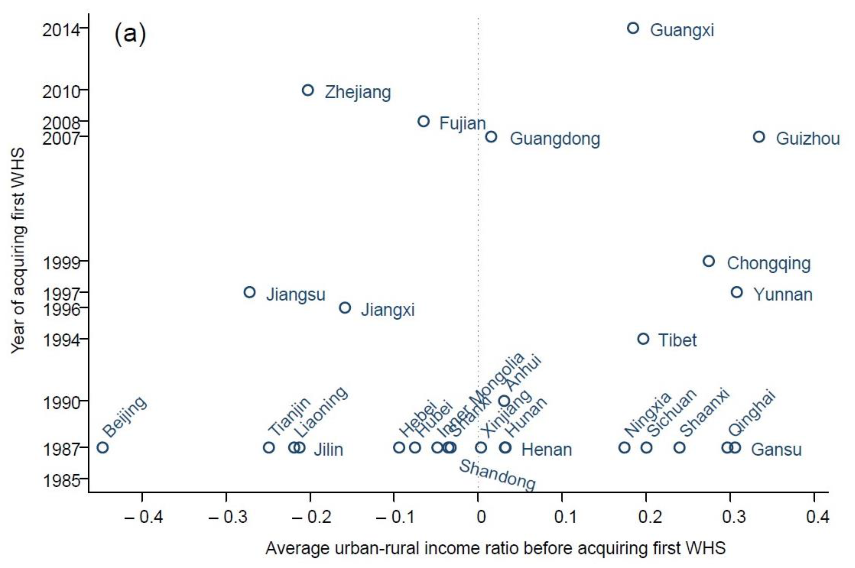
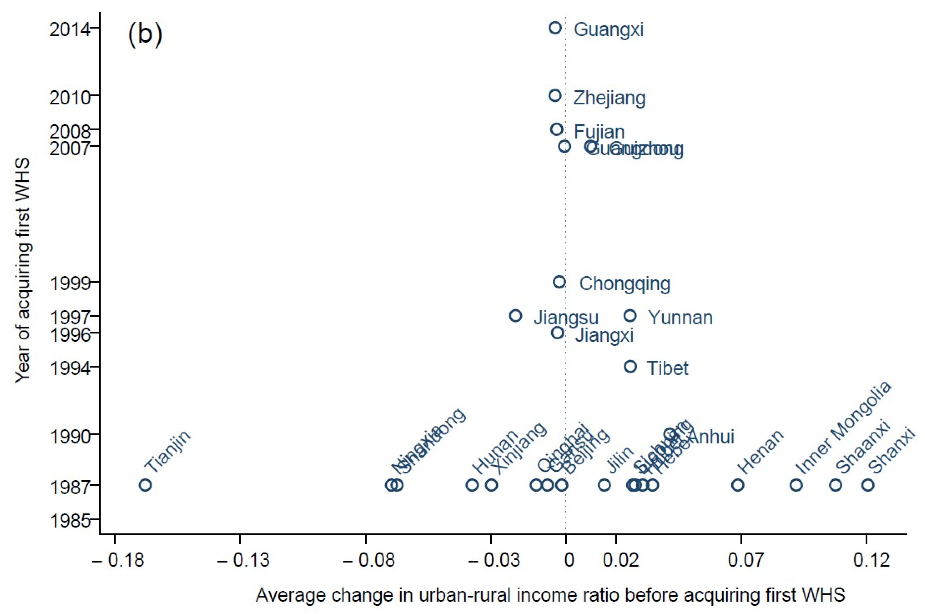
Secondly, the timing of successful application for WHS was unaffected by urban-rural income inequality.

Table A4. Years of acquiring World Heritage Sites (WHS).

Province	Name of World Heritage Sites (Year)
Anhui (3)	Mount Huangshan (1990); Ancient Villages in Southern Anhui–Xidi and Hongcun (2000); The Grand Canal (2014)
Beijing (6)	Peking Man Site at Zhoukoudian (1987); The Great Wall (1987); Imperial Palaces of the Ming and Qing Dynasties in Beijing and Shenyang (1987); Summer Palace, an Imperial Garden in Beijing (1998); Temple of Heaven: an Imperial Sacrificial Altar in Beijing (1998); Imperial Tombs of the Ming and Qing Dynasties (2003); The Grand Canal (2014)
Chongqing (4)	Dazu Rock Carvings (1999); South China Karst (2007; 2014)
Fujian (4)	Fujian Tulou (2008); China Danxia (2010); Mount Wuyi (2017); Kulangsu, a Historic International Settlement (2017)
Gansu (3)	The Great Wall (1987); Mogao Caves (1987); Silk Roads: the Routes Network of Chang’an-Tianshan Corridor (2014)
Guangdong (2)	Kaiping Diaolou and Villages (2007); China Danxia (2010)
Guangxi (2)	South China Karst (2014); Zuojiang Huashan Rock Art Cultural Landscape (2016)
Guizhou (4)	South China Karst (2007; 2014); China Danxia (2010); Tusi Sites (2015); Fanjingshan (2018)
Hebei (4)	The Great Wall (1987); Mountain Resort and its Outlying Temples, Chengde (1994); Imperial Tombs of the Ming and Qing Dynasties (2000); The Grand Canal (2014)
Henan (6)	The Great Wall (1987); Longmen Grottoes (2000); Yin Xu (2006); Historic Monuments of Dengfeng in “The Centre of Heaven and Earth” (2010); Silk Roads: the Routes Network of Chang’an-Tianshan Corridor (2014); The Grand Canal (2014)
Hubei (5)	The Great Wall (1987); Ancient Building Complex in the Wudang Mountains (1994); Imperial Tombs of the Ming and Qing Dynasties (2000); Tusi Sites (2015); Hubei Shennongjia (2016)
Hunan (4)	The Great Wall (1987); Wulingyuan Scenic and Historic Interest Area (1992); China Danxia (2010); Tusi Sites (2015)
Inner Mongolia (2)	The Great Wall (1987); Site of Xanadu (2012)
Jiangsu (4)	Classical Gardens of Suzhou (1997); Imperial Tombs of the Ming and Qing Dynasties (2003); The Grand Canal (2014); Migratory Bird Sanctuaries along the Coast of Yellow Sea-Bohai Gulf of China (Phase I) (2019)
Jiangxi (3)	Lushan National Park (1996); Mount Sanqingshan National Park (2008); China Danxia (2010)
Jilin (1)	The Great Wall (1987)
Liaoning (4)	The Great Wall (1987); Imperial Palaces of the Ming and Qing Dynasties in Beijing and Shenyang (2004); Imperial Tombs of the Ming and Qing Dynasties (2004); Capital Cities and Tombs of the Ancient Koguryo Kingdom (2004)
Ningxia (1)	The Great Wall (1987)
Qinghai (2)	The Great Wall (1987); Qinghai Hoh Xil (2017)
Shaanxi (3)	Mausoleum of the First Qin Emperor (1987); The Great Wall (1987); Silk Roads: the Routes Network of Chang’an-Tianshan Corridor (2014)
Shandong (4)	Mount Taishan (1987); The Great Wall (1987); Temple and Cemetery of Confucius and the Kong Family Mansion in Qufu (1994); The Grand Canal (2014)
Shanxi (4)	The Great Wall (1987); Ancient City of Ping Yao (1997); Yungang Grottoes (2001); Mount Wutai (2009)
Sichuan (6)	The Great Wall (1987); Huanglong Scenic and Historic Interest Area (1992); Jiuzhaigou Valley Scenic and Historic Interest Area (1992); Mount Emei Scenic Area, including Leshan Giant Buddha Scenic Area (1996); Mount Qingcheng and the Dujiangyan Irrigation System (2000); Sichuan Giant Panda Sanctuaries - Wolong, Mt Siguniang and Jiajin Mountains (2006)
Tianjin (2)	The Great Wall (1987); The Grand Canal (2014)
Tibet (1)	Historic Ensemble of the Potala Palace, Lhasa (1994)
Xinjiang (3)	The Great Wall (1987); Xinjiang Tianshan (2013); Silk Roads: the Routes Network of Chang’an-Tianshan Corridor (2014)
Yunnan (5)	Old Town of Lijiang (1997); Three Parallel Rivers of Yunnan Protected Areas (2003); South China Karst (2007); Chengjiang Fossil Site (2012); Cultural Landscape of Honghe Hani Rice Terraces (2013)
Zhejiang (4)	China Danxia (2010); West Lake Cultural Landscape of Hangzhou (2011); The Grand Canal (2014); Archaeological Ruins of Liangzhu City (2019)

Notes: Total number of WHS by 2019 are in parentheses of the first column. Sources are from Operational Guidelines for the Implementation of the World Heritage Convention, 2019. Available online: https://whc.unesco.org/en/guidelines (accessed on 31 December 2019).

provides the year of first WHS acquisition for each province. Figure A1 shows that neither the level of urban-rural income ratio before acquiring the first WHS nor its rate of change prior to acquiring the first WHS explains the timing of acquiring the first WHS. Panel (a) of Figure A1 shows a scatter plot of the average urban-rural income ratio before acquiring first WHS (year effect removed) and the year of acquiring first WHS. Panel (b) of Figure A1 shows a scatter plot of the average change in urban-rural income ratio before acquiring first WHS (year effect removed) and the year of acquiring first WHS. A larger value of urban-rural income ratio means greater income inequality. The t-statistics for the correlations in panel (a) and (b) of Figure A1 are 0.76 and −0.48, respectively).

Thirdly, the fact that urban-rural income ratio did not affect the year of acquiring the first WHS emerges from a hazard model analysis.

Table A6. Timing of first WHS acquisition and pre-existing urban-rural income ratio: A duration model.

	(1)	(2)	(3)	(4)
	Dep. Var.: (log) expected year to acquire first WHS
$Urban-rual income ratio$	0.002	0.002	0.001	−0.001
	(0.002)	(0.001)	(0.002)	(0.003)
$Population density$		−0.002 *	−0.002 *	−0.012
		(0.001)	(0.001)	(0.007)
$Proportion of employees$		0.0001	0.00002	0.0003
$in the tertiary industries$		(0.0001)	(0.0001)	(0.0002)
$GDP share of tertiary industries$			0.0001	−0.0001
			(0.0002)	(0.0003)
$Constant$	7.595 ***	7.594 ***	7.592 ***	7.607 ***
	(0.004)	(0.004)	(0.004)	(0.012)
Observations	246	246	246	195

Notes: A Weibul hazard model is estimated in each regression. Column 4 excludes provinces that acquired their (first) WHS in 1987. A province is dropped once it acquires its first WHS. Sample summary statistics are presented in Table A5 of Supplemental material. Robust standard errors are in parentheses. Superscripts *, **, and *** indicate statistical significance at the 10%, 5%, and 1% level respectively.

reports tests on whether urban-rural income ratio influences the likelihood that a province acquires its first WHS in a specific year given that it has not acquired any WHS yet. Our sample period begins in 1985, two years before China acquired its first WHS. Seventeen provinces acquired their first WHS in 1987—Beijing, Gansu, Hebei, Henan, Hubei, Hunan, Inner Mongolia, Jilin, Liaoning, Ningxia, Qinghai, Shaanxi, Shandong, Shanxi, Sichuan, Tianjin, and Xinjiang. By 2018, only three provinces had not yet had any WHS—Heilongjiang, Hainan, and Shanghai. Results reported in Table A6 indicate that the timing of first WHS acquisition does not vary with the urban-rural income ratio. Column 1 reports a regression with the urban-rural income ratio only, while columns 2 and 3 add numerous provincial-level control variables. Column 4 removes provinces that acquired their first WHS in 1987. The main concern here is that, after some provinces had acquired their first WHS in 1987, other provinces might increase their effort to apply for WHS, and the provinces with stronger willingness to improve urban-rural income inequality may also have stronger motivation to apply for WHS. However, coefficients of urban-rural income ratio are insignificant in all specifications.

Fourthly, the number of years after first WHS acquisition and urban-rural income ratio do not move together directly. We estimate a reduced form function relating the logarithm of urban-rural income ratio and the number of years after first WHS acquisition. In

Table A7. Direct effects of the number of years since first WHS acquisition on urban-rural income ratio.

	(1)	(2)	(3)	(4)
$Number of years after first WHS acquisition$	−0.003	−0.003	−0.004	−0.003
	(0.003)	(0.003)	(0.003)	(0.004)
$Growth rate of real GDP percapita$		−0.136	−0.118	−0.102
		(0.150)	(0.157)	(0.158)
$Unemployment rate$			0.038	0.039
			(0.027)	(0.027)
$\left(log\right) Inbound intl. tourism earnings$				−0.023
				(0.018)
$Constant$	1.003 ***	1.015 ***	0.906 ***	1.197 ***
	(0.077)	(0.076)	(0.094)	(0.267)
$R^2$	0.54	0.54	0.56	0.57

Notes: 651 observations in each regression. All regressions include province and year fixed effects. Robust standard errors are in parentheses. Superscripts *, **, and *** indicate statistical significance at the 10%, 5%, and 1% level respectively.

, column 1 reports the results of a regression with the number of years after first WHS acquisition only, while columns 2 and 4 control for numerous control variables, including growth rate of real GDP per capita, unemployment rate, logarithm of inbound international tourism earnings. The coefficients of the number of years after first WHS acquisition are not statistically significant in all regressions.

Lastly, the number of years after acquiring first WHS might be correlated with urban-rural income ratio through two channels. (1) As a historical and cultural attraction, provinces with WHS not only attract domestic tourism, but also appeal to international tourists [30]. The increase in inbound international tourism revenue will influence urban-rural income ratio directly or indirectly. On the one hand, international tourism may promote domestic tourism through better tourism infrastructure construction and enlarged tourism publicity. On the other hand, international tourism can also influence urban-rural income ratio through the aforementioned price, earnings and government transfer channels [20]. Controlling for international tourism revenues helps mitigate this problem. (2) More developed provinces might devote more economic and financial resources to improve their WHS applications, such as recruiting more experts to collect and prepare materials. While the two-way fixed-effect model employed in our study can control for initial economic conditions, it cannot control for unobserved province-specific and time-variant changes. Nevertheless, controlling for the growth rate of per capita gross provincial product helps alleviate this problem, because economically developed areas have more economic strength and financial resources to apply for World Cultural Heritage [12].

Regarding the second and the third IVs, road density (km/km²) and rail density (km/km²), there are three threats to the vadility. Firstly, there is a possible correlation between road/rail density and urban-rural income ratio through initial economic conditions. But the two-way fixed-effect model employed in our study is capable of mitigating this problem. Secondly, road/rail density may reflect the stage of economic development. However, including the growth rate of per capita gross provincial product helps condition out this impact. Finally, rail density also faces a unique threat to its validity. As the preferred transportation mode for most migrant workers, railway could influence the urban-rural income gap through the labor market. Due to this concern, we control for urban registered unemployment rate in most regressions.

4.3. Results of the First Stage

Table A1. First-stage results: WHS as instrument.

	(1)	(2)	(3)	(4)	(5)
$Number of years after first WHS acquisition$	0.058 ***	0.056 ***	0.058 **	0.036 ***	0.023 **
	(0.020)	(0.020)	(0.024)	(0.013)	(0.011)
$Growth rate of real GDP per capita$		0.108	0.530	0.680	−0.699
		(0.764)	(0.887)	(0.524)	(0.429)
$Unemployment rate$		−0.158 *	−0.161 *	−0.166 **	0.022
		(0.087)	(0.091)	(0.072)	(0.035)
$\left(log\right) Inbound intl. tourism earnings$		0.134	0.156	0.126	−0.037
		(0.110)	(0.131)	(0.105)	(0.064)
$Constant$	16.040 ***	14.750 ***	6.231 ***	8.391 ***	6.883 ***
	(0.477)	(1.536)	(1.816)	(1.342)	(0.883)
$R^2$	0.94	0.94	0.92	0.95	0.50
$F Statistic$	83.76	294.4	213.5	333.4	10.15

Notes: 651 observations in each regression. All regressions include province and year fixed effects. The dependent variable in columns 1 and 2 is logarithm of domestic tourism earnings. The dependent variable in column 3 is logarithm of domestic tourism earnings per capita. The dependent variable in column 4 is logarithm of number of domestic tourists. The dependent variable in column 5 is logarithm of average spending per domestic tourist. There is only one instrument, which is the number of years after first WHS acquisition. Robust standard errors are in parentheses. Superscripts *, **, and *** indicate statistical significance at the 10%, 5%, and 1% level respectively.

and

Table A2. First-stage results:Three instruments.

	(1)	(2)	(3)	(4)	(5)
$Number of years after first WHS acquisition$	0.059 ***	0.056 ***	0.058 **	0.036 ***	0.023 **
	(0.019)	(0.019)	(0.024)	(0.013)	(0.010)
$Road density$	−0.288	−0.302	−0.249	−0.032	−0.261 *
	(0.251)	(0.257)	(0.291)	(0.186)	(0.142)
$Rail density$	5.010	4.999	3.952	0.578	4.332 *
	(4.364)	(4.424)	(5.041)	(3.099)	(2.459)
$Growth rate of real GDP per capita$		0.072	0.501	0.676	−0.730
		(0.822)	(0.939)	(0.541)	(0.461)
$Unemployment rate$		−0.152 *	−0.158 *	−0.165 **	0.027
		(0.085)	(0.090)	(0.071)	(0.037)
$\left(log\right) Inbound intl. tourism earnings$		0.148	0.168	0.127	−0.026
		(0.111)	(0.133)	(0.105)	(0.067)
$Constant$	16.138 ***	14.691 ***	6.184 ***	8.384 ***	6.831 ***
	(0.410)	(1.532)	(1.821)	(1.342)	(0.904)
$R^2$	0.94	0.94	0.92	0.95	0.52
$F Statistic$	103.5	719	337.4	297.5	11.83

Notes: 651 observations in each regression. All regressions include province and year fixed effects. The dependent variable in columns 1 and 2 is logarithm of domestic tourism earnings. The dependent variable in column 3 is logarithm of Domestic tourism earnings per capita. The dependent variable in column 4 is logarithm of number of domestic tourists. The dependent variable in column 5 is logarithm of average spending per domestic tourist. There are three instruments, which are the number of years after first WHS acquisition, road density, and rail density. Robust standard errors are in parentheses. Superscripts *, **, and *** indicate statistical significance at the 10%, 5%, and 1% level respectively.

provide a number of first-stage specifications predicting domestic tourism development with the instrumental variables, and their impacts are quite strong and highly significant. Other supporting evidence are weak instrument test statistics developed by Stock and Yogo [37] and identification-robust confidence sets based on the Wald tests proposed by Andrews [38], which will be discussed in detail in Section 5. Overall, our instrumental variables are strong.

4.4. Alternative Specifications in Robustness Checks

We do robustness checks by using various specifications. Firstly, we use three alternative measures of tourism development: domestic tourism earnings per capita, the number of domestic tourists, average expenditure per domestic tourist. Specifically, $D_{pt}$ in Equation (1) represents these alternative domestic tourism measures in turn.

Secondly, after confirming the causal effect of domestic tourism on urban-rural income inequality, we provide in-depth analyses on whether the reduced urban-rural income inequality is due to the increase of rural residents’ income or the decrease of urban residents’ income. Specifically, $Z_{pt}$ in Equation (2) is the logarithm of urban or rural income for province p in year t.

$$Z_{pt}=\beta \times D_{pt}+\gamma \times X_{pt}+A_p+B_t+{\epsilon }_{pt}$$

(2)

4.5. Channels

According to Blake et al. [20], domestic tourism can influence urban-rural income ratio through three channels: price, earnings and government transfer. The price channel suggests that domestic tourism spending can lead to an increase in the relative prices of goods that poor households purchase. In China, rural households are generally poorer than urban households, and hence the price channel reduces the real income of rural residents. If the price channel works, the urban-rural income ratio would increase. Second, through the earnings channel, rural residents can benefit from higher wages and higher productions in tourism-related industries, which would consequently reduce the urban-rural income ratio. Finally, government transfers may depend on tourism-related revenues and therefore influence the urban-rural income ratio via redistribution. However, how government distribute revenue from domestic tourism to urban and rural households is uncertain. The urban-rural income ratio may increase or decrease depending on how the government transfer tourism revenue.

To assess the price channel, we estimate the impact of domestic tourism on food consumption. We make this choice for three reasons. First, food consumption in tourism can be “the peak touristic experience or the supporting consumer experience” [39], and hence food prices are more susceptible to domestic tourism than prices of other products and services. Usually, the prices of tradable goods are similar across locations, because they can be easily transported from high-price regions to low-price regions. On the other hand, non-tradable goods may exhibit large price differences across regions. In this sense, non-tradable goods should see the largest price effect, such as restaurant service. Second, changes in food prices would pose a greater effect on food consumption for low-income households within the region [40]. Third, Incera and Fernández [41] suggest that the price channel affects the poor by increasing prices of food and beverage, primary products, and real estate services, which are basic products for the poor.

Base on Equation (3), we conduct this exercise by examining the impact of domestic tourism on three variables regarding food prices. Specifically, $CHANNE{L}_{pt}$ in Equation (3) is (log) average food consumption expenditure of urban households, (log) average food consumption expenditure of rural households, or the (log) ratio of the two in province p in year t.

$$CHANNE{L}_{pt}=\beta \times D_{pt}+\gamma \times X_{pt}+A_p+B_t+{\epsilon }_{pt}$$

(3)

To investigate the earnings and the government channel, we focus on the impact of domestic tourism on four different types of disposable income of rural residents: wage, household operating income, net property income, and government transfer net income. Wage includes earnings from corporate and non-corporate organizations in local areas, and from work outside of the local areas. Local areas include local county or town. Household operating income comes from primary, secondary, and tertiary industries, respectively. Household operating income from primary industry include four parts: agriculture, forestry, livestock, and fishery. Household operating income from secondary industry is divided into manufacturing and construction. Household operating income from tertiary industry can be classified into four categories: (a) transportation, post, telecommunications, (b) wholesale, retail, trade, catering, (c) services, and (d) culture, education, health. These detailed data come from China Yearbook of Rural Household Survey (2001–2013), and the sample period is from 2000 to 2012. Specifically, $CHANNE{L}_{pt}$ in Equation (3) are the logarithm of the mean value of disposable income of rural residents or its various components in province p in year t.

5. The Effects of Domestic Tourism on Urban-Rural Income Ratio

Table 2. The effects of domestic tourism on urban-rural income ratio: Main results.

	(1)	(2)	(3)	(4)	(5)	(6)
	FE	FE	FEIV	FEIV	FEIV	FEIV
Variable			2SLS	2SLS	2SLS	2SLS
Dep. Var.: (log) urban-rural income ratio
$\left(log\right) Domestic tourism$	−0.062 *	−0.052 *	−0.054 ***	−0.053 ***	−0.060 ***	−0.059 ***
$earnings$	(0.038)	(0.036)	(0.021)	(0.022)	(0.023)	(0.024)
$Growth rate of real GDP$		−0.096		−0.096		−0.097
$per capita$		(0.159)		(0.099)		(0.098)
$Unemployment rate$		0.031		0.031 ***		0.030 ***
		(0.022)		(0.011)		(0.011)
$\left(log\right) Inbound intl.$		−0.016		−0.016 **		−0.015 *
$tourism earnings$		(0.017)		(0.009)		(0.009)
Instruments			$Years after first WHS$		$Years after first WHS$
					$Road/Rail densities$
First stage F statistics			80.00	72.21	29.80	26.75
Endogeneity test (p-value)			0.70	0.95	0.63	0.83
Cragg-Donald Wald F statistic			104.5	98.5	40.6	39.1
Hansan J (p-value)					0.59	0.84
Andrews (2018) Confidence Set			[−0.09, −0.01]	[−0.10, −0.01]	[−0.10, −0.02]	[−0.10, −0.01]
F statistic	44.17	46.31	41.92	40.84	42.56	41.26
$R^2 (within/centered)$	0.57	0.59	0.57	0.59	0.57	0.59

Notes: 651 observations in each regression. All regressions also include year fixed effects. Robust standard errors are in parentheses. Superscripts *, **, and *** indicate statistical significance at the 10%, 5%, and 1% level respectively.

reports the main results of the effects of domestic tourism on urban-rural income ratio. The dependent variable is the logarithm of urban-rural income ratio, and the key explanatory variable of interest is the logarithm of domestic tourism earnings. Column 1 reports a baseline FE model without any control variables. Column 3 reports the FEIV regression instrumented with the number of years after first WHS acquisition. Column 5 adds road and rail densities to the set of instruments and conducts over-identification tests. Columns 2, 4, and 6 are similar to columns 1, 3, and 5, respectively, but augmented with control variables including the growth rate of real GDP per capita, urban unemployment rate, and (log) international tourism earnings. The first stage F statistics are all larger than 10 in columns 3–6 (also see Table A1 and Table A2, columns 1 and 2). Cragg and Donald test statistics [37] also indicate that our instruments are not weak. Nevertheless, we construct weak-instrument-robust confidence set following Andrews (2018) to provide additional assurance. The instruments also pass conventional over-identification tests in columns 5 and 6. Note that the endogenous problem is not serious when using (log) domestic tourism earnings as domestic tourism indicator.

FE estimates reported in columns 1 and 2 show that higher domestic tourism earnings are associated with lower urban-rural income ratio, and the effects are statistically significant at 10% level. This, however, could be due to the endogeneity/reverse causality or omitted variable problems discussed above. Subsequent columns report results using various instrumental variables. We find that the FEIV estimates are statistically significant at 1% level, and the magnitudes are similar to FE estimates. Particularly in column 2, a 10% increase in domestic tourism earnings leads to a 0.52% decrease in urban-rural income ratio, only slightly smaller than the FEIV estimate reported in column 4 (−0.53) and column 6 (−0.59). Given that the average annual growth rate of domestic tourism earnings in our sample is about 20%, this predicts a 1.0–1.2% annual decrease in urban-rural income ratio.

Our results complement the study of Li et al. [42] where they find that domestic tourism reduces regional income inequality between more advanced region and the rest in China from 1997 to 2010. Li et al. [42] focus on inter-province income inequality, whereas we focus on intra-province income inequality. Therefore, our estimates are not directly comparable with theirs. They also find that domestic tourism makes a greater contribution than inbound international tourism. Shi et al. [29] find that a 10% increase in international tourism earnings leads to a 0.22% decrease in urban-rural income ratio in the local province. The logarithm of international tourism earnings is also included as a control variable in columns 2, 4, and 6. The coefficient estimate indicates that a 10% increase in international tourism earnings leads to a 0.16% decrease in urban-rural income ratio in the local province. This is quite similar to Shi et al. [29].

The role of domestic tourism in reducing urban-rural income inequality is reasonable. This can be explained by that there are more domestic tourists travelling in rural areas than in urban areas. For instance, the number of domestic tourists reached 5.54 billion in 2018, of whom 3 billion visited rural areas and 2.54 visited urban areas [43]. From the perspective of demand, due to rapid economic growth and urbanization, more and more urban residents started to seek slow-paced environments, enjoy the scene of diverse natural landscape in the countryside, and taste fresh farm produce [12]. From the perspective of supply, recreational agriculture and rural tourism are booming [44]. Originally, rural areas have tremendous tourism resources, such as diverse natural scenery, agricultural resources and traditional folk [45]. Recently, the central government has supported leisure agriculture and rural tourism boutique projects. The local government has constructed a large number of parks for leisure sightseeing and health regimen, and rural residents use their own space or build houses to provide private entertainment facilities (such as Nongjiale) [12,45].

However, more importantly, we find that domestic tourism plays a much more pronounced role in reducing urban-rural income inequality than international tourism. The limited share of international tourism in China so far [13] may explain the minor influence of international tourism than domestic tourism on alleviating income inequalities. In the short term, especially in the Post-COVID-19 era, the limited share of international tourism would remain [46], and the influence of international tourism would be still smaller than domestic tourism on alleviating income inequalities. In the long run, with the expansion of the international inbound tourism market, the role of international inbound tourism may converge with that of domestic tourism on reducing income inequalities.

6. Robustness of Main Results

6.1. Measurements of Domestic Tourism Development

In

Table 3. The effects of domestic tourism on urban-rural income ratio: Alternative measures of domestic tourism.

Variables	(1)	(2)	(3)	(4)	(5)	(6)
	FE	FEIV	FE	FEIV	FE	FEIV
		2SLS		2SLS		2SLS
Dep. Var.: (log) urban-rural income ratio
$\left(log\right) Domestic tourism earnings$	−0.048	−0.056 **
$per capita$	(0.030)	(0.022)
$\left(log\right) Number of domestic tourists$			−0.106 **	−0.086 **
			(0.041)	(0.035)
$\left(log\right) Average spending$					0.037	−0.120 **
$per domestic tourist$					(0.032)	(0.059)
$Growth rate of real GDP$	−0.076	−0.073	−0.033	−0.044	−0.060	−0.185 *
$per capita$	(0.169)	(0.100)	(0.175)	(0.100)	(0.168)	(0.107)
$Unemployment rate$	0.032	0.030 ***	0.022	0.025 **	0.037	0.042 ***
	(0.023)	(0.011)	(0.018)	(0.011)	(0.027)	(0.013)
$\left(log\right) Inbound intl.$	−0.016	−0.014	−0.009	−0.012	−0.026	−0.028 ***
$tourism earnings$	(0.017)	(0.010)	(0.019)	(0.010)	(0.016)	(0.008)
Endogeneity test (p-value)		0.854		0.405		0.003
Cragg-Donald Wald F statistic		33.02		22.73		21.73
Hansan J (p-value)		0.736		0.402		0.971
F statistic	46.55	41.62	46.75	43.86	48.71	32.96
$R^2 (within/centered)$	0.588	0.587	0.623	0.621	0.568	0.473

Notes: 651 observations in each regression. All regressions also include year fixed effects. In columns 2, 4, and 6, the instrumental variables are number of years since first WHS acquisition, road density, and rail density. Robust standard errors are in parentheses. Superscripts *, **, and *** indicate statistical significance at the 10%, 5%, and 1% level respectively.

, using alternative measures of domestic tourism development, we use Equation (1) to repeat the estimation presented in Table 2. Columns 1 and 2 use domestic tourism earnings per capita, and the results are very close to those reported in the baseline models. Columns 3 and 4 use number of domestic tourists, and the coefficients are around −0.1, about twice as strong as the impact of earnings. We find the largest impact (i.e., elasticities) in average expenditure per domestic tourist (column 6). A 10% increase in average expenditure per domestic tourist leads to a 1.2% decrease in urban-rural income ratio. Note that we only detect the endogeneity problem when average expenditure is used. In sum, alternative measures of domestic tourism development generally yield corroborating results. We also extended the baseline model in two directions. First, given that we have 21 years of data, the time-dimension is modestly long. We experimented with methods that are more robust to complex error structures and the results are presented in appendix

Table A8. Panel Data with Modest T and Alternative Error Structures.

Variable	(1)	(2)	(3)	(4)
$\left(log\right) Domestic tourism earnings$	−0.028 ***	−0.021 **	−0.062 ***	−0.052 ***
	(0.009)	(0.009)	(0.020)	(0.018)
$Growth rate of real GDP per capita$		−0.027		−0.096
		(0.047)		(0.142)
$Unemployment rate$		0.012 **		0.031 ***
		(0.006)		(0.012)
$\left(log\right) Inbound intl. tourism earnings$		−0.011 **		−0.016 *
		(0.006)		(0.011)
Number of observations	651	651	651	651
$R^2$	0.97	0.98	0.57	0.59

Notes: All regressions also include the province and year fixed effects. Columns 1–2 use the Prais-Winsten regression that allows for heteroskedastic and serially correlated error. Columns 3-4 report the Driscoll and Kraay [47] standard errors that are robust to general forms of spatial and temporal dependence. Standard errors are in parentheses. Superscripts *, **, and *** indicate statistical significance at the 10%, 5%, and 1% level respectively.

. Columns 1–2 use the Prais-Winsten regression that allows for heteroskedastic and serially correlated error, while columns 3–4 report the Driscoll and Kraay [47] standard errors that are robust to general forms of spatial and temporal dependence. The results are close to those reported in the baseline models. Moreover, following Machado and Santos Silva [48], we also explored heterogeneous impacts with a panel quantile regression approach, which is summarized in appendix

Table A9. Panel quantile regressions.

	Quantile
Variable	25th	50th	75th
Dep. Var.: (log) urban-rural income ratio
$\left(log\right) Domestic tourism earnings$	−0.036 *	−0.050 **	−0.070 *
	(0.025)	(0.026)	(0.050)
$Growth rate of real GDP per capita$	−0.172	−0.105	−0.015
	(0.196)	(0.208)	(0.401)
$Unemployment rate$	0.027 *	0.031 *	0.035
	(0.020)	(0.021)	(0.041)
$\left(log\right) Inbound intl. tourism earnings$	−0.014	−0.016	−0.019
	(0.015)	(0.016)	(0.031)

Notes: Estimation follows Machado and Santos Silva [48]. All regressions also include province and year fixed effects. Standard errors are in parentheses. Superscripts *, **, and *** indicate statistical significance at the 10%, 5%, and 1% level respectively.

. The impact at the median is similar to that at the mean, but the impact is twice as large at the 75th quantile than at the 25th quantile. That is, the positive impact of domestic tourism on reducing urban-rural income inequality is much stronger in provinces with more severe inequality.

6.2. Domestic Tourism and Income of Urban and Rural Residents

Although the results in Table 2 and Table 3 demonstrate that domestic tourism can reduce urban-rural income ratio, the analyses have not yet provided detailed information on whether the urban-rural income inequality shrinks because urban residents’ income falls, or because rural residents’ income rises faster. We now address this issue by evaluating the impact separately for urban and rural residents.

Table 4. The effects of domestic tourism on income of urban residents.

Variables	(1)	(2)	(3)	(4)	(5)
Dep. Var.: (log) disposable income of URBAN residents
$\left(log\right) Domestic tourism earnings$	0.035 *				0.043
	(0.019)				(0.035)
$\left(log\right) Domestic tourism earnings$		0.038 **
$perc apita$		(0.018)
$\left(log\right) Number of domestic tourists$			0.084 ***
			(0.031)
$\left(log\right) Average spending$				0.031
$per domestic tourist$				(0.038)
Endogeneity test (p-value)	0.419	0.353	<0.001	0.596	0.297
Cragg-Donald Wald ( F statistic)	39.11	33.02	22.73	21.73	13.91
Hansan J (p-value)	0.003	0.007	0.095	<0.001	0.006
$R^2 (within/centered)$	0.99	0.99	0.99	0.99	0.984

Notes: All regressions use the FEIV(2SLS) method and also include the growth rate of real GDP per capita, urban unemployment rate, (log) inbound international tourism earnings, and year fixed effects. The instrumental variables are number of years since first WHS acquisition, road density, and rail density. 651 observations in each regression of columns 1–4. In column 5, the sample period is from 2000 to 2012, and 403 observations in the regression. Robust standard errors are in parentheses. Superscripts *, **, and *** indicate statistical significance at the 10%, 5%, and 1% level respectively.

and

Table 5. The effects of domestic tourism on income of rural residents.

Variables	(1)	(2)	(3)	(4)	(5)
Dep. Var.: (log) disposable income of RURAL residents
$\left(log\right) Domestic tourism earnings$	0.094 ***				0.200 ***
	(0.019)				(0.040)
$\left(log\right) Domestic tourism earnings$		0.094 ***
$per capita$		(0.018)
$\left(log\right) Number of domestic tourists$			0.170 ***
			(0.033)
$\left(log\right) Average spending$				0.151 ***
$per domestic tourist$				(0.044)
Endogeneity test (p-value)	0.447	0.406	0.049	<0.001	<0.001
Cragg-Donald Wald (F statistic)	39.11	33.02	22.73	21.73	13.91
Hansan J (p-value)	0.027	0.042	0.578	0.001	0.344
$R^2 (within/centered)$	0.99	0.99	0.99	0.99	0.98

Notes: All regressions use the FEIV(2SLS) method and also include the growth rate of real GDP per capita, urban unemployment rate, (log) inbound international tourism earnings, and year fixed effects. The instrumental variables are number of years since first WHS acquisition, road density, and rail density. 651 observations in each regression of columns 1–4. In column 5, the sample period is from 2000 to 2012, and 403 observations in the regression. Robust standard errors are in parentheses. Superscripts *, **, and *** indicate statistical significance at the 10%, 5%, and 1% level respectively.

report estimated results of Equation (2) for urban and rural residents, respectively. Comparing the results across the two tables, we find that domestic tourism reduces urban-rural income ratio by raising rural residents’ income faster than that of urban residents.

That domestic tourism improves rural residents’ income more than urban residents’ income is vindicated across all four measures of domestic tourism development. A 10% increase in domestic tourism earnings increases the average disposable income of urban residents by 0.35% and that of rural residents by 0.94%. Columns 3 in both tables imply that a 10% increase in the number of domestic tourists leads to a 0.84% increase in average disposable income for urban residents, but it leads to a 1.70% increase for rural residents. These results will help us understand the channels analysis presented below.

7. Channels

7.1. Evidence on the Price Channel

Results in

Table 6. The effects of domestic tourism on food consumption (FC) of urban and rural residents.

	(1)	(2)	(3)	(4)	(5)	(6)
Dep. Var.	(log) FC		(log) FC Ratio
	Urban	Rural	Ratio of ${\mathit{FC}}_{\mathit{rural}}$ to ${\mathit{FC}}_{\mathit{urban}}$
Panel A: FE
$\left(log\right) Domestic tourism earnings$	0.201	0.006	−0.094 **
	(0.144)	(0.014)	(0.046)
$\left(log\right) Alternative domestic tourism measures$				−0.090 **	−0.096	−0.070 **
				(0.038)	(0.064)	(0.031)
Panel B: FEIV
$\left(log\right) Domestic tourism earnings$	0.247	0.067 **	−0.072
	(0.157)	(0.032)	(0.057)
$\left(log\right) Alternative domestic tourism measures$				−0.067	−0.105	−0.150
				(0.053)	(0.077)	(0.130)
$Durbin chi-squared test (p-value)$	0.54	<0.01	0.70	0.95	0.91	0.72
$Endogeneity test (p-value)$	0.354	0.018	0.361	0.292	0.774	0.492
$Cragg-Donald Wald F statistic$	39.11	39.11	39.11	33.02	22.73	21.73
$Hansan J test (p-value)$	0.541	0.216	0.345	0.320	0.360	0.282
$R^2 (within/centered)$	0.64	0.96	0.52	0.52	0.51	0.49

Notes: All regressions also include the growth rate of real GDP per capita, urban unemployment rate, (log) inbound international tourism earnings, and year fixed effects. Alternative measures of domestic tourism for columns 4–6 are domestic tourism earnings per capita, number of domestic tourists, and average spending per domestic tourist, respectively. The instrumental variables in Panel B include number of years since first WHS acquisition, road density, and rail density. 651 observations in each regression. Robust standard errors are in parentheses. Superscripts *, **, and *** indicate statistical significance at the 10%, 5%, and 1% level respectively.

show that domestic tourism does decrease real income of rural residents relative to urban residents through the food price channel. The p-values of endogeneity tests are all greater than 0.10, indicating we can focus on FE estimation results in panel A. Columns 3–6 show that domestic tourism earnings significantly decreases the ratio of average food consumption of rural residents to that of urban residents. This result is at odds with the study of Blake et al. [20]. They conjecture that via the price channel, tourism spending results in changes in prices for goods and services that poor households purchase in Brazil. A possible reason is that, in China, domestic tourists usually buy processed food, but residents generally buy unprocessed food. Also, rural residents with land can home-produce some food items such as rice, vegetables and meats, which allows them to stave off high market-prices at least partially.

7.2. Evidence on the Earnings Channel

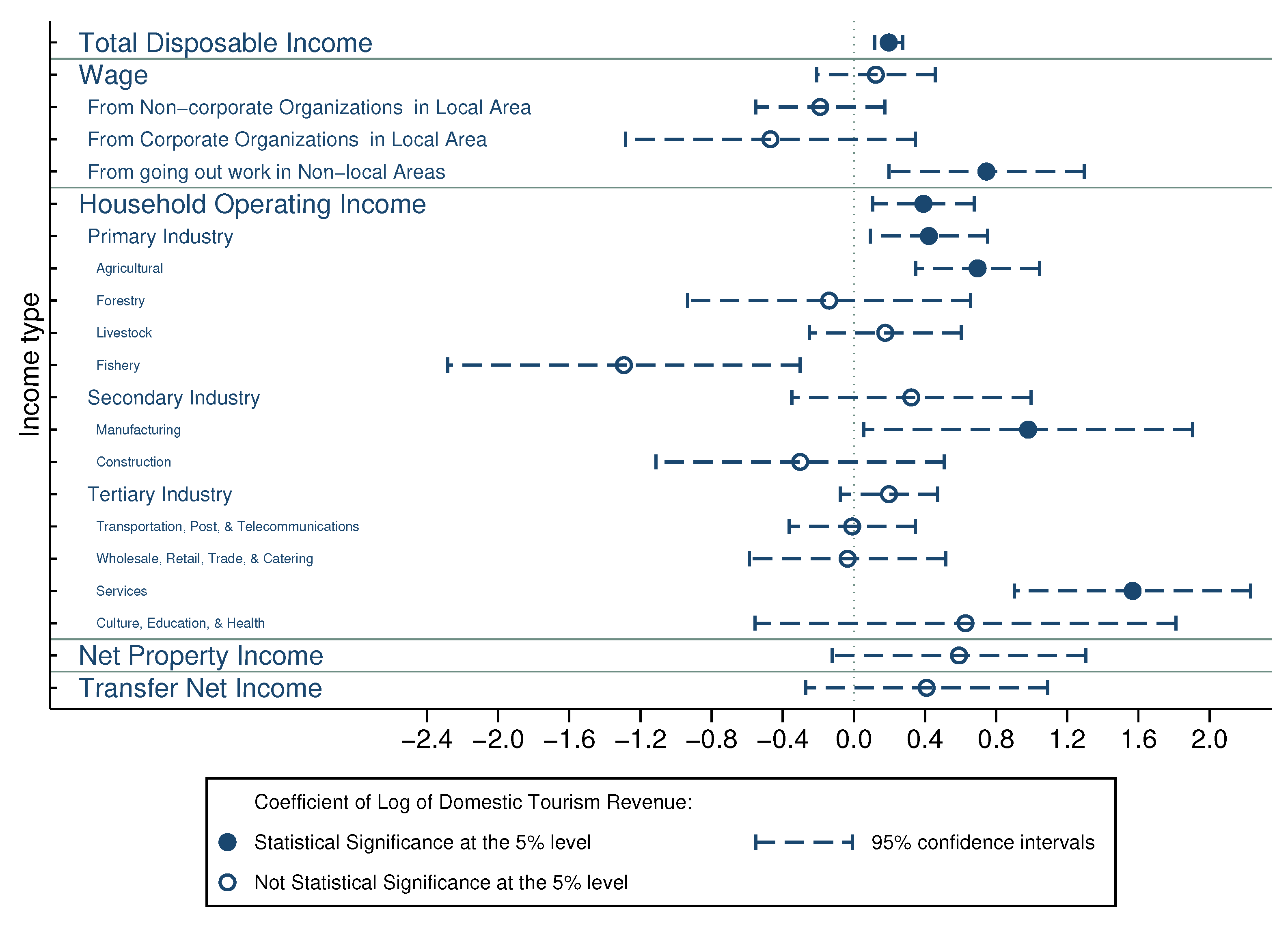
Figure 1 visualizes the coefficients of the logarithm of domestic tourism earnings from 2000 to 2012. Several observations can be made:

(1)

Domestic tourism earnings have indeed increased the disposable income of rural residents. A 10% increase in domestic tourism earnings leads to a 2% increase in the average disposable income of rural residents. Details of the result are also presented in column 5 of Table 5.

(2)

Zooming in on various components, a 10% increase in domestic tourism earnings is associated with a 7.5% increase in income from working outside of the local area.

(3)

A 10% increase in domestic tourism earnings leads to a 7% increase in rural residents’ average household operating income from agriculture. The results are in line with the analysis of Su et al. [49]. Using data from a town in Anhui Province of China from April 2015 to February 2016, they find that many rural households participate in tourism through selling tea and other agricultural tourism products. With the advent of e-commerce, tourists can continue to order agricultural products after their visit.

(4)

We do not find significant effect of domestic tourism earnings on household operating income from construction, although Su et al. [49] suggest that construction and renovation projects related to tourism could create job opportunities for rural residents.

(5)

We find a significant effect on household operating income from manufacturing. Manufacturing in this context usually refers to rural enterprises (These are rural enterprises with fixed places and production equipment, professional production labor force, and in production for more than three months in a year) that use hand and machinery to exploit natural resources, produce agricultural and sideline products, process and repair industrial products, and engage in handicraft industry (Handicraft industry refers to industrial production activities that rely on hand labor and use simple tools, including a variety of production, embroidery, weaving, carving, processing and other handicraft activities. The income of all products is calculated according to the processing fee. Self-made and self-used products are not included in the income). These products are likely to be purchased as specialty food, souvenir, or special tour goods.

(6)

Domestic tourism also significantly increases household operating income from services. A 10% increase in domestic tourism earnings leads to a 15.7% increase in rural residents’ average household operating income from services. These usually include income from finance and insurance, real estate management, hotels, car shops, hairdressing, photography, washing and dyeing, sewing, repair, tour guide, etc. This result is consistent with commonsense because these service activities are closely related to domestic tourism.

These evidences support the earnings channel. Figure 1 indicates that domestic tourism bolstered disposable income of rural residents, and mainly through increasing household operating income (from agriculture, manufacturing, and services). The strongest effects are found in services, followed by manufacturing and agriculture. We also use three alternative measures of domestic tourism to replace earnings, and the results are similar (Detailed results are not reported here to save space; they are available upon request).

7.3. Evidence on the Government Channel

Figure 1 also shows that domestic tourism earnings increase rural residents’ income from government transfers, but the effect is not statistically significant at conventional levels. According to Blake et al. [20], although domestic tourism can increase government revenue, the reallocation of this income stream is uncertain. They also suggest that government may spend the revenue on transfer payments to households, poverty relief programs, and the social service systems. This result is line with the result from Luo et al. [6]. They suggest that the rural poverty reduction in China is mostly due to income growth rather than redistribution.

The weak role of government transfers might be explained by the support system, regional variation and shifts in objectives on governance approaches. Firstly, without bottom-up accountability, transfer-based decentralisation would have limited impact on income redistribution. Although higher central transfers are useful to reduce interregional income inequalities, the equalising effects are only found for incomes of urban residents in China [50]. Secondly, as China is a developing country, the coordination of urban-rural balancing in different provinces may be difficult [51], which results in the insignificant role of government transfers. Thirdly, the objectives on governance approaches in different regions might not be same, such as national food security [52], rural-urban construction land equality [53], and farmers’ profits maximization [54].

8. Conclusions

This paper examines the causal effect of domestic tourism on urban-rural income inequality within 31 China’s provinces from 1998 to 2018. The results of the baseline model and robustness checks confirm that developing domestic tourism can reduce urban-rural income inequality. In-depth analyses illustrate that domestic tourism reduces the urban-rural income ratio by dis-proportionally raising the income of rural residents more than that of urban residents. The channels analyses find support for the earnings channel, but not for government transfer channels. The food price channel improves urban-rural income inequality in China.

The innovation of the current study is three-fold. First, this paper provides an unbiased estimate of the effect of domestic tourism on urban-rural income inequality by applying the instrumental variable method. Second, new evidence is provided on the role of domestic tourism in dis-proportionally raising the income of rural residents more than that of urban residents. Third, this study conducts in-depth channel analyses and empirically examines the channel theory of Blake et al. [20] regarding the role of tourism on poverty reduction in China.

Specifically, a 10% increase in domestic tourism earnings increases the average disposable income of urban residents by 0.35% and that of rural residents by 0.94%. Consequently, this leads to a reduction in the urban-rural income ratio by about 0.5–0.6%. Domestic tourism boosts the disposable income of rural residents mainly through increasing household operating income from agriculture, manufacturing and services.

In general, these results provide insights into the importance of domestic tourism policies and strategies for domestic tourism development in China. Firstly, the findings confirm the feasibility of reducing the income gap between urban and rural areas in the province through the development of domestic tourism. Secondly, any one of tourism indicators (domestic tourism earnings, domestic tourism earnings per capita, number of domestic tourists and average spending per domestic tourist) is applicable. Thirdly, strategies to increase domestic tourism supply are worth recommending, such as exploring diversified tourism products, expanding domestic tourist base, providing diversified and less seasonality tourism products as well as applying World Heritage Sites. Fourthly, there is still room for improvement in the redistribution of domestic tourism income by local governments. Lastly, technical guidance and financial services for rural residents to engage in domestic tourism are necessary.

There are several limitations to this study. Firstly, we only estimate the impact of domestic tourism on food consumption, which is only a preliminary exploration of the price channel. Further studies on consumption of other goods are needed. Secondly, the internal distribution across Chinese regions and movements within the country, including origin and distances of tourism streams might have a strong influence while investigating the role of domestic tourism. Future research on domestic tourism needs to consider the spatial effects of domestic tourism direction. Thirdly, the national and regional discourses on heritage appreciation might have a stronger influence than what is found from the quantitative analysis. In future work, we hope to move beyond the quantitative analysis and explore more underlining mechanisms by adopting qualitative analysis and case studies.

References

- Kuijs, L.; Wang, T. China’s Pattern of Growth: Moving to Sustainability and Reducing Inequality. China World Econ. 2006, 14, 1–14. [Google Scholar] [CrossRef]
- Xu, Y.; Zhang, T.; Wang, D. Changes in inequality in utilization of preventive care services: Evidence on China’s 2009 and 2015 health system reform. Int. J. Equity Health 2019, 18, 172. [Google Scholar] [CrossRef]
- Xue, Y.; Xuan, X.; Zhang, M.; Li, M.; Jiang, W.; Wang, Y. Links of family- and school-level socioeconomic status to academic achievement among Chinese middle school students: A multilevel analysis of a national study. Int. J. Educ. Res. 2020, 101, 101560. [Google Scholar] [CrossRef]
- Hou, C.; Tian, X.; Wang, S. A Bayesian analysis of parental education as instruments in estimating the return to schooling. Appl. Econ. Lett. 2020, 27, 113–117. [Google Scholar] [CrossRef]
- Sicular, T.; Ximing, Y.; Gustafsson, B.; Shi, L. The Urban-rural Income Gap and Inequality in China. Rev. Income Wealth 2007, 53, 93–126. [Google Scholar] [CrossRef] [Green Version]
- Luo, C.; Li, S.; Sicular, T. The long-term evolution of national income inequality and rural poverty in China. China Econ. Rev. 2020, 62, 101465. [Google Scholar] [CrossRef]
- Li, Y. Analysis on the disparity in economic growth and consumption between urban sector and rural sector of China: 1978–2008. Front. Econ. China 2010, 5, 559–581. [Google Scholar] [CrossRef]
- Benjamin, D.; Brandt, L.; Giles, J.; Wang, S. Inequality and Poverty in China during Reform (March 15, 2007). Poverty and Economic Policy Research Network Working Paper No. PMMA-2007-07. 2007, pp. 1–46. Available online: https://ideas.repec.org/p/lvl/pmmacr/2007-07.html (accessed on 3 August 2021).
- Molero-Simarro, R. Inequality in China Revisited. The Effect of Functional Distribution of Income on Urban Top Incomes, the Urban-Rural Gap and the Gini Index, 1978–2015. China Econ. Rev. 2017, 42, 101–117. [Google Scholar] [CrossRef]
- Yang, D.T. What has caused regional inequality in China? China Econ. Rev. 2002, 13, 331–334. [Google Scholar] [CrossRef]
- Yang, D.T.; Zhou, H. Rural-urban disparity and sectoral labour allocation in China. J. Dev. Stud. 1999, 35, 105–133. [Google Scholar] [CrossRef]
- World Tourism Organization. Domestic Tourism in Asia and the Pacific; UNWTO: Madrid, Spain, 2013. [Google Scholar]
- Ministry of Culture and Tourism of China. The Basic Situation of the Tourism Market in 2019; Ministry of Culture and Tourism of China: Beijing, China, 2020.
- Wu, B.; Zhu, H.; Xu, X. Trends in China’s domestic tourism development at the turn of the century. Int. J. Contemp. Hosp. Manag. 2000, 12, 296–299. [Google Scholar] [CrossRef]
- Williams, A.M.; Shaw, G. Tourism and Economic Development: Western European Experiences; Belhaven Press: London, UK, 1991. [Google Scholar]
- Liu, J.; Nijkamp, P.; Lin, D. Urban-rural imbalance and Tourism-Led Growth in China. Ann. Tour. Res. 2017, 64, 24–36. [Google Scholar] [CrossRef]
- Folarin, O.; Adeniyi, O. Does Tourism Reduce Poverty in Sub-Saharan African Countries? J. Travel Res. 2020, 59, 140–155. [Google Scholar] [CrossRef]
- Truong, V.D.; Hall, C.M.; Garry, T. Tourism and poverty alleviation: Perceptions and experiences of poor people in Sapa, Vietnam. J. Sustain. Tour. 2014, 22, 1071–1089. [Google Scholar] [CrossRef]
- McCulloch, N.; Winters, L.A.; Cirera, X. Trade Liberalization and Poverty: A Handbook; Centre for Economic Policy Research: London, UK, 2001. [Google Scholar]
- Blake, A.; Arbache, J.S.; Sinclair, M.T.; Teles, V. Tourism and poverty relief. Ann. Tour. Res. 2007, 35, 107–126. [Google Scholar] [CrossRef]
- Zhou, L.; Chan, E. Motivations of tourism-induced mobility: Tourism development and the pursuit of the Chinese dream. Int. J. Tour. Res. 2019, 21, 824–838. [Google Scholar] [CrossRef]
- Ma, T.; Hong, T.; Zhang, H. Tourism spatial spillover effects and urban economic growth. J. Bus. Res. 2015, 68, 74–80. [Google Scholar] [CrossRef]
- Zhang, J.; Zhang, Y. Tourism, economic growth, energy consumption, and CO2 emissions in China. Tour. Econ. 2020, 1–21. [Google Scholar] [CrossRef]
- Sofield, T.; Li, S. Tourism governance and sustainable national development in China: A macro-level synthesis. J. Sustain. Tour. 2011, 19, 501–534. [Google Scholar] [CrossRef]
- McBride, M. Relative-income effects on subjective well-being in the cross-section. J. Econ. Behav. Organ. 2001, 45, 251–278. [Google Scholar] [CrossRef]
- Jiang, S.; Lu, M.; Sato, H. Identity, Inequality, and Happiness: Evidence from Urban China. World Dev. 2012, 40, 1190–1200. [Google Scholar] [CrossRef] [Green Version]
- Asadullah, M.N.; Xiao, S.; Yeoh, E. Subjective well-being in China, 2005–2010: The role of relative income, gender, and location. China Econ. Rev. 2018, 48, 83–101. [Google Scholar] [CrossRef] [Green Version]
- Fang, J.; Gozgor, G.; Paramati, S.R.; Wu, W. The impact of tourism growth on income inequality: Evidence from developing and developed economies. Tour. Econ. 2020, 1–23. [Google Scholar] [CrossRef]
- Shi, W.; Luo, M.; Jin, M.; Cheng, S.K.; Li, K.X. Urban–rural income disparity and inbound tourism: Spatial evidence from China. Tour. Econ. 2020, 26, 1231–1247. [Google Scholar] [CrossRef]
- Patuelli, R.; Mussoni, M.; Candela, G. The effects of World Heritage Sites on domestic tourism: A spatial interaction model for Italy. J. Geogr. Syst. 2013, 15, 369–402. [Google Scholar] [CrossRef] [Green Version]
- Haddad, E.A.; Porsse, A.A.; Rabahy, W. Domestic tourism and regional inequality in Brazil. Tour. Econ. 2013, 19, 173–186. [Google Scholar] [CrossRef] [Green Version]
- Li, X.; Fu, H.; Wu, Y. Pollution mitigation, unemployment rate and wage inequality in the presence of agricultural pollution. China Econ. Rev. 2020, 61, 101425. [Google Scholar] [CrossRef]
- Carvalho, L.; Di Guilmi, C. Technological unemployment and income inequality: A stock-flow consistent agent-based approach. J. Evol. Econ. 2020, 30, 39–73. [Google Scholar] [CrossRef]
- Dwyer, L.; Forsyth, P.; Madden, J.; Spurr, R. Economic Impacts of Inbound Tourism under Different Assumptions Regarding the Macroeconomy. Curr. Issues Tour. 2000, 3, 325–363. [Google Scholar] [CrossRef]
- Khadaroo, J.; Seetanah, B. Transport infrastructure and tourism development. Ann. Tour. Res. 2007, 34, 1021–1032. [Google Scholar] [CrossRef]
- United Nations Educational, Scientific and Cultural Organization (UNESCO). Operational Guidelines for the Implementation of the World Heritage Convention; UNESCO World Heritage Centre: Paris, France, 2019. [Google Scholar]
- Stock, J.H.; Yogo, M. Testing for weak instruments in linear IV regression. In Identification and Inference for Econometric Models: Essays in Honor of Thomas Rothenberg; Cambridge University Press: Cambridge, UK, 2005; Volume 80. [Google Scholar]
- Andrews, I. Valid Two-Step Identification-Robust Confidence Sets for GMM. Rev. Econ. Stat. 2018, 100, 337–348. [Google Scholar] [CrossRef] [Green Version]
- Quan, S.; Wang, N. Towards a structural model of the tourist experience: An illustration from food experiences in tourism. Tour. Manag. 2004, 25, 297–305. [Google Scholar] [CrossRef]
- Green, R.; Cornelsen, L.; Dangour, A.; Turner, R.; Shankar, B.; Mazzocchi, M.; Smith, R. The effect of rising food prices on food consumption: Systematic review with meta-regression. BMJ Br. Med. J. 2013, 346, f3703. [Google Scholar] [CrossRef] [Green Version]
- Incera, A.C.; Fernández, M.F. Tourism and income distribution: Evidence from a developed regional economy. Tour. Manag. 2015, 48, 11–20. [Google Scholar] [CrossRef]
- Li, H.; Chen, J.L.; Li, G.; Goh, C. Tourism and regional income inequality: Evidence from China. Ann. Tour. Res. 2016, 58, 81–99. [Google Scholar] [CrossRef]
- Ministry of Agriculture and Rural Affairs of China. State Council’s Report on the Development of Rural Industries; Ministry of Agriculture and Rural Affairs of China: Beijing, China, 2019.
- Weng, G.; Pan, Y.; Li, J. Study on the Influencing Factors and Acting Path of the Sustainable Development of Rural Tourism Based on EEAM-ISM Model. Sustainability 2021, 13, 5682. [Google Scholar] [CrossRef]
- Chi, X.; Lee, S.K.; Ahn, Y.j.; Kiatkawsin, K. Tourist-Perceived Quality and Loyalty Intentions towards Rural Tourism in China. Sustainability 2020, 12, 3614. [Google Scholar] [CrossRef]
- Islam, M.M.; Fatema, F. Covid-19 and Sustainable Tourism: Macroeconomic Effect and Policy Comparison among Europe, the USA and China. Asian Bus. Rev. 2020, 10, 53–60. [Google Scholar] [CrossRef]
- Driscoll, J.C.; Kraay, A.C. Consistent Covariance Matrix Estimation With Spatially Dependent Panel Data. Rev. Econ. Stat. 1998, 80, 549–560. [Google Scholar] [CrossRef]
- Machado, J.A.; Santos Silva, J. Quantiles via moments. J. Econom. 2019, 213, 145–173. [Google Scholar] [CrossRef]
- Su, M.M.; Wall, G.; Wang, Y.; Jin, M. Livelihood sustainability in a rural tourism destination - Hetu Town, Anhui Province, China. Tour. Manag. 2019, 71, 272–281. [Google Scholar] [CrossRef]
- Fan, F.; Li, M.; Tao, R.; Yang, D. Transfer-based decentralisation, economic growth and spatial inequality: Evidence from China’s 2002–2003 tax sharing reform. Urban Stud. 2020, 57, 806–826. [Google Scholar] [CrossRef]
- Chen, C.; Legates, R.; Fang, C. From coordinated to integrated urban and rural development in China’s megacity regions. J. Urban Aff. 2019, 41, 150–169. [Google Scholar] [CrossRef]
- Anderson, K.; Strutt, A. Food security policy options for China: Lessons from other countries. Food Policy 2014, 49, 50–58. [Google Scholar] [CrossRef]
- Tan, R.; Wang, R.; Heerink, N. Liberalizing Rural-to-Urban Construction Land Transfers in China: Distribution Effects. J. Urban Aff. 2020, 60, 101147. [Google Scholar] [CrossRef]
- Zhang, Q.; Chen, Z.; Li, F. Appropriate Management Scale of Farmland and Regional Differences under Different Objectives in Shaanxi Province, China. Land 2021, 10, 314. [Google Scholar] [CrossRef]
Figure 1.
The coefficients of (log) domestic tourism earnings on income sources of rural residents: Graphical analysis (2000–2012).