Comparison of Snow Indices in Assessing Snow Cover Depth in Northern Kazakhstan

Abstract

This study compares the performances of four existing snow indices (Normalized-Difference Snow Index, Normalized-Difference Snow and Ice Index, Difference Snow Index, and Ratio Snow Index) in estimating snow cover depth at three agricultural enterprises in different soil zones, namely, the “North Kazakhstan Agricultural Experimental Station”, A.I. Barayev “Research and Production Center for Grain Farming”, and “Naidorovskoe”. From 30 January to 9 February 2022, the snow cover thickness and density were measured at 410 and 285 points, respectively, throughout the agricultural enterprise territories. It was found that: (1) snow-covered territories were effectively classified using all spectral indices except both combinations of RSI; (2) the snow cover fraction maps generated from DSI most accurately classified the non-snow areas as forest plantations, settlements, and strongly blown uplands; (3) the maps generated from DSI-2 presented a clear pattern of objects in all three study areas; (4) the liquid water in snowpacks is available in excess for possible reservation and rational use in agriculture during the dry season. At the “North Kazakhstan AES”, A.I. Barayev “Research and Production Center for Grain Farming”, and “Naidorovskoe”, the RMSE varied from 5.62 (DSI-2) to 6.85 (NDSII-2), from 3.46 (DSI-2) to 4.86 (RSI-1), and from 2.86 (DSI-2) to 3.53 (NDSII-1), respectively. The DSI-2-based snow depths best matched the ground truth, with correlations of 0.78, 0.69, and 0.80, respectively.

1. Introduction

Kazakhstan’s largest crop production areas are found in the northern and central regions, which permanently suffer from spring and summer droughts. The dry climate reduces crop yield and quality and lowers Kazakhstan’s socio-economic situation. Given the current realities of climate change and the agrarian practice of rainfed agriculture on the great steppe of Kazakhstan, spring melt water can be a primary source of water for irrigated agriculture. To do this, estimating the amount of snow and snow water equivalent and retaining melt water in small reservoirs is necessary. In addition, this decision would help prevent the annual spring floods of settlements. The region receives a stable amount of snow cover for up to six months a year, potentially allowing the use of melt water for agricultural purposes.

Methods for obtaining reliable, large-area snow cover information with high spatial and temporal resolution are essential because snow cover naturally has high spatio-temporal variability and shows rapid directional changes under the influence of climate change [1,2,3,4]. Owing to its extreme thermophysical characteristics, highly variable parameters, and duration of occurrence on vast land areas, snow cover affects almost all interactions between the atmosphere and the underlying surfaces at temperate and high latitudes in the cold season [5,6]. Climate warming causes earlier than normal snowmelt and shortens the period of stable snow cover, with adverse effects on natural and anthropogenic systems [7,8,9]. Mountainous regions and plains in temperate regions, where the snow cover is susceptible to temperature fluctuations, will most likely suffer from increased snow melting [10,11]. Regime changes in snow accumulation and snow melting alter the level of spring floods and increase the potential for evaporation, thus affecting water resources and the agriculture sectors that depend on them [12]. Snow cover is an essential water supply for plants, as it prevents freezing winter crops, perennial grasses, and the root systems of fruits and berries [13,14,15].

Researchers worldwide have estimated snow depth from ground observations, geographic information systems, and remote sensing. These investigations are primarily conducted from two perspectives: direct measurements of actual snow depth and indirect estimates using snow indices and modeling equations. From the first perspective, the Nordic Snow Radar Experiment (NoSREx) conducted by Lemmetyinen et al. [16] estimates the snow depth, snow density, and snow water equivalent (SWE) in real-time from gamma water instruments at intensive observation points. Gan et al. [17] compared two passive microwave-estimated snow depths with SWE retrievals from the Advanced Technology Microwave Sounder and the Advanced Microwave Scanning Radiometer 2. They proposed two equations for calculating the snow depth in forested and non-forested territories. Both products captured the temporal variability of the SWE at elevations lower than 900 m and snow depths lower than 20 cm well. Jenssen and Jacobsen [18] measured the snow depth, snow density, and SWE in Norway using an ultra-wide-band (0.7–4.5 GHz) radar mounted on an unmanned aerial vehicle (UAV). They found that pseudo-noise radar can measure snow depths up to 5.5 m with high precision (R > 0.92) [18]. However, the frequency–wavenumber migration algorithm proved insufficient for estimating the snow density, and system improvements were required. From the second perspective, various snow indices and snow cover fraction (SCF) equations have been proposed for snow depth estimation. Analogously to the ratio vegetation index and difference vegetation index, Lin et al. [19] employed the ratio snow index (RSI), the difference snow index (DSI), and the existing normalized-difference snow index (NDSI) to estimate the SCF in northwestern China. They discovered that an exponential fitting (R² > 0.79) outperforms the linear fitting (R² > 0.15). Romanov and Tarpley [20] found a strong correlation between snowpack depth and FSC. After fitting the relationship to an exponential equation and formulating a parametrization, they achieved a mean absolute error of 5 cm over the U.S. Great Plains and Canadian prairies [20]. Kim et al. [21] compared the abilities of three existing SCF equations, namely linear, quadratic and exponential functions of NDSI, to estimate snow depth over South Korea. Although the quadratic function obtained the lowest root mean squared error (RMSE = 2.37 cm), the authors recommended the linear equation (RMSE = 3.43 cm) because the error of the snow depth map calculated by the quadratic equation will increase when using satellite images with high snowfall [21]. Additionally, Dixit et al. [22] compared NDSI, NDSII, and S3 to delineate snow cover over the Beas River basin, India, and proposed a new Snow Water Index (SWI). According to their findings, S3 could delineate snow and non-snow pixels more accurately (89%) compared with NDSI (80%) and NDSII (85%). The S3 index has a huge advantage in assessing snow cover in the forest zone, combining Red, NIR, and SWIR bands. However, since the authors needed to minimize the snow-water mixing, they proposed SWI (overall accuracy 93%), which utilizes green, NIR, and SWIR bands.

Although there are methods for snow cover assessment, new approaches are needed in the steppe zone, where there is no snow–water, snow–vegetation, or snow–shadow mixing. Consistently, within the framework of this study, we set a goal to develop an approach that allows assessing the snow cover (1) over large areas (>10,000 ha), (2) with high temporal resolution (<7 days), and (3) without field snow surveys, which are time- and resource-consuming. This paper compares snow indices for estimating snow depth at three agricultural enterprises in different soil zones, namely, the limited liability partnerships (LLPs) North Kazakhstan Agricultural Experimental Station, A.I. Barayev Research and Production Center for Grain Farming, and Naidorovskoe. The selected snow indices were the NDSI, NDSII, DSI, and RSI from the Sentinel-2 multispectral instrument (MSI). The choice of these indices is justified because each has its advantages and disadvantages, which are suitable for use in the steppe zone and have not been compared before. NDSI is the most widely used snow index, which identifies snow cover by ignoring cloud cover and reducing the influence of atmospheric effects, while NDSII is used to determine not only snow cover, but also ice. In turn, knowing that snow density is greater than ice density, we intend to evaluate and compare the performance of NDSII in calculating the snow water equivalent. The use of such simple snow indices as DSI and RSI are bottomed because they are both susceptible to the amount of snow and can distinguish snow from soil differently. If DSI does not consider the difference between reflectance and radiance caused by the atmosphere or shadows, RSI takes advantage of the reduced influence of the atmosphere and topography. The modeled results were compared with actual snow survey results to assess the possibility of estimating the snowpack depth from the SCF–snow depth relationship. The objective of this study was to compare the snow depths estimated from the existing snow indices with parametrization in three different soil zones. The study outcomes form a scientific basis for early warning of spring floods, combating meteorological and agricultural droughts, and developing more accurate approaches for estimating snow depths over vast territories using geographic information systems (GISs) and remote sensing methods. Moreover, in addition to a new approach for snow cover assessment in the steppe zone, field snow survey data from three soil zones for independent testing and comparative studies by the international research community have been published under the CC BY license (see the Data Availability Statement).

2. Materials and Methods

2.1. Study Area

The study sites (see Figure 1) were three agricultural enterprises in different soil zones, the LLP North Kazakhstan Agricultural Experimental Station (Akkayin district, North Kazakhstan region), the LLP A.I. Barayev Research and Production Center for Grain Farming (Shortandy district, Akmola region) and the LLP Naidorovskoe (Osakarov district, Karagandy region). The climate is extremely continental and arid in all three regions, with hot summers and cold winters. The daily and annual temperatures fluctuate sharply. The average annual precipitation in the North Kazakhstan and Akmola regions is 350 mm, of which around 80% falls during the warm season (April–October). The Karaganda region receives only around 200 mm. Snow cover on the studied agricultural enterprises resides for approximately 150 days (November–March) and reaches average depths of 20–25 cm by the end of the winter season. Snow melt begins in mid-March and is completed at the end of April. The A.I. Barayev Research and Production Center for Grain Farming and the Naidorovskoe LLPs each have approximately 20,000 ha of cultivated land, while the North Kazakhstan Agricultural Experimental Station sows around 25,000 ha of arable land. Three main crop types are grown in the studied enterprises: cereals (wheat, oat, barley, and millet), legumes (peas, lentils, alfalfa, clover, and sweet clover), and oilseeds (safflower, sunflower, rapeseed, and flax). The sowing campaign typically begins in mid-May and ends in October.

2.2. Data Sources

2.2.1. In Situ Surveying

Field snow at the key sites was surveyed from 30 January to 9 February 2022 in the territories of the three agricultural enterprises (Figure 2). The snow cover thickness was measured at 410 points, and the snow density was measured at 285 points (

Table 1. Snow survey dates and numbers of measured points in the territories of the three limited liability partnerships.

Study Area/Snow Survey Dates and the Number of Points	30 January 2022		7 February 2022		9 February 2022
	Depth	Density	Depth	Density	Depth	Density
LLP North Kazakhstan Agricultural Experimental Station	118	118
LLP A.I. Barayev Research and Production Center for Grain Farming			144	19
LLP Naidorovskoe					148	148

).

The snow thickness was measured with a metal ruler with a 1 mm scale, and the snow density was calculated using a weight snow gauge (VS-43M). The actual snow density ρ (kg/m³) was calculated from the snow mass m (kg), the snow depth SD (m), and the area S (m²) of the VS-43M weight snow gage cylinder as

$$\rho =\frac{m}{SD\times S}$$

(1)

For convenient and quick movement in the study area, we operated our snowmobile (RM Vector 551i). To measure the actual snow height and density and determine the geolocation during snow surveys, we employed an M-103 II snow gage, a VS-43M weight snow gage, and a Garmin Montana 610 system (see Figure 3).

2.2.2. Digital Satellite Image Dataset

As the remote sensing data for estimating the snow cover thickness, we used wide-swath and high-resolution multispectral images of the Sentinel-2 MSI. Images with the nearest dates to the field-snow surveying dates were downloaded and processed. At the LLP North Kazakhstan Agricultural Experimental Station, the satellite images and field work dates coincided, but to cover the large territory of the study area, we constructed a mosaic of two satellite images with different cloud cover percentages. At the A.I. Barayev Research and Production Center for Grain Farming and Naidorovskoe, satellite images were taken four days earlier and two days later than the field-snow survey, respectively. The cloud coverage in the satellite image excluded the study area of the three agricultural enterprises.

Table 2. Specifications of the Sentinel-2 multispectral instrument.

Sensor	Acquisition Date	Spectral Band with Wavelet (µm)	Cloud Cover
Sentinel-2	30 January 2022, 42UWE	Coastal (0.443)	26%
		Blue (0.490)
	30 January 2022, 42UWF	Green (0.560)	60%
		Red (0.665)
	3 February 2022, 43UCR	Vegetation red edge (0.705)	1%
		Vegetation red edge (0.740)
	11 February 2022, 42UCX	Vegetation red edge (0.783)	84%
		Near-infrared (0.842)
		Vegetation red edge (0.865)
		SWIR-Cirrus (1.375)
		SWIR-1 (1.610)
		SWIR-2 (2.190)

provides the details of the Sentinel-2 MSI specifications. All satellite images were downloaded from the Google Earth Engine cloud-based geospatial platform.

2.3. Methodology

The methodology of the present study included selecting an appropriate study site, collecting satellite and ground data, applying snow cover indices, calculating SCF maps from the snow cover indices, and estimating snow depth and SWE (Figure 4). The accuracy of each snow depth map was assessed through field-data validation. All the computations and analysis were applied to the satellite images using the Google Earth Engine cloud-based geospatial platform, ERDAS IMAGINE was used for stack image generation, and the final maps were produced in Quantum GIS software.

2.3.1. Spectral Snow Indices

The spectral reflectivity of snow has a distinct spectral variability, being high in the green band of visible light (0.543–0.578 µm) and low in the shortwave infrared region (SWIR) (1.565–2.280 µm). Therefore, we can automatically detect and extract snow cover extent using various snow spectral indices [23,24,25,26,27]. As mentioned above, we adopted the NDSI, NDSII, DSI, and RSI (see

Table 3. Snow indices and their definitions.

Snow Index	For Sentinel 2 MSI	For Landsat 8 OLI
NDSI1	GreenB03 − SWIRB11/GreenB03 + SWIRB11	GreenB03 − SWIRB06/GreenB03 + SWIRB06
NDSI2	GreenB03 − SWIRB12/GreenB03 + SWIRB12	GreenB03 − SWIRB07/GreenB03 + SWIRB07
NDSII1	RedB04 − SWIRB11/RedB04 + SWIRB11	RedB04 − SWIRB06/RedB04 + SWIRB06
NDSII2	RedB04 − SWIRB12/RedB04 + SWIRB12	RedB04 − SWIRB07/RedB04 + SWIRB07
DSI1	GreenB03 − SWIRB11	GreenB03 − SWIRB06
DSI2	GreenB03 − SWIRB12	GreenB03 − SWIRB07
RSI1	GreenB03/SWIRB11	GreenB03/SWIRB06
RSI2	GreenB03/SWIRB12	GreenB03/SWIRB07

). Using the NDSI, we can not only distinguish snow from non-snow pixels, but can also reduce the effects of clouds, atmospheric noise, and geometric distortion [28,29]. In addition, the NDSI accounts for the topographic effect and can map snow in mountain shadows [27]. Hall et al. reported that the NDSII index produces the same results as NDSI [24]. The NDSII was developed in 2001 as a mapping index of snow and ice cover for the VGT sensor of the SPOT-4 satellite [30]. It has four spectral bands (blue, red, near-infrared, and shortwave infrared), and its spectral range is similar to that of the Sentinel-2 MSI. The NDSII recognizes that the expressions of snow reflectivity differ in the red and SWIR ranges. The DSI and RSI, developed by Lin et al. in 2012 [19], respectively, imitate the difference vegetation index and ratio vegetation index with particular modifications in the spectral bands. In addition, as the snow reflectance in the SWIR-1 (1.610 µm) and SWIR-2 (2.190 µm) spectral bands are very similar, another set of snow indices was generated by changing B11 of the Sentinel 2 MSI to B12.

2.3.2. Calculation of SCF

The SCF defines the share of snow-covered surfaces within each pixel and is the most crucial parameter for estimating snow depth. The SCF varies between 0 and 1 (0–100%). Thus, a pixel value of 0.91 means that 91% of the pixel area is covered with snow. The literature provides both direct and indirect SCF calculation methods. Indirect methods are based on the correlations between snow indices and SCF, whereas direct methods employ visual analysis of high- and medium-resolution images. As the NDSI is highly correlated with SCF, many authors develop their own analysis approaches. For instance, Salomonson and Appel proposed the following linear function [28]:

$$SCF=a+b\times NDSI$$

(2)

where a and b are constants equal to 0.06 and 1.21, respectively. Barton et al. proposed the quadratic function [31]:

$$SCF=a+b\times NDSI+c\times NDS{I}^2$$

(3)

where a, b, and c are constants optimized at 0.180, 0.371, and 0.255, respectively. Lin et al. proposed the exponential function [19]:

$$SCF=a+b\times {\mathrm{e}}^{c\times NDSI}$$

(4)

where a, b, and c are equal to −0.41, 0.571, and 1.068, respectively. As direct methods are more accurate than indirect methods for estimating snow cover, we here compared the performances of four existing snow indices using a mixed linear method with two variables representing the reflectivity of an entirely snow-covered surface and a bare surface. For this purpose, we adopted the formula developed by Romanov and Tarpley [20]:

$$SCF=\frac{R-Land}{Snow-Land}$$

(5)

where R is the observed visible reflectance of the scene, and Land and Snow are the reflectivity of land and snow, respectively. The error in the SCF estimation was 10–13% depending on the SCF value [32]. In this study, we used the SCF maps of the three different soil zones in North Kazakhstan, along with the four snow indices from Sentinel-2 MSI.

2.3.3. Estimation of Snow Depth and SWE

Romanov et al. found a high positive correlation between the SCF and SD. They proposed the following equation:

$$SD=e^{aSCF}-1$$

(6)

where a is a constant equal to 0.33. The projections of low-level plants through the snow cover dominantly affect the dependency of snow depth on SCF. Once the snowpack completely covers the greenery, the SCF no longer responds to additional increases in snow depth. Romanov and Appel reported that the snow cover given by Equation (6) reaches 100% at a snow depth of around 27 cm [20].

The SWE integrally characterizes the thickness and density of the snow cover. This indicator, which most fully characterizes the snow reserves in a particular area, can also clarify the water regime of rivers and lakes and the activation of erosion processes. In the current work, the SWE was simply determined as:

$$SWE=\rho \times SD$$

(7)

where SWE is in kg/m², ρ is in kg/m³, and SD is in m.

3. Results

As many maps were generated, we considered it prudent to limit our discussion to the “North Kazakhstan Agricultural Experimental Station”. The maps from A.I. Barayev “Research and Production Center for Grain Farming” and “Naidorovskoe” are displayed in Appendix A.

3.1. Calculation of the Snow Spectral Indices

As mentioned above, we analyzed Sentinel-2 MSI images using two variations of four spectral snow indices. Figure 5 displays the snow indices at the “North Kazakhstan Agricultural Experimental Station” (the spectral indices at A.I. Barayev “Research and Production Center for Grain Farming” and “Naidorovskoe” are presented in Figure A1 and Figure A2, respectively, of Appendix A).

All spectral indices except the RSI (misclassified area: 6241 ha or 4.8%) accurately classified the snow-covered territories. The RSI-1 and RSI-2 maps displayed many large and small spots, respectively, with larger values in the northeastern part of the study area. Such patterns cannot reflect the actual intensity of the snow cover in the three agricultural enterprises. To distinguish dry snow from snow crust formed by the thawing and subsequent freezing of snow or by wind compaction (wind crust), we employed the NDSI and NDSII indices. The significant density difference between dry snow and snow/wind crust will likely affect the SWE calculation. However, consistent with Hall et al. [23], the NDSI and NDSII gave the same results and did not distinguish between snow and crust (Figure 5), although they classified the snow-covered territories with satisfactory accuracy. Despite the blurry class outlines, both difference snow indices detected the precise contours of the areas completely covered with snow (untouched agricultural fields), snow-free areas (settlements), and areas partially covered with snow (agricultural fields after snow retention). Snow retention is the agricultural practice of retaining and accumulating snow on arable land, mainly in the fields of steppe and forest-steppe zones (Figure 6). This technique is designed to prevent freezing of the soil and wintering plants and increase soil moisture reserves.

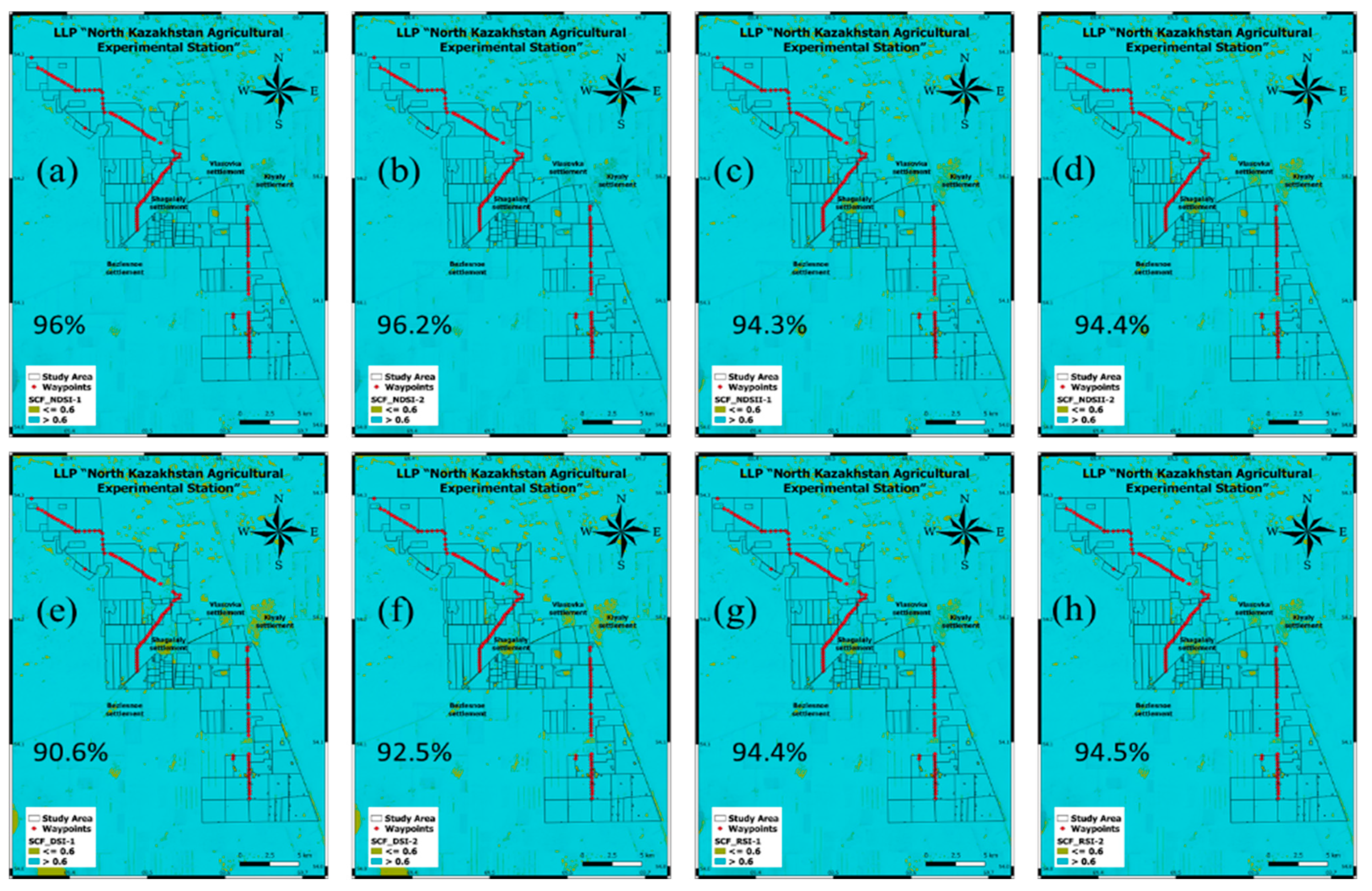
3.2. Estimation of SCF

Figure 7 shows the SCF maps at the “North Kazakhstan Agricultural Experimental Station” generated by inserting each snow index into the formula mentioned above (5). Equivalent maps at the A.I. Barayev “Research and Production Center for Grain Farming” and “Naidorovskoe” are displayed in Figure A3 and Figure A4 of Appendix A, respectively. As the SCF quantifies the share of a snow-covered area in each pixel, we calculated a single SCF value over the entire study area based on the pixel data. The SCF maps generated from the NDSII and RSI performed equally well and classified 94.3–94.5% of the land as totally snow-covered. At the “North Kazakhstan Agricultural Experimental Station”, the NDSI gave the highest snow coverage (96–96.2%), while DSI-1 and DSI-2 gave the smallest coverages (90.6% and 92.5%, respectively). It should also be noted that DSI most accurately classified non-snow areas as forest plantations, settlements, and strongly blown uplands. In the second study area located at A.I. Barayev “Research and Production Center for Grain Farming”, the NDSI and NDSII again obtained the highest proportion of snowed area (82–85.5%), followed by RSI (72.7–77.2%) and DSI (67–69.5%). In contrast, the “Naidorovskoe” territory was consistently classified as snow-covered (98.8–99.3%), although the DSI yielded the smallest share of snow-bound area (98.1–98.2%).

3.3. Snow Depth Modeling

Next, the snow depth maps were generated from each SCF map derived from the Sentinel-2 MSI data using Equation (6). Figure 8 displays the snow depth maps at the “North Kazakhstan Agricultural Experimental Station” (equivalent maps at A.I. Barayev “Research and Production Center for Grain Farming” and “Naidorovskoe” are presented in Figure A5 and Figure A6 of Appendix A, respectively). The height values in the snow depth map generated from NDSI and NDSII were similar between the variations, although NDSI-1 classified a larger snowy territory (depth > 30 cm) than NDSI-2 in the southeast part of “North Kazakhstan Agricultural Experimental Station”. The same behaviors were observed in A.I. Barayev “Research and Production Center for Grain Farming”, but in the “Naidorovskoe” territory, NDSI-2 classified the pixels more accurately than the other indices. In all three soil zones, the NDSI and NDSII obtained a blurry snow depth classification and failed to clarify the contours of the agricultural fields with and without snow retention. Meanwhile, both variations of RSI performed equally well in estimating SD in the three soil zones, and the pixel values were highly correlated with those in the snow depth maps derived from NDSII-1 and NDSII-2. The SD maps generated from DSI-1 showed the lowest depth values (0–10 cm) in the chernozem soil zone covering almost 80% of the study area, intermediate values in the chestnut soil zone (15–20 cm), and the highest value (51.4 cm) in the dark-chestnut soil zone. The most outstanding snow depth results, with clear object patterns in all three study areas, were obtained from DSI-2. No generalization of the pixel values was observed over the entire area, and fields with recently applied snow retention were easily distinguished as regions of partially visible snow–soil mixture (southern part of the study area; see Figure 8f). The DSI-2-derived map showed a larger area of 10–20-cm deep snow cover (>80%) than the other maps, while only specific fields (after recent snow retention), settlements, and hills were snow-free or thinly covered (0–10 cm).

The performances of the SCF maps generated from both variations of the four indices were compared in terms of the RMSEs and correlation coefficients (R) between the snow depths simulated using Equations (5) and (6) and the snow survey data collected in the field (

Table 4. Modeled snow depth error assessments.

Study Area	Error/Index	NDSII-2	NDSII-1	NDSI-2	NDSI-1	RSI-2	RSI-1	DSI-2	DSI-1
LLP “North Kazakhstan Agricultural Experimental Station”	R	0.45	0.2	0.53	0.24	0.55	0.25	0.78	0.51
	RMSE	6.85	7.45	6.44	7.02	6.16	6.66	5.62	7.29
LLP A.I. Barayev “Research and Production Center for Grain Farming”	R	−0.07	−0.01	−0.06	0	−0.06	0	0.69	0.5
	RMSE	4.75	4.69	4.84	4.67	4.85	4.86	3.46	4.1
LLP “Naidorovskoe”	R	0.26	0.18	0.44	0.41	0.44	0.4	0.80	0.51
	RMSE	3.47	3.53	3.4	3.5	3.27	3.35	2.86	3.17

). The RMSE decreased from the chernozem to the chestnut soil zones and varied from 5.62 (DSI-2) to 6.85 (NDSII-2) in the “North Kazakhstan Agricultural Experimental Station”, from 3.46 (DSI-2) to 4.86 (RSI-1) in the A.I. Barayev “Research and Production Center for Grain Farming”, and from 2.86 (DSI-2) to 3.53 (NDSII-1) in “Naidorovskoe”. The results of the DSI-2 model were most strongly correlated with the ground-truth snow depths in all three agricultural enterprises, with R values of 0.78, 0.69, and 0.80 in “North Kazakhstan Agricultural Experimental Station”, A.I. Barayev “Research and Production Center for Grain Farming”, and “Naidorovskoe”, respectively. At the latter two enterprises, the simulated snow depth from DSI-1 was the second-best match to the ground truth, but at the “North Kazakhstan Agricultural Experimental Station”, the snow depth was better modeled by RSI-2 (0.55) and NDSI-2 (0.53) than by DSI-1.

3.4. SWE Calculation

The SWE was calculated from each snow depth map using Equation (7). The SWE maps of the “North Kazakhstan Agricultural Experimental Station” generated from the snow depth maps of NDSI, NDSII, RSI, and DSI are displayed in Figure 9 (those of the A.I. Barayev “Research and Production Center for Grain Farming” and “Naidorovskoe” are displayed in Figure A7 and Figure A8 of Appendix A, respectively). Accurate SWE calculations require the snow densities in the steppe zone, which were averaged from our own data in each study area rather than extracted from the literature. The average snow density was 300 kg/m³ at “North Kazakhstan Agricultural Experimental Station” and 220 kg/m³ at A.I. Barayev “Research and Production Center for Grain Farming” and “Naidorovskoe”. This difference can be explained from a geographical viewpoint. The first study area is located in the forest-steppe zone, whereas the second is located in the steppe, and the third occupies the border between the steppe and the semi-desert zone. Comparing the SWE maps, all indices except DSI-2 underestimated the amount of snowpack water in all three soil zones. The SWE from DSI-2 exceeded 50 kg/m² over a large proportion of the “North Kazakhstan Agricultural Experimental Station”. In fields with recent snow retention, the SWE reduced to 20–40 kg/m², and in settlements and heavily blown hills, it varied between 0 and 20 kg/m².

In general, the liquid water contained in snowpacks at all three enterprises is available in surplus for potential agricultural reservation and rational use during the dry season. Moreover, the retained water could flood nearby communities and damage their infrastructures during a sudden spring thaw.

4. Discussion

The above results indicate that snow depths can be more accurately estimated using spectral snow indices from SCF maps than from previously proposed SCFs and snow depth estimation techniques. As mentioned, the SCF can be calculated either directly or indirectly. Salomonson and Appel [28], Barton et al. [31], and Lin et al. [19] proposed different regression functions based on NDSI. However, as direct methods are more accurate than indirect methods, we here compared the performances of four snow indices (NDSI, NDSII, DSI, and RSI) using two variables representing the reflectivities of an entirely snow-covered surface and a bare soil surface. In the NoSREx of Lemmetyinen et al. [16], the snow depth, snow density, and SWE NoSREx were automatically measured in real-time using a gamma water instrument at intensively observed points, but this work only characterized the snow cover at one or a few points. Although the study delivered the highest accuracy, its spatiality was very low. Furthermore, spatial interpolation will decrease the overall accuracy of the snow cover characteristics measured by NoSREx. Gan et al. [17] compared two passive microwave-obtained snow depths with SWE retrievals, but only achieved high accuracy for snow depths below 20 cm. Our present method increases this limit to 27 cm. Analogous work was performed by Jenssen and Jacobsen [18] in Norway. They measured the snow depth, snow density, and SWE using a UAV-mounted ultra-wide-band (0.7–4.5 GHz) radar. They found that pseudo-noise radar can measure the snow depth up to 5.5 m with high precision (R > 0.92). However, this method requires constantly repeated flights, which consumes time and resources; moreover, UAV flights are limited to smaller areas than those of our study (>10,000 ha). Regarding the work of Dixit et al., a comparative analysis of NDSI, NDSII, and S3 performance in assessing the snow cover in India was carried out, and the SWI index was proposed. Since SWI prevents the snow-water mixing and S3 averts the snow-vegetation mixing, they were excluded in the current study since this problem is not relevant in the steppe zone. Nevertheless, if the results of the snow cover assessment using NDSI and NDSII by Indian colleagues showed high accuracy, in our case, we observed an overestimation of these indices compared to DSI and RSI. Thus, according to the averaged Snow Cover Fraction data, NDSI classified 93% of the study area as snow-covered, and NDSII classified 92%. In comparison, DSI and RIS labeled only 86% and 89% of the area, respectively. Considering that DSI-2 showed the highest accuracy in snow depth estimation, we believe that NDSI and NDSII are less effective in assessing snow cover in Northern Kazakhstan. The approach we propose to use DSI-2 for snow cover depth estimation and further calculating the SWE can be used over a vast territory, with optimal temporal resolution (revisit time of Sentinel-2 is five days) and without field snow surveys.

Considering the advantages and limitations of estimating snow depths and SWE, we expect that our approach will be helpful for sustainable water management, the reservation and rational use of meltwater in agriculture during the dry season, and as an early warning system for spring floods.

5. Conclusions

All spectral indices except the RSI classified snow-covered territories with satisfactory performance. The NDSI and NDSII obtained the same results and did not distinguish between snow and crust. Both difference snow indices performed very well and clarified the completely snow-covered contours (untouched agricultural fields), snow-free areas (settlements, hills), and partially snow-covered areas (agricultural fields after snow retention) in the territory.

The SCF maps generated from NDSI and NDSII classified the highest proportion of the study area as snow-covered, whereas the maps generated from DSI-1 and DSI-2 identified the smallest share of snow-covered land. The SCF generated from DSI most accurately classified non-snow areas into forest plantations, settlements, and strongly blown uplands.

The RMSE between the simulated and surveyed snow depths decreased as the soil zone changed from chernozem to dark-chestnut. The snow depth maps generated from DSI-2 showed clear patterns of objects in all three study areas, and fields in which snow retention had been recently applied were easily identified as partially visible snow–soil mixtures. At the “North Kazakhstan Agricultural Experimental Station”, the A.I. Barayev “Research and Production Center for Grain Farming”, and “Naidorovskoe” areas, the RMSE varied from 5.62 (DSI-2) to 6.85 (NDSII-2), from 3.46 (DSI-2) to 4.86 (RSI-1), and from 2.86 (DSI-2) to 3.53 (NDSII-1), respectively, with DSI-2 yielding the highest correlation coefficients between the modeled and ground-truth data (0.78, 0.69, and 0.80, respectively).

The average snow density was 300 kg/m³ at “North Kazakhstan Agricultural Experimental Station” and A.I. Barayev “Research and Production Center for Grain Farming” and 220 kg/m³ at “Naidorovskoe”. The SWE maps generated from all indices except DSI-2 underestimated the amount of water in a snowpack. In general, the snowpacks in the study area contain surplus water that can be harnessed for reservation and rational use in agriculture during the dry season. Utilizing this water could also prevent flooding and damage to nearby communities during a sudden spring thaw.

The current study was limited to three agricultural enterprises in the North Kazakhstan, Aqmola, and Qaragandy regions and did not attempt a thorough investigation of all snow-covered regions in Kazakhstan. Further work will include a relief analysis and a methodology for choosing the best places for reserving melt and flood water in the northern regions of the Republic of Kazakhstan.

References

1. Armstrong, R.L.; Brun, E. Snow and Climate: Physical Processes, Surface Energy Exchange and Modeling; Cambridge University Press: Cambridge, UK, 2008; ISBN 978-0-521-85454-2. [Google Scholar]
2. Dong, C. Remote Sensing, Hydrological Modeling and in Situ Observations in Snow Cover Research: A Review. J. Hydrol. 2018, 561, 573–583. [Google Scholar] [CrossRef]
3. Lettenmaier, D.P.; Alsdorf, D.; Dozier, J.; Huffman, G.J.; Pan, M.; Wood, E.F. Inroads of Remote Sensing into Hydrologic Science during the WRR Era. Water Resour. Res. 2015, 51, 7309–7342. [Google Scholar] [CrossRef]
4. Sturm, M. White Water: Fifty Years of Snow Research in WRR and the Outlook for the Future. Water Resour. Res. 2015, 51, 4948–4965. [Google Scholar] [CrossRef]
5. Vavrus, S. The Role of Terrestrial Snow Cover in the Climate System. Clim. Dyn. 2007, 29, 73–88. [Google Scholar] [CrossRef]
6. Jones, H.G.; Pomeroy, J.W.; Walker, D.A.; Hoham, R.W. Snow Ecology: An Interdisciplinary Examination of Snow-Covered Ecosystems; Cambridge University Press: Cambridge, UK, 2001; ISBN 978-0-521-58483-8. [Google Scholar]
7. Duan, Y.; Luo, M.; Guo, X.; Cai, P.; Li, F. Study on the Relationship between Snowmelt Runoff for Different Latitudes and Vegetation Growth Based on an Improved SWAT Model in Xinjiang, China. Sustainability 2021, 13, 1189. [Google Scholar] [CrossRef]
8. Kumar, R.; Manzoor, S.; Vishwakarma, D.K.; Al-Ansari, N.; Kushwaha, N.L.; Elbeltagi, A.; Sushanth, K.; Prasad, V.; Kuriqi, A. Assessment of Climate Change Impact on Snowmelt Runoff in Himalayan Region. Sustainability 2022, 14, 1150. [Google Scholar] [CrossRef]
9. Mote, P.W.; Hamlet, A.F.; Clark, M.P.; Lettenmaier, D.P. Declining mountain snowpack in western North America. Bull. Am. Meteorol. Soc. 2005, 86, 39–50. [Google Scholar] [CrossRef]
10. Popova, V.V.; Morozova, P.A.; Titkova, T.B.; Semenov, V.A.; Cherenkova, E.A.; Shiryaeva, A.V.; Kitaev, L.M. Regional features of present winter snow accumulation variability in the North Eurasia from data of observations, reanalysis and satellites. Ice Snow 2015, 55, 73–86. [Google Scholar] [CrossRef] [Green Version]
11. Barnett, T.P.; Adam, J.C.; Lettenmaier, D.P. Potential Impacts of a Warming Climate on Water Availability in Snow-Dominated Regions. Nature 2005, 438, 303–309. [Google Scholar] [CrossRef]
12. Rood, S.B.; Pan, J.; Gill, K.M.; Franks, C.G.; Samuelson, G.M.; Shepherd, A. Declining Summer Flows of Rocky Mountain Rivers: Changing Seasonal Hydrology and Probable Impacts on Floodplain Forests. J. Hydrol. 2008, 349, 397–410. [Google Scholar] [CrossRef]
13. Groffman, P.M.; Driscoll, C.T.; Fahey, T.J.; Hardy, J.P.; Fitzhugh, R.D.; Tierney, G.L. Colder Soils in a Warmer World: A Snow Manipulation Study in a Northern Hardwood Forest Ecosystem. Biogeochemistry 2001, 56, 135–150. [Google Scholar] [CrossRef]
14. Pilon, C.E.; CÔté, B.; Fyles, J.W. Effect of Snow Removal on Leaf Water Potential, Soil Moisture, Leaf and Soil Nutrient Status and Leaf Peroxidase Activity of Sugar Maple. Plant Soil 1994, 162, 81–88. [Google Scholar] [CrossRef]
15. Zhang, T. Influence of the Seasonal Snow Cover on the Ground Thermal Regime: An Overview. Rev. Geophys. 2005, 43, 11. [Google Scholar] [CrossRef]
16. Lemmetyinen, J.; Kontu, A.; Pulliainen, J.; Vehviläinen, J.; Rautiainen, K.; Wiesmann, A.; Mätzler, C.; Werner, C.; Rott, H.; Nagler, T.; et al. Nordic Snow Radar Experiment. Geosci. Instrum. Methods Data Syst. 2016, 5, 403–415. [Google Scholar] [CrossRef] [Green Version]
17. Gan, Y.; Zhang, Y.; Kongoli, C.; Grassotti, C.; Liu, Y.; Lee, Y.-K.; Seo, D.-J. Evaluation and Blending of ATMS and AMSR2 Snow Water Equivalent Retrievals over the Conterminous United States. Remote Sens. Environ. 2021, 254, 112280. [Google Scholar] [CrossRef]
18. Jenssen, R.O.R.; Jacobsen, S.K. Measurement of Snow Water Equivalent Using Drone-Mounted Ultra-Wide-Band Radar. Remote Sens. 2021, 13, 2610. [Google Scholar] [CrossRef]
19. Lin, J.; Feng, X.; Xiao, P.; Li, H.; Wang, J.; Li, Y. Comparison of Snow Indexes in Estimating Snow Cover Fraction in a Mountainous Area in Northwestern China. IEEE Geosci. Remote Sens. Lett. 2012, 9, 725–729. [Google Scholar] [CrossRef]
20. Romanov, P.; Tarpley, D. Estimation of Snow Depth over Open Prairie Environments Using GOES Imager Observations. Hydrol. Process. 2004, 18, 1073–1087. [Google Scholar] [CrossRef]
21. Kim, D.; Jung, H.-S.; Kim, J.-C. Comparison of Snow Cover Fraction Functions to Estimate Snow Depth of South Korea from MODIS Imagery. Korean J. Remote Sens. 2017, 33, 401–410. [Google Scholar] [CrossRef]
22. Dixit, A.; Goswami, A.; Jain, S. Development and Evaluation of a New “Snow Water Index (SWI)” for Accurate Snow Cover Delineation. Remote Sens. 2019, 11, 2774. [Google Scholar] [CrossRef] [Green Version]
23. Hall, D.K.; Riggs, G.A.; Salomonson, V.V. Development of Methods for Mapping Global Snow Cover Using Moderate Resolution Imaging Spectroradiometer Data. Remote Sens. Environ. 1995, 54, 127–140. [Google Scholar] [CrossRef]
24. Hall, D.K.; Foster, J.L.; Verbyla, D.L.; Klein, A.G.; Benson, C.S. Assessment of Snow-Cover Mapping Accuracy in a Variety of Vegetation-Cover Densities in Central Alaska. Remote Sens. Environ. 1998, 66, 129–137. [Google Scholar] [CrossRef]
25. Hall, D.K.; Riggs, G.A.; Salomonson, V.V.; DiGirolamo, N.E.; Bayr, K.J. MODIS Snow-Cover Products. Remote Sens. Environ. 2002, 83, 181–194. [Google Scholar] [CrossRef] [Green Version]
26. Dozier, J. Spectral Signature of Alpine Snow Cover from the Landsat Thematic Mapper. Remote Sens. Environ. 1989, 28, 9–22. [Google Scholar] [CrossRef]
27. Negi, H.S.; Singh, S.K.; Kulkarni, A.V.; Semwal, B.S. Field-Based Spectral Reflectance Measurements of Seasonal Snow Cover in the Indian Himalaya. Int. J. Remote Sens. 2010, 31, 2393–2417. [Google Scholar] [CrossRef]
28. Salomonson, V.V.; Appel, I. Estimating Fractional Snow Cover from MODIS Using the Normalized Difference Snow Index. Remote Sens. Environ. 2004, 89, 351–360. [Google Scholar] [CrossRef]
29. Negi, H.; Kulkarni, A.; Semwal, B. Study of Contaminated and Mixed Objects Snow Reflectance in Indian Himalaya Using Spectroradiometer. Int. J. Remote Sens. 2009, 30, 315–325. [Google Scholar] [CrossRef]
30. Xiao, X.; Shen, Z.; Qin, X. Assessing the Potential of VEGETATION Sensor Data for Mapping Snow and Ice Cover: A Normalized Difference Snow and Ice Index. Int. J. Remote Sens. 2001, 22, 2479–2487. [Google Scholar] [CrossRef]
31. Barton, J.S.; Hall, D.K.; Riggs, G.A. Remote Sensing of Fractional Snow Cover Using Moderate Resolution Imaging Spectroradiometer (MODIS) Data. In Proceedings of the 57th Eastern Snow Conference, Syracuse, NY, USA, 2–3 June 2000; pp. 171–181. [Google Scholar]
32. Romanov, P. Mapping and Monitoring of the Snow Cover Fraction over North America. J. Geophys. Res. 2003, 108, 8619. [Google Scholar] [CrossRef]
Figure 1. Study area and soil map of the Republic of Kazakhstan.
Sustainability 14 09643 g001
Figure 2. Waypoints of snow survey over the territories of the three agricultural enterprises: (a) limited liability partnership (LLP) North Kazakhstan Agricultural Experimental Station, (b) LLP Naidorovskoe, and (c) LLP A.I. Barayev Research and Production Center for Grain Farming.
Sustainability 14 09643 g002
Figure 3. Process of measuring the snow height and density.
Sustainability 14 09643 g003
Figure 4. Flowchart of the data processing methods in the present study.
Sustainability 14 09643 g004
Figure 5. Spectral snow indices at “North Kazakhstan Agricultural Experimental Station”: (a) normalized-difference snow index [NDSI]-1, (b) NDSI-2, (c) normalized-difference snow and ice index [NDSII]-1, (d) NDSII-2, (e) difference snow index [DSI]-1, (f) DSI-2, (g) ratio snow index [RSI]-1, and (h) RSI-2.
Sustainability 14 09643 g005
Figure 6. Agricultural field at the “North Kazakhstan Agricultural Experimental Station” after applying the snow retention technique. Source: Captured by the authors during the field-snow survey.
Sustainability 14 09643 g006
Figure 7. Snow cover fraction (SCF) maps at the “North Kazakhstan Agricultural Experimental Station” generated from different snow cover indices: (a) NDSI-1, (b) NDSI-2, (c) NDSII-1, (d) NDSII-2, (e) DSI-1, (f) DSI-2, (g) RSI-1, and (h) RSI-2.
Sustainability 14 09643 g007
Figure 8. Snow depth maps at “North Kazakhstan Agricultural Experimental Station” generated from the SCFs of (a) NDSI-1, (b) NDSI-2, (c) NDSII-1, (d) NDSII-2, (e) DSI-1, (f) DSI-2, (g) RSI-1, and (h) RSI-2.
Sustainability 14 09643 g008
Figure 9. Snow water equivalent (kg/m2) maps of the “North Kazakhstan Agricultural Experimental Station” generated from the SDs of (a) NDSI-1, (b) NDSI-2, (c) NDSII-1, (d) NDSII-2, (e) DSI-1, (f) DSI-2, (g) RSI-1, and (h) RSI-2.
Sustainability 14 09643 g009