Using the Revised Universal Soil Loss Equation and Global Climate Models (CMIP6) to Predict Potential Soil Erosion Associated with Climate Change in the Talas District, Kazakhstan

Abstract

Changes in precipitation patterns, a fundamental aspect of climate change, can significantly impact soil erosion processes. This article aims to evaluate the current state of soil erosion in the Talas area utilizing the Revised Universal Soil Loss Equation (RUSLE). Climate projections for the study were obtained through the CMIP6 Global Climate Model (GCM) and the climatic data were integrated into the RUSLE to simulate potential changes in soil erosion patterns. The mean annual soil erosion rate, observed over the research duration, ranges from 0 to 127 (t y⁻¹). Results indicate that 56.29% of the study area is characterized by a low susceptibility to soil erosion, with an additional 33.56% classified as at moderate risk and 7.36% deemed at high risk of erosion. Furthermore, the evaluation reveals an average increase in precipitation levels compared to the baseline. Models project a rise of 21.4%, 24.2%, and 26.4% by the years 2030, 2050, and 2070, respectively. Concurrently, the study observes a parallel increase in soil loss with precipitation, demonstrating a rise of 34%, 35.5%, and 38.9% for the corresponding time periods. Also, the spatially distributed results show that the southern part of the territory of the Talas region has been impacted by erosion over the past and will also be in the future period. These findings underscore the intricate interplay between climate-induced changes in precipitation and their significant impact on soil erosion. The results provide essential insights for developing targeted soil conservation strategies in the Talas area under evolving climatic conditions.

1. Introduction

Soil erosion is an important environmental issue that has adverse effects on agricultural output, water quality, and the holistic well-being of ecosystems. Soil erosion occurs when particles of soil become dislodged and are subsequently transported from their original position to another location by the effect of natural factors such as wind, water, or other similar conditions. The issue of soil erosion has been a matter of concern since ancient times. However, due to the growth of agricultural practices and urban development, overexploitation, land abandonment, and agricultural intensification, it has evolved into a substantial worldwide problem [1,2,3,4,5]. Globally, estimated annual soil erosion of around 75 billion tons occurs, surpassing the natural erosion rate by a factor of 13–40 [6,7]. The susceptibility of Kazakhstan to soil erosion is significantly influenced by its geographical positioning and the prevailing arid to semi-arid climatic conditions [8]. Kazakhstan has an arid to semi-arid climate across various regions, with a notable concentration in the southern and central areas of the country [9]. These regions often have minimal annual precipitation levels, resulting in not enough soil moisture availability [10]. The concurrent occurrence of high temperatures and less precipitation may result in soil desiccation, hence making the soil more vulnerable to erosion [11]. Arid and semi-arid regions often have sparse vegetation cover due to water scarcity [12]. The lack of vegetation exposes the soil to the erosive forces of wind and water. Strong winds can lift and transport dry, loose soil particles over long distances. Kazakhstan’s open landscapes, especially in the steppe regions, provide ample opportunity for wind erosion to occur, leading to the loss of topsoil and degradation of agricultural land [13]. However, this research exclusively focuses on the modeling and discussion of water erosion, namely rainfall erosion. Rainfall-runoff erosivity refers to the ability of rainfall to cause soil erosion and contribute to runoff [14]. It is a crucial factor in soil erosion studies and is often assessed based on the characteristics of rainfall events [15]. In semi-arid regions, when rainfall does occur, it can sometimes be intense and sporadic. This can result in significant water erosion as runoff carries away soil particles. Additionally, when soil is already desiccated due to arid conditions, it becomes less capable of absorbing and retaining water, making it more prone to erosion during heavy rainfall events [16].

The dynamics of rainfall patterns are being modified by climate change [17,18,19]. The elevation in mean air temperature and alterations in weather patterns contribute to heightened intensity and irregular nature of rainfall episodes, hence augmenting the erosive capacity of precipitation. The impact of climate change on rainfall characteristics, including both strength and frequency, necessitates the integration of these alterations into soil erosion models [20,21]. Models are crucial tools for studying soil erosion at various scales, particularly when it comes to large geographic areas such as watersheds, regions, or even entire countries or continents [22]. The direct measurement and monitoring of soil erosion at these scales can be logistically challenging and expensive. Erosion models function as predictive tools for assessing soil loss, developing conservation strategies, conducting erosion surveys, and crafting project plans. Additionally, these models can serve as instruments to comprehend erosion processes and their implications [23]. Gaining a grasp of the principles behind constructing erosion models and the various types available can be beneficial for assessing model performance in diverse settings with different parameters. Among the commonly employed empirical erosion models are the Universal Soil Loss Equation (USLE) and the Revised Universal Soil Loss Equation (RUSLE) [24,25]. The RUSLE model, in particular, holds a central position in the natural resources field due to its extensive use and widespread acceptance, largely attributed to its user-friendly features [26]. The choice of the RUSLE model in this study is grounded in its simplicity of application, utilization of readily available data, and consistently accurate outcomes [27,28].

Climate change is one of the most pressing challenges of our time, with far-reaching implications for the environment, ecosystems, economies, and human societies. General circulation models (GCMs), also known as global climate models, play a crucial role in comprehending, simulating, and forecasting alterations in the Earth’s climate system [28,29]. GCMs are invaluable in this context, serving as powerful instruments for studying and projecting the effects of climate change on erosion and helping us develop strategies to mitigate its adverse impacts. Understanding these interactions is vital for our efforts to ensure a sustainable and resilient future. In order to assist climate change studies that necessitate more precise analysis, NASA established the NASA Earth Exchange Global Daily Downscaled Projections 6 (NEX-GDDP-CMIP6) initiative, which aims to furnish downscaled historical and prospective projections spanning from 1950 to 2100. These projections are derived from CMIP6 models. A comprehensive understanding of these interconnections is vital in our efforts to ensure a resilient and sustainable future [30,31,32].

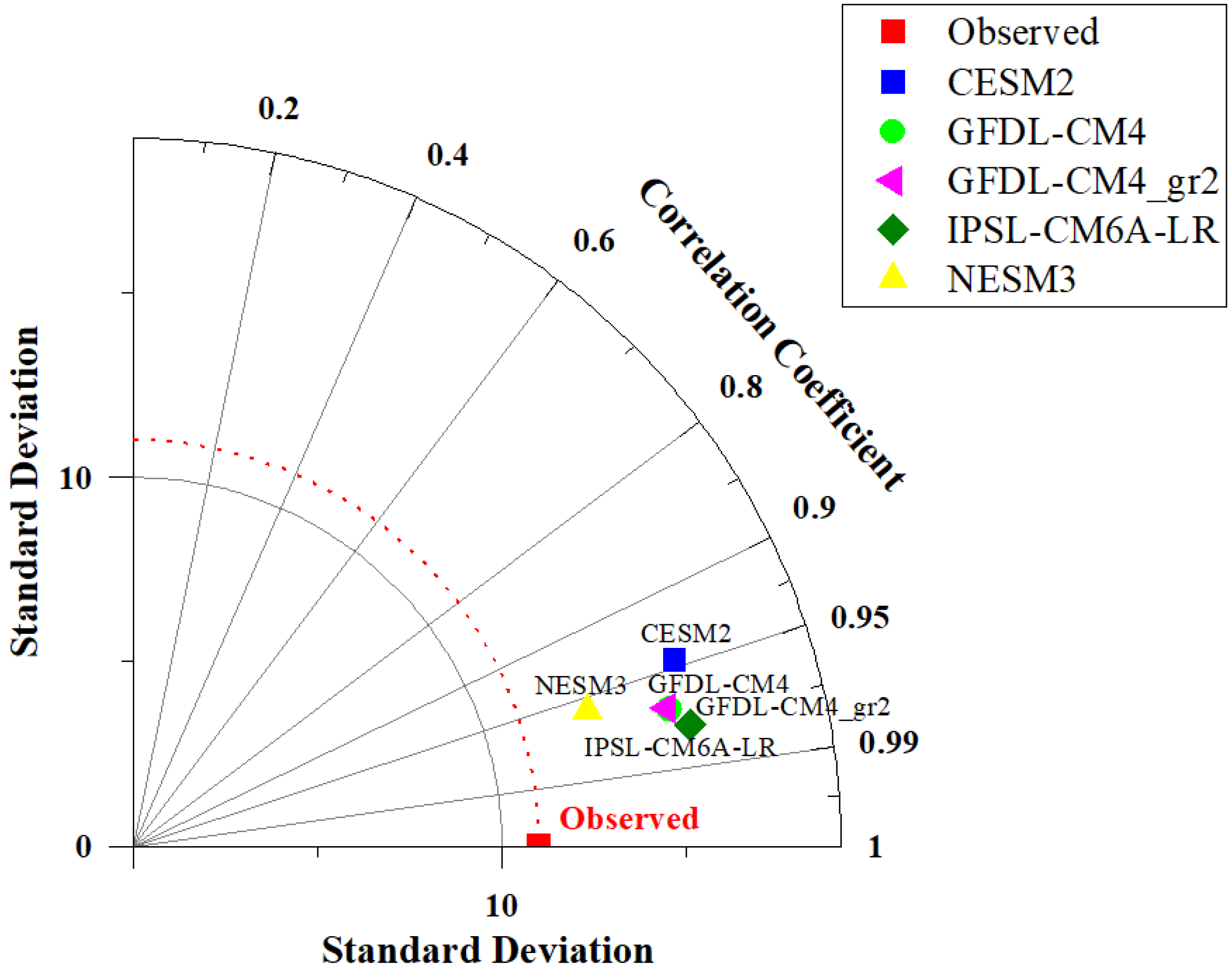
Multiple studies have investigated climate patterns in central Asia at different scales, employing various climate models. Gao et al. [33] assessed precipitation outputs from 30 global circulation models (GCMs) under the Coupled Model Inter-comparison Project Phase 6 (CMIP6) from 1951 to 2014, focusing on six climate zones in arid central Asia. Duulatov et al. [11] used GCMs from CMIP5 to assess rainfall changes for radiative concentration pathways (RCPs) 2.6 and 8.5. Ta et al. [34] employed CMIP5 to evaluate the ability of 37 GCMs to simulate historical precipitation in central Asia. Gulakhmadov [35] et al. used five GCMs from CMIP5 to project precipitation (Pr), maximum temperature (Tmx), and minimum temperature (Tmn) in the Vakhsh River Basin of CA for RCPs 4.5 and 8.5. Salehie et al. [36] selected CMIP6 GCMs to project climate changes over the Amu Darya River Basin. Gafforov et al. [37] utilized CMIP5 (RCPs 4.5 and 8.5) to evaluate the impact of climate change on rainfall-runoff erosivity in the Chirchik–Akhangaran Basin, Uzbekistan. Golian et al. [30] used CMIP6 models to assess future climate change effects on mine sites in Kazakhstan, considering Shared Socioeconomic Pathways (SSPs) 245 and 585. Lei et al. [38] evaluated CMIP6 models and a multi-model ensemble (MME) for extreme precipitation over arid central Asia. These studies collectively contribute to our understanding of climate variability and change in central Asia, utilizing a range of models, scenarios, and assessments focused on different aspects of the climate system. For the initial time in the Talas region, the study evaluates anticipated alterations in future precipitation using the recent CMIP6 models for the Revised Universal Soil Loss Equation (RUSLE). This approach aims to offer more comprehensive insights into potential future climate conditions in the Talas region. We utilize the latest CMIP6 models and including these updated models enhances the accuracy and relevance of our findings. By doing so, we seek to provide more targeted and region-specific information that can aid in informed decision making and adaptive strategies.

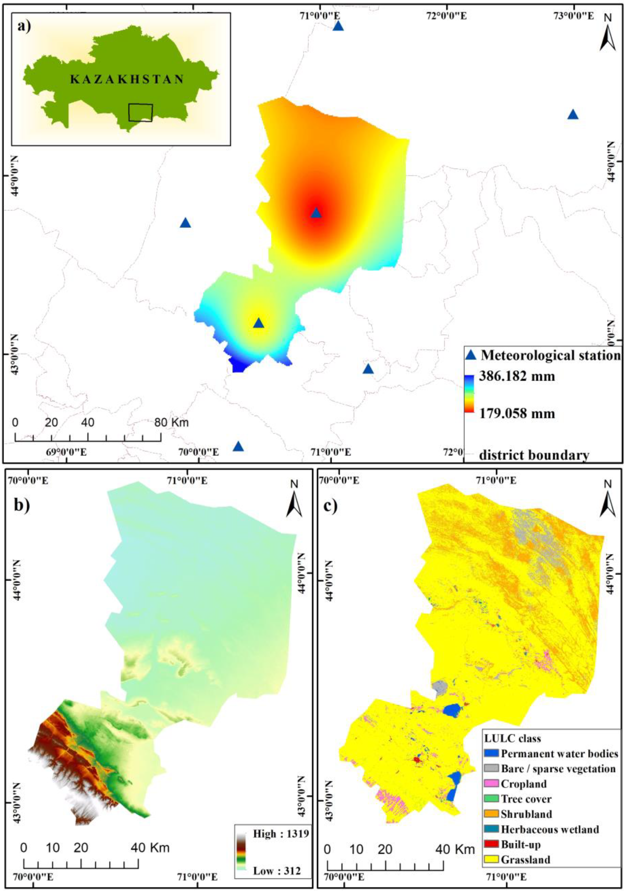
The purpose of this study is to assess the current state of soil erosion in the Talas region of Kazakhstan using the RUSLE model and a combination of global climate models under CMIP6. To the best of our knowledge, similar studies using a combination of the RUSLE model with CMIP6 have not yet been conducted in the Talas region of Kazakhstan in central Asia.

2. Materials and Methods

2.1. Study Area

The Talas district, with Karatau as its administrative center, is a constituent part of the Zhambyl region in the southern area of Kazakhstan. The district comprises a total of 24 settlements, which are organized into 13 rural districts. The study area possesses several distinctive geographical characteristics and is situated within the Talas district of the Zhambyl region. It encompasses the southwestern portion of the Moiynkum sandy desert, the Talas River valley, the piedmont hilly plains located between the Karatau Ridge and the Talas River valley, as well as the mountainous region consisting of the intermountain valley between the central Karatau Ridge and the Aktau. The research region is situated within the geographical coordinates of 42°48′ N to 44°27′ N and 69°55′ E to 71°37′ E. The whole land area is 12,200 square kilometers, with the Moiynkum sand massif accounting for 42.6% of the entire area, the piedmont hilly plains comprising 31.3%, the Talas River valley occupying 13.2%, and the mountainous region including 12.9% (Figure 1) [39]. The Talas region can be described in geomorphological terms as follows: the southern part is characterized by mountains, specifically the Karatau mountain range, while the northern part is predominantly flat, consisting of the accumulative and denudation plains of the Shu-Sarysu depression situated on the Turan plate [40]. The southwestern mountainous boundary of the region is characterized by the Karatau mountain system, which is a mid-mountain relief formed by tectonic denudation processes [41]. The soil and vegetation cover, as well as the current natural systems in the research region, are directly influenced by the prevailing meteorological conditions. The mountainous part of the region is characterized by arid mountain steppes situated atop undulating plains. The dominant soil types in the mountainous regions are mountain gray–chestnut and mountain gray soils. In the intermountain valleys, the predominant soil types are light northern gray soils and meadow gray soils. The soils in the flat region developed under arid desert circumstances and are characterized by meadow gray soils in the slopes. To the north, there are further occurrences of gray soils referred to as northern light gray soils. The valley of the Talas River contains meadow soils, which are occasionally accompanied by light brown tacro-like soils in certain areas. Moyynkum is a desert characterized by sandy terrain, where the absence of surface moisture hinders the development of soil, resulting in a predominance of sandy substrate. Depressions contain soils that are either takyr or takyr-like. The primary forms of vegetation consist of mountain wormwood, steppe grass, and phryganoids, which are upland xerophytes [41].

The climatic conditions of the Talas area are distinguished by significant annual and daily variations in surface air temperatures, as well as pronounced aridity. According to the Kazhydromet [42], the mean annual temperatures for 1980–2014 recorded at Uyuk and Moiynkum stations were +10.2 °C and +9.7 °C, respectively. The water resources within the region include the transboundary rivers Talas and Asa, as well as the mountain rivers Koktal and Tamdy. The majority of the region is situated in arid and semi-arid desert areas, resulting in a continental climate. The winter season is characterized by relatively low temperatures, while the summer season has high temperatures and arid conditions. The average air temperature in January is from −6 °C to 10 °C, and in July +24 °C to +27 °C. The average annual precipitation ranges from 140 to 230 mm [39].

2.2. Data

The current research provides a detailed summary of the key resources used in the inquiry, as shown in

Table 1. The types, sources, and quality of RUSLE input data used in this study.

Category	Source	Spatial Resolution	Temporal Period (Years)	Variables
DEM	ASTER (GDEM) V003	30 m	-	Elevation
Climate	Kazhydromet	-	1980–2014	35 y averaged annual precipitation
Soil	Harmonized World Soil Data (HWSD)	1 km	-	Sand, silt and clay fractions, organic matter (%)
Land cover	USGS Landsat 8	30 m	July 2021	Normalized Difference Vegetation Index NDVI
Land use	WorldCover 2021 v200	10 m	2021	Land use fraction

. Data were collected from a wide array of sources. The daily precipitation outputs were acquired from five GCMs in the CMIP6 archive. The present study utilizes a selection of GCMs including CESM2, GFDL-CM4, GFDL-CM4_gr2, IPSL-CM6A-LR, and NESM3 for the historical period 1980–2014, consistent with the observation period, as well as future climate data for the future period 2026–2100 according to two scenarios–SSPs 245 and 585. These GCMs were obtained from the NASA NEX-GDDP dataset, which has been specifically designed to align with the latest assessment report (AR6) published by the Intergovernmental Panel on Climate Change (IPCC). In comparison to the Coupled Model Intercomparison Project Phase 5 (CMIP5), CMIP6 showcases notable progress with the incorporation of a new set of emissions scenarios known as Shared Socioeconomic Pathways (SSPs) [33,43,44,45]. The data were subjected to a statistical downscaling procedure in order to achieve a higher level of resolution. The statistical downscaling strategy used in this study is the daily bias correction and spatial disaggregation (BCSD) method. The NEX-GDDP-CMIP6 dataset offers comprehensive worldwide coverage, with a spatial resolution of around 0.25° (equal to around 25 km). This dataset covers the time period from 1950 to 2100, encompassing both historical and forecasted periods. A comprehensive explanation can be found in

Table A1. List of general circulation models (GCMs) from the CMIP5 experiment utilized in this study.

Name of GCM	Institute	Horizontal Resolution (Lat. × Long.)
ACCESS-CM2	Commonwealth Scientific and Industrial Research Organization/Australia	0.25 × 0.25
ACCESS-ESM1-5	Commonwealth Scientific and Industrial Research Organization/Australia	0.25 × 0.25
BCC-CSM2-MR	Beijing Climate Center China Meteorological Administration/China	0.25 × 0.25
CanESM5	Canadian Centre for Climate Modelling and Analysis/Canada	0.25 × 0.25
CESM2	Community Earth System Model contributors, United States	0.25 × 0.25
CESM2-WACCM	Centre National de Recherches Météorologiques, France	0.25 × 0.25
CMCC-CM2-SR5	Fondazione Centro Euro-Mediterraneo sui Cambiamenti Climatici (CMCC), Lecce, Italy	0.25 × 0.25
CMCC-ESM2	Fondazione Centro Euro-Mediterraneo sui Cambiamenti Climatici (CMCC), Lecce, Italy	0.25 × 0.25 0.25 × 0.25 0.25 × 0.25
CNRM-CM6-1	Centre National de Recherches Météorologiques-Centre Européen de Recherche et de Formation Avancée en Calcul Scientifique/France	0.25 × 0.25
CNRM-ESM2-1	Centre National de Recherches Météorologiques-Centre Européen de Recherche et de Formation Avancée en CalculScientifique/France	0.25 × 0.25 0.25 × 0.25
EC-Earth3	EC-EARTH consortium/Europe	0.25 × 0.25
EC-Earth3-Veg-LR	EC-EARTH consortium/Europe	0.25 × 0.25 0.25 × 0.25
FGOALS-g3	Chinese Academy of Sciences/China	0.25 × 0.25 0.25 × 0.25
GFDL-CM4 (gr1)	NOAA Geophysical Fluid Dynamics Laboratory/USA	0.25 × 0.25
GFDL-CM4 (gr2)	NOAA Geophysical Fluid Dynamics Laboratory/USA	0.25 × 0.25
GFDL-ESM4	NOAA Geophysical Fluid Dynamics Laboratory/USA	0.25 × 0.25
GISS-E2-1-G	NASA’s Goddard Institute for Space Studies, United States	0.25 × 0.25
HadGEM3-GC31-LL	Met Office Hadley Centre/UK	0.25 × 0.25
HadGEM3-GC31-MM	Met Office Hadley Centre/UK	0.25 × 0.25
IITM-ESM2		0.25 × 0.25
INM-CM4-8	Institute for Numerical Mathematics, Russian Academy of Science/Russia	0.25 × 0.25
INM-CM5-0	Institute for Numerical Mathematics, Russian Academy of Science/Russia	0.25 × 0.25
IPSL-CM6A-LR	L’Institut Pierre-Simon Laplace/France	0.25 × 0.25
KACE-1-0-G	National Institute of Meteorological Sciences/Korea Meteorological Administration, Climate Research Division, Republic of Korea	0.25 × 0.25
KIOST-ESM	Korea Institute of Ocean Science and Technology (KIOST), Busan, Republic of Korea	0.25 × 0.25
MIROC-ES2L	Japan Agency for Marine-Earth cience and Technology, Atmosphere and Ocean Research Institute, The University of Tokyo, National Institute for Environmental Studies, and RIKEN Center for Computation al Science/Japan	0.25 × 0.25
MIROC6	Japan Agency for Marine-Earth Science and Technology, Atmosphere and Ocean Research Institute, The University of Tokyo, National Institute for Environmental Studies, and RIKEN Center for Computation al Science/Japan	0.25 × 0.25
MPI-ESM1-2-HR	Max Planck Institute for Meteorology/Germany	0.25 × 0.25
MPI-ESM1-2-LR	Max Planck Institute for Meteorology/Germany	0.25 × 0.25
MRI-ESM2-0	Meteorological Research Institute/Japan	0.25 × 0.25
NESM3	Nanjing University of Information Science and Technology/China	0.25 × 0.25
NorESM2-LM	Norwegian Climate Centre/Norway	0.25 × 0.25
NorESM2-MM	Norwegian Climate Centre/Norway	0.25 × 0.25
TaiESM1	Research Center for Environmental Changes, Academia Sinica, Nankang, Taipei, Taiwan	0.25 × 0.25
UKESM1-0-LL	Met Office Hadley Centre/UK	0.25 × 0.25

of Appendix A.

2.3. Metodology

The Revised Universal Soil Loss Equation (RUSLE) is a significant method utilized for the assessment and evaluation of soil erosion risks in the fields of land management, soil conservation, and environmental planning. The model incorporates various soil erosion parameters and integrates them into a unified equation to generate an estimate of potential soil loss. The RUSLE equation underwent development and refinement by several authors and researchers, such as Wischmeier and Smith [25,46], with a subsequent modification by Renard and Foster [47]. The essential components of the RUSLE model are as follows:

A = R × K × LS × C × P

(1)

where (A) represents the estimated average annual soil loss (t ha⁻¹ y⁻¹). The potential for soil erosion caused by rainfall and its intensity are measured by the rainfall erosivity factor (R) (MJ mm ha⁻¹ h⁻¹ y⁻¹). The soil’s sensitivity to erosion is indicated by the soil erodibility factor (K) (t ha h ha⁻¹ MJ⁻¹ mm⁻¹). The topographic factor (LS) takes into account the length and steepness of the slope, both of which are important factors to consider. The component denoted by (C) pertains to the management of land cover and the consideration of the impact of plants and land use on erosion, which is measured in dimensionless units. The variable denoted as “P” represents the factor related to erosion control practices. This factor serves as an indicator of the effectiveness of erosion prevention techniques, measured in a dimensionless unit. Table 1 displays the various types, sources, methods of collection, and quality of input data utilized in the RUSLE.

2.3.1. Rainfall-Runoff Erosivity (R Factor)

The R factor holds significant importance within the RUSLE model. The assessment of how climate and precipitation patterns can impact soil erosion is facilitated by this factor. The calculation of the rainfall erosivity factor (R), which quantifies the impact of rainfall on soil erosion, necessitates the utilization of comprehensive and continuous precipitation data [25]. The equation utilized for the computation of R using the Renard and Freimund [24] approach can be expressed as follows:

When P < 850 mm:

R = 0.04830P^1.61

(2)

When P ≥ 850 mm:

R = 587.8 − 1.219P + 0.004105P²

(3)

The equations presented above offer a means of determining the value of R, a parameter that quantifies the erosive capacity of rainfall runoff, as a function of the average annual precipitation (P). Equation (2) is advised for cases where the value of P is below 850 mm, while Equation (3) is proposed for situations where P exceeds 850 mm. The data were utilized to ascertain the erosivity of rainfall, based on the Kazhydromet dataset (

Table 2. List of meteorological stations; data from 1980 to 2015.

Stations	Altitude (m)	Latitude	Longitude	Precipitation
Uyuk	366	43.8 N	70.9 E	174
Moyınkum	350	44.3 N	72.9 E	198
Ulanbel	266	42.8 N	71.1 E	149
Saudakent	338	43.7 N	69.9 E	211
Kulan	683	42.9 N	72.8 E	332
Zhambyl	655	42.9 N	71.3 E	343
Karatau	528	43.2 N	70.5 E	221
Aul TR	808	42.5 N	70.3 E	688

) and the general circulation models (GCMs).

2.3.2. Soil Erodibility (K Factor)

The K factor is utilized to evaluate the vulnerability of soil to erosion. Its analysis considers multiple soil properties that impact the susceptibility of soil to detachment and transportation by erosive forces, specifically rainfall and runoff [48]. The soil data utilized in this study were sourced from the Harmonized World Soil Database (HWSD, Table 1). Multiple approaches for estimating soil erodibility have been suggested, and in this investigation, Equations (4)–(6) developed by Yang et al. [49] were employed:

$$K=\frac{1}{7.6}\{0.2+0.3 \exp [-0.0256\mathit{SAN}(1-\frac{\mathrm{S}\mathrm{I}\mathrm{L}}{100} )]\}(\frac{SIL}{CLA+SIL}{)}^{0.3}$$

(4)

$$(1-\frac{0.25OM}{OM+\exp (3.72-2.95OM)})$$

(5)

$$(1-\frac{0.75SN}{SN+\exp (-5.51+22.9SN)})$$

(6)

The equation SN = 1 − SAN/100 represents the relationship between SN and the percentage contents of sand (SAN), silt (SIL), clay (CLA), and organic matter (OM).

2.3.3. Slope Length and Steepness (LS Factor)

The LS factor denotes the integrated impact of both slope length and steepness in relation to soil erosion [25,50]. More specifically, this study considers the impact of topography on the rate of soil erosion. Slopes that are longer and steeper have a greater propensity to contribute to soil erosion compared with slopes that are shorter and less steep. The LS factor was obtained from the Terra Advanced Spaceborne Thermal Emission and Reflection Radiometer (ASTER) Global Digital Elevation Model (GDEM) Version 3 (ASTGTM). This dataset offers a global digital elevation model (DEM) of terrestrial regions on Earth, with a spatial resolution of 1 arc second (approximately 30 m horizontal posting at the equator) (Table 1). The calculation of the slope length factor was performed using the methodology described in the study conducted by Desmet and Govers [51].

$$L=\genfrac{}{}{0pt}{}{(A+D^2{)}^{m+1}-A^{m+1}}{D^{m+2}\times x^m\times {22.13}^m}$$

(7)

In this context, L represents the length of the slope originating from the raster cell, while A denotes the area of the contributing region at the inlet of the raster cell, measured in m². D represents the size of the grid cell in meters. The variable x is defined as the sum of the sine and cosine of α, where α is an angle. The aspect direction of a raster cell is directly associated with the relation to the variable denoted as “m”. The β coefficient representing the relationship between rill and interrill erosion is:

$$\mathrm{m}=\frac{\beta }{1+\beta }$$

(8)

$$\beta =\frac{(sin\theta /0.0896)}{[3\ast {\left(sin\theta \right)}^{0.8}+0.56]}$$

(9)

$$S=\{\frac{10.8sin\theta +0.03, \theta <9\%}{16.8sin\theta -0.5, \theta \ge 9\%}$$

(10)

where θ represents the angle of inclination.

2.3.4. Cover Management (C Factor)

The C factor represents cover management and serves as a quantitative measure for assessing the impact of land cover. It holds considerable importance as an indicator for soil conservation and erosion reduction [25]. The present study utilized a vegetation index obtained through remote sensing data, specifically the Normalized Difference Vegetation Index (NDVI), to address the fluctuations in vegetation density and condition [52,53] (Equation (11)):

$$C=exp[-\alpha \frac{NDVI}{\beta -NDVI}]$$

(11)

The parameters α and β are dimensionless variables that govern the geometric characteristics of the curve associated with the NDVI [54].

2.3.5. Conservation Practice (P Factor)

The support practice coefficient (P factor) is a measure of the relationship between soil loss and the method of soil cultivation, considering the influence of topographic features on soil loss [25,55]. The Land Use and Land Cover (LULC) dataset for the year 2021 was obtained from a source that provided a spatial resolution of 10 m. The WorldCover 2021 dataset was generated using version 200 of the Terrascope WMS service algorithm, as indicated in

Table 3. Values of the P factor by LULC type (WorldCover 2021 v200) in the Talas district.

Land Use Type	Area (km2)	Area (%)	P Factor
Water body	87.6	0.8	0
Bare vegetation	533.4	4.5	1
Cropland	234.8	2.0	0.4
Tree cover	8.8	0.1	1
Shrub land	1542.8	13.1	0.8
Wetland	39.9	0.3	0.9
Built-up	22.0	0.2	1
Grassland	9268	79.0	0.8

.

2.4. Annual Erosivity Density Ratio

As pointed out by Kinnell [56], the erosivity density coefficient may be defined as the quotient obtained by dividing the rainfall erosivity (R) factor by the amount of precipitation. In practical use, the measurement quantifies the erosive potential per unit of precipitation in millimeters and is denoted as MJ ha⁻¹ h⁻¹.

$$ED=\frac{R}{P}$$

(12)

In this context, ED represents the erosivity density, R denotes the average annual rainfall erosivity, and P signifies the average annual precipitation.

2.5. Validation of Models

This study work utilizes four statistical measures, namely spatial correlation (R), Nash–Sutcliffe efficiency (NSE), Kling–Gupta efficiency (KGE), and root mean square error (RMSE), to evaluate the historical effectiveness of general circulation models (GCMs) in replicating observable climatic variables. The correlation coefficient serves as a measure of the degree of similarity between the geographical distribution of observed meteorological variables and those generated by a general circulation model (GCM). The value of R being almost equal to 1 indicates a strong agreement between the simulated and observed climatic features. The NSE, which stands for Nash–Sutcliffe efficiency, is a standardized metric used to evaluate the accuracy of a prediction in comparison to the observed data [57]. The efficiency values of NSE may vary from negative infinity to 1. The KGE metric was introduced by Reference [58] as a modified iteration of the NSE metric. KGE has the capacity to simultaneously capture the correlation, bias ratio, and variability ratio. The KGE values have a range from 0 to 1, with values approaching 1 being considered more desirable. The root mean square error (RMSE) is a metric used to quantify the discrepancy between climatic variables produced by general circulation models (GCMs) and the corresponding observed values from historical records. A lower root mean square error (RMSE) value indicates a superior model performance, as shown by the presented results expressed in percentage (%). The mean monthly precipitation and average annual precipitation (mm) (1980–2014) were extracted from monthly data collected by the Kazhydromet in order to ascertain the dependability of the R inference. Statistical analysis was employed to evaluate the model’s validity through a comparison between baseline climate data (1980–2014) and observational data.

3. Results

3.1. The Analysis of Erosion Factors

The RUSLE factor maps pertaining to the Talas district are depicted in Figure 2. The regions in the southern part of the district exhibited the highest levels of annual rainfall erosivity. In contrast, the erosivity decreased towards the north, where the lowest values were observed. The average annual R factor, as determined through assessment, exhibits a range of 195.3 MJ mm ha⁻¹ h⁻¹ year⁻¹ to 673.1 MJ mm ha⁻¹ h⁻¹ year⁻¹, respectively (Figure 2a). The average R factor was determined to be 294.44 MJ mm ha⁻¹ h⁻¹ year⁻¹, with a corresponding standard deviation of 59.98 MJ mm ha⁻¹ h⁻¹ year⁻¹, as presented in

Table 4. RUSLE model factor-related statistics.

RUSLE Factors	R	K	LS	C	P
Min	195.25	0.02	0.00	0.19	0.00
Max	673.07	0.03	35.95	0.71	1.00
Mean	294.44	0.02	2.81	0.43	0.80
Standard deviation	59.98	0.00	2.01	0.03	0.10

.

The quantification of the soil erodibility factor plays a crucial role in determining the cohesive characteristics of the soil, which are influenced by its physical and chemical properties, thereby influencing its susceptibility to erosion. Figure 2b illustrates the range of the K factor within the region, which spans from 0.0151 to 0.0271 t h MJ⁻¹ mm⁻¹. The erodibility value, as determined by the average, was found to be 0.020 t h MJ⁻¹ mm⁻¹. The topographic factor can be defined as the multiplication of the length of the slope and the steepness of the slope. The unit exhibits a pronounced inclination with a significant slope ratio (Figure 2c). The LS factor values span a range of 0.0 to 35.95. The LS factor exhibited a mean value of 2.81, accompanied by a standard deviation of 2.01. The erosion process is primarily influenced by the length and angle of the slope. The region’s C value estimates range from 0.19 to 0.71. The mean value was determined at 0.43, with a standard deviation of 0.03. Figure 2d illustrates the spatial distribution of the cover management factor, as quantified by the Normalized Difference Vegetation Index (NDVI). The P factor values range from 0.0 to 1.0, with a mean value of 0.8 and a standard deviation of 0.10 as depicted in Figure 2e.

3.2. Assessing the Potential for Soil Erosion in the Talas District

According to the findings of this research, the landscape of the country is prone to soil erosion across its whole. The evaluation of the mean annual soil erosion rate for the region found that it ranged from 0.00 to 127 t ha⁻¹ year⁻¹ (Figure 2f), with a mean annual soil erosion of 5.86 t ha⁻¹ year⁻¹. The Talas area has a soil loss of 6.81 106t year⁻¹ on average. The computed average yearly soil losses were divided into six different categories (

Table 5. Soil loss in Talas district.

Intensity of Soil Erosion	Range of Soil Loss (T Y−1)	Area (km2)	Area (%)
Water body	0–1	168.14	1.45
No loss	1–5	8.41	0.07
Low	5–10	6537.72	56.29
Moderate	10–20	3897.66	33.56
High	20–30	854.66	7.36
Very high	>30	147.75	1.27

) after being compared with the lowest and maximum values of the results. Figure 2 presents the geographical distribution of each class. The average annual soil losses in the Talas district were categorized into five classes, namely no loss, low, moderate, high, and very high, based on the least and highest values of the results (Table 5). The distribution among these categories is as follows: An area of 8.41 km², which makes up 0.07% of the overall area, is not susceptible to soil erosion processes. The region classified as low covers 6537.72 km², which is 56.29% of the whole area. The moderate category includes 3897.66 km², accounting for 33.56%. The high category consists of 854.66 km², making up 7.36%. Lastly, the very high category extends to 147.75 km², or 1.27% of the total study area. The geographical distribution of each class is shown in Figure 2f.

3.3. Alterations in Future Rainfall-Runoff Erosivity

The study used data obtained from a cumulative of eight meteorological stations spanning the years 1980 to 2014. A Taylor diagram was employed to evaluate the performance of the CMIP6 precipitation model in the context of spatial distribution and interannual variation, as well as a range of criteria including NSE, RMSE, KGE, and R² to evaluate the performance of the global circulation models (GCMs).

The top five models, namely, CESM2, GFDLCM4, GFDLCM4gr, IPSL CMA6LR, and NESM3, were selected and are highlighted in bold in

Table 6. Correlation between global circulation models (GCMs) and observation values for mean annual climate variables derived from various spatial metrics.

№	NEX-GDDP-CMIP6	KGE	NSE	RMSE	R2
1	ACCESS-CM2	0.50	0.55	7.10	0.91
2	ACCESS-ESM1-5	0.50	0.64	6.31	0.96
3	BCC-CSM2-MR	0.46	0.42	8.27	0.87
4	CESM2	0.62	0.75	5.29	0.95
5	CESM2-WACCM	0.57	0.61	6.61	0.90
6	CMCC-CM2-SR5	0.47	0.50	7.43	0.91
7	CMCC-ESM2	0.51	0.58	6.83	0.92
8	CNRM-CM6-1	0.46	0.50	7.44	0.92
9	CNRM-ESM2-1	0.54	0.58	6.80	0.89
10	CanESM5	0.49	0.57	6.93	0.93
11	EC-Earth3	0.46	0.56	7.02	0.95
12	EC-Earth3-Veg-LR	0.56	0.64	6.29	0.91
13	FGOALS-g3	0.50	0.61	6.60	0.94
14	GFDL-CM4	0.63	0.75	5.23	0.94
15	GFDL-CM4_gr2	0.63	0.76	5.19	0.94
16	GFDL-ESM4	0.53	0.62	6.49	0.94
17	GISS-E2-1-G	0.57	0.69	5.83	0.94
18	HadGEM3-GC31-LL	0.55	0.67	6.06	0.93
19	HadGEM3-GC31-MM	0.59	0.77	5.10	0.97
20	IITM-ESM	0.60	0.72	5.56	0.94
21	INM-CM4-8	0.54	0.62	6.48	0.93
22	INM-CM5-0	0.57	0.65	6.26	0.91
23	IPSL-CM6A-LR	0.59	0.74	5.38	0.96
24	KACE-1-0-G	0.58	0.20	9.42	0.57
25	KIOST-ESM	0.54	0.65	6.26	0.93
26	MIROC-ES2L	0.42	0.42	8.02	0.94
27	MIROC6	0.51	0.57	6.93	0.93
28	MPI-ESM1-2-HR	0.50	0.52	7.29	0.91
29	MPI-ESM1-2-LR	0.35	0.30	8.83	0.92
30	MRI-ESM2-0	0.56	0.59	6.73	0.9
31	NESM3	0.80	0.81	4.59	0.92
32	NorESM2-LM	0.60	0.70	5.81	0.92
33	NorESM2-MM	0.59	0.70	5.76	0.94
34	TaiESM1	0.56	0.71	5.64	0.96
35	UKESM1-0-LL	0.49	0.58	6.82	0.93

and presented in Figure 3. The selected set of GCMs (emission scenarios SSP245 and SSP585) were then used to create three time domains to predict climate variables in the Talas region. The estimation of potential climatic changes for three distinct time intervals, namely 2040 (2026–2050), 2060 (2051–2075), and 2100 (2076–2100), can be assessed based on the baseline period of 1980–2014.

Table 7. Rainfall erosivity in the Talas region. The average baseline value and estimate (MJ mm ha⁻¹ h⁻¹ yr⁻¹) were calculated utilizing emission scenario models SSP245 and SSP585 combined with CESM2, GFDLCM4, GFDLCM4gr, IPSL CMA6LR, and NESM3. Change predicted from the baseline (%).

Climate Models	Precipitation, mm	Rainfall Erosivity (MJ mM ha−1 hr−1 yr−1)	Change (%)	Average Erosion (tha−1 yr−1)	Change (%)	Erosivity Density	Change (%)
			Baseline
CESM2	325.17	535.11	0	164.82	0	1.64	0
GFDLCM4	310.81	497.58	0	150.34	0	1.59	0
GFDLCM4gr	310.06	495.65	0	151.92	0	1.58	0
IPSL CMA6LR	314.2	506.35	0	154.72	0	1.6	0
NESM3	320.9	523.84	0	162.61	0	1.62	0
			2040s (2026–2050)
CESM2-SSP245	353.61	612.45	12.6	216.7	23.9	1.71	4.1
CESM2-SSP585	337.79	568.94	5.9	205.8	19.9	1.66	1.2
GFDLCM4-SSP245	392.05	723.15	31.2	268.8	44.1	1.83	13.1
GFDLCM4-SSP585	395.27	732.73	32.1	273.7	45.1	1.88	15.4
GFDLCM4gr-SSP245	390.76	719.32	31.1	263.7	42.4	1.82	13.2
GFDLCM4gr-SSP585	396.37	736.02	32.7	273.3	44.4	1.85	14.6
IPSL CMA6LR-SSP245	359.47	628.87	19.5	227.6	32.0	1.74	8.0
IPSL CMA6LR-SSP585	323.07	529.56	4.4	186.1	16.9	1.73	7.5
NESM3-SSP245	368.68	655.02	20.0	243.5	33.2	1.77	8.5
NESM3-SSP585	382.22	694.18	24.5	261.8	37.9	1.81	10.5
Average	369.929	658.59	21.4	242.1	34.0	1.8	9.6
			2060s (2051–2075)
CESM2-SSP245	350.48	603.75	11.4	220.4	25.2	2.56	35.9
CESM2-SSP585	370.41	659.97	18.9	246.3	33.1	1.77	7.3
GFDLCM4-SSP245	394.58	730.68	31.9	308.3	51.2	1.92	17.2
GFDLCM4-SSP585	393.58	727.70	31.6	266.5	43.6	1.83	13.1
GFDLCM4gr-SSP245	422.98	817.19	39.3	286.5	47.0	1.92	17.7
GFDLCM4gr-SSP585	397.8	740.30	33.0	273.2	44.4	1.84	14.1
IPSL CMA6LR-SSP245	342.04	580.51	12.8	207.8	25.5	1.68	4.8
IPSL CMA6LR-SSP585	359	627.55	19.3	221.9	30.3	1.62	1.2
NESM3-SSP245	360.24	631.04	17.0	235.4	30.9	1.74	6.9
NESM3-SSP585	390.87	719.65	27.2	214.7	24.3	1.68	3.6
Average	378.20	682.46	24.2	248.1	35.5	1.9	12.2
			2080s (2076–2100)
CESM2-SSP245	364.995	644.51	17.0	236	30.2	1.75	6.3
CESM2-SSP585	424.43	821.70	34.9	308.5	46.6	1.9	13.7
GFDLCM4-SSP245	407.46	769.46	35.3	290.5	48.2	1.88	15.4
GFDLCM4-SSP585	400.25	747.65	33.4	274.8	44.7	1.85	14.1
GFDLCM4gr-SSP245	410.02	777.25	36.2	294.8	48.5	1.89	16.4
GFDLCM4gr-SSP585	405.3	762.90	35.0	282.2	46.2	1.87	15.5
IPSL CMA6LR-SSP245	361.69	635.14	20.3	224.8	31.2	1.73	7.5
IPSL CMA6LR-SSP585	390.13	717.45	29.4	255.1	39.3	1.82	12.1
NESM3-SSP245	364.3	642.53	18.5	246.1	33.9	1.76	8.0
NESM3-SSP585	328.03	542.71	3.5	204.9	20.6	1.65	1.8
Average	385.66	704.27	26.4	261.8	38.9	1.8	11.1

and Figure 4 present the findings on the influence of precipitation on historical and projected erosion, as well as erosion severity, in the Talas region. The results indicate a substantial rise in both precipitation and rainfall runoff across all general circulation model (GCM) ensembles. All observed situations demonstrated a consistent rise in the mean value compared with the initial baseline across all time periods. The mean values seen in the 2040s, 2060s, and 2080s were 369.9 mm, 378.2 mm, and 385.7 mm, respectively. In all SSP scenarios, a consistent rise in precipitation was found over all future periods. Particularly, the models projected the highest increase in precipitation for the year 2040, with a magnitude of 273.7 mm (GFDLCM4, GFDLCM4gr). Similarly, for the year 2060, the model GFDLCM4gr predicted a precipitation increase of 308.3 mm. Finally, the model CESM2 projected a precipitation increase of 308.5 mm for the year 2080. The findings of the analysis indicate that the mean rain erosion escalated to 658.6 MJ mm ha⁻¹ h⁻¹ yr⁻¹ during the 2040s, followed by a further rise to 682.5 MJ mm ha⁻¹ h⁻¹ yr⁻¹ in the 2060s, and ultimately reaching 704.3 MJ mm ha⁻¹ h⁻¹ yr⁻¹ in the 2080s. Significant increases in precipitation and rainfall runoff were seen across all general circulation model (GCM) ensembles. All observed scenarios exhibited a consistent rise in precipitation activity or rain erosion, with the mean value across all models demonstrating a sustained upward trajectory.

3.4. Annual Erosivity Density

Multiple studies have shown that erosion densities beyond a value of 1 result in a higher occurrence of precipitation erosion compared with precipitation activity [59,60]. The average annual density of erosion activity for the base period was determined to be 1.61 MJ ha⁻¹ h⁻¹, with variability between 1.58 and 1.64 MJ ha⁻¹ h⁻¹. In comparison to the baseline period, the CESM2 model had a high level of density, with a maximum value of 2.56 MJ ha⁻¹ h⁻¹ (33.3%) throughout the 2060s. The predicted change in erosion density is also very large; GFDLCM4 (SSP585) has the highest average erosion density of 1.88 MJ ha⁻¹ h⁻¹ in the 2040s, respectively followed by CESM2 (SSP245) with 2.56 MJ ha⁻¹ h⁻¹ in the 2060s and CESM2 (SSP585) with 1.9 in the 2080s (Figure 5).

3.5. The Mean Annual Soil Erosion Caused by Climate Change

Table 7 and Figure 6 present the observed alterations in historical and projected erosion patterns resulting from variations in precipitation levels. When examining the erosion trend throughout all time periods in relation to the baseline climate, it is evident that GFDL-CM4_gr exhibits the highest increase, surpassing 44–48% in all periods. According to Table 7, the average values for all models showed a gradual rise over time. Specifically, the corresponding averages were found to be 34% by the 2040s, 35% by the 2060s, and 38.9% by the 2080s.

4. Discussion

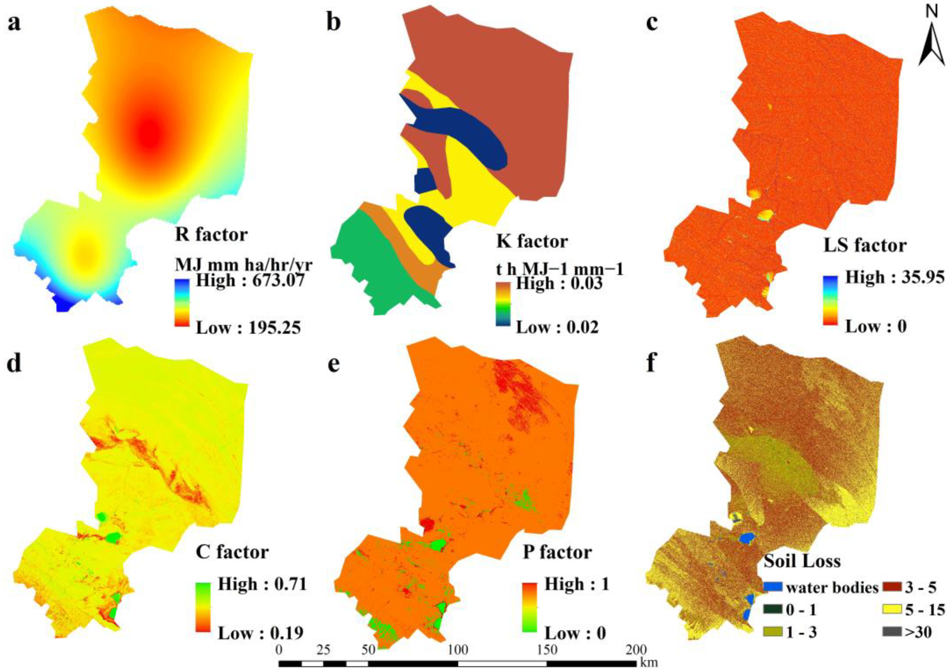
The utilization of the Revised Universal Soil Loss Equation (RUSLE) in arid and semi-arid environments might provide distinct outcomes that hold significance in comprehending and effectively addressing soil erosion in such areas [10,11,37]. Our examination of the existing state of soil erosion in the Talas area, employing the RUSLE model, has provided valuable insights into the magnitude and spatial distribution of erosional processes.

Central Asia is susceptible to the adverse effects of climate change, including heightened variability in precipitation, severe weather issues, and droughts [8,61]. Also, arid and semi-arid regions exhibit heightened susceptibility to soil erosion as a consequence of factors such as restricted plant coverage, irregular and strong precipitation patterns, and delicate soil characteristics [62]. The alterations in the magnitude and volume of precipitation are mostly influenced by the intricate mechanisms of the hydrological cycle inside the Earth’s atmosphere [17,61]. These modifications may lead to alterations in precipitation patterns, such as an increase in the intensity of rainfall events in some areas and the occurrence of lengthy periods of drought in others [18]. Precipitation patterns may also show seasonal and regional variations.

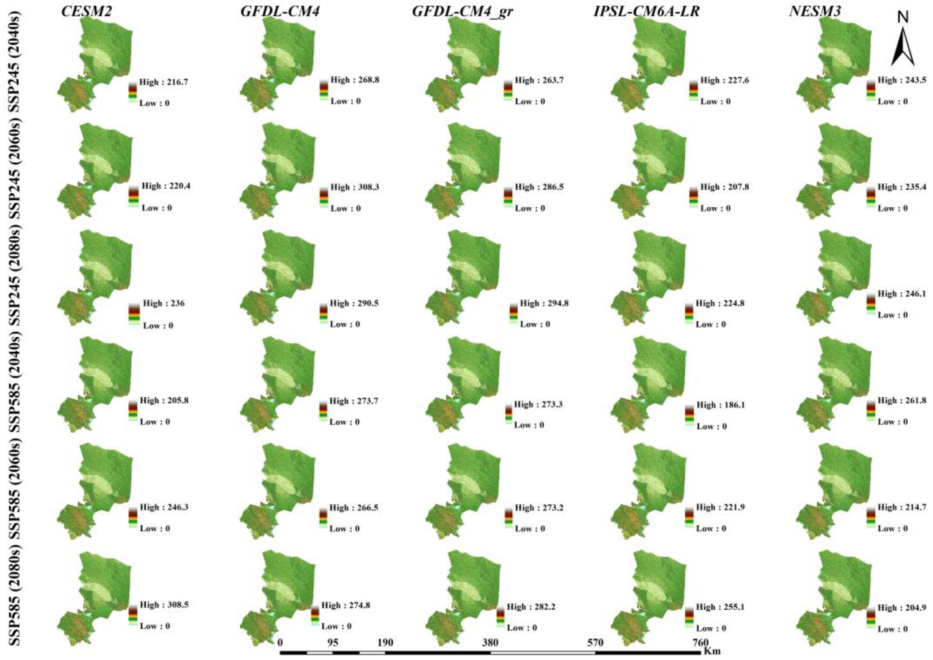
Areas with higher erosion risk can receive priority for re-vegetation or terracing, while areas with lower risk can be conserved as they are. The process of soil erosion modeling is inherently complex due to the geographical and temporal variability of soil loss, which is influenced by several elements and their intricate interrelationships. When making predictions about soil loss in unfamiliar areas, it is crucial to possess knowledge of both the estimations and the corresponding uncertainty.

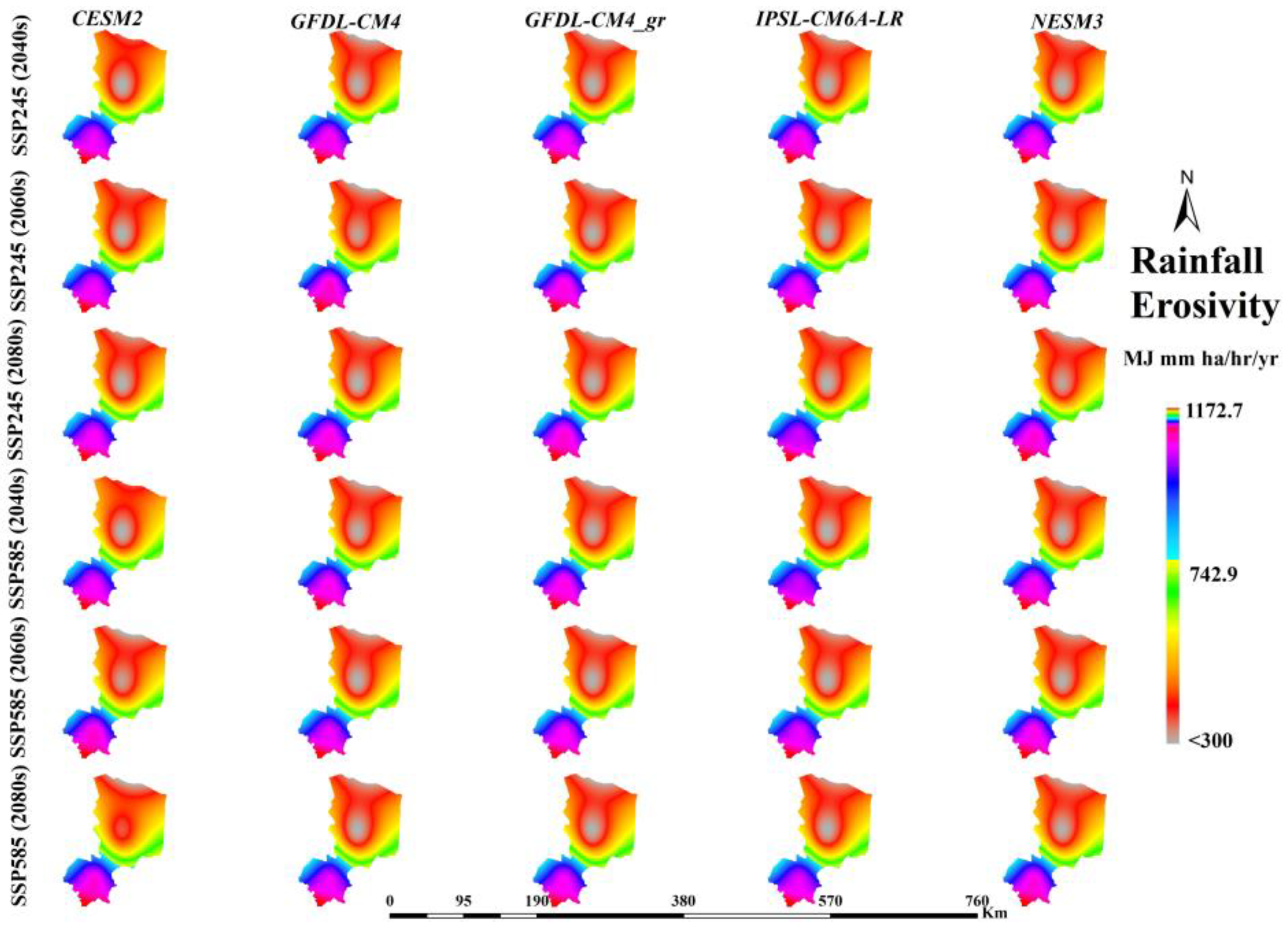
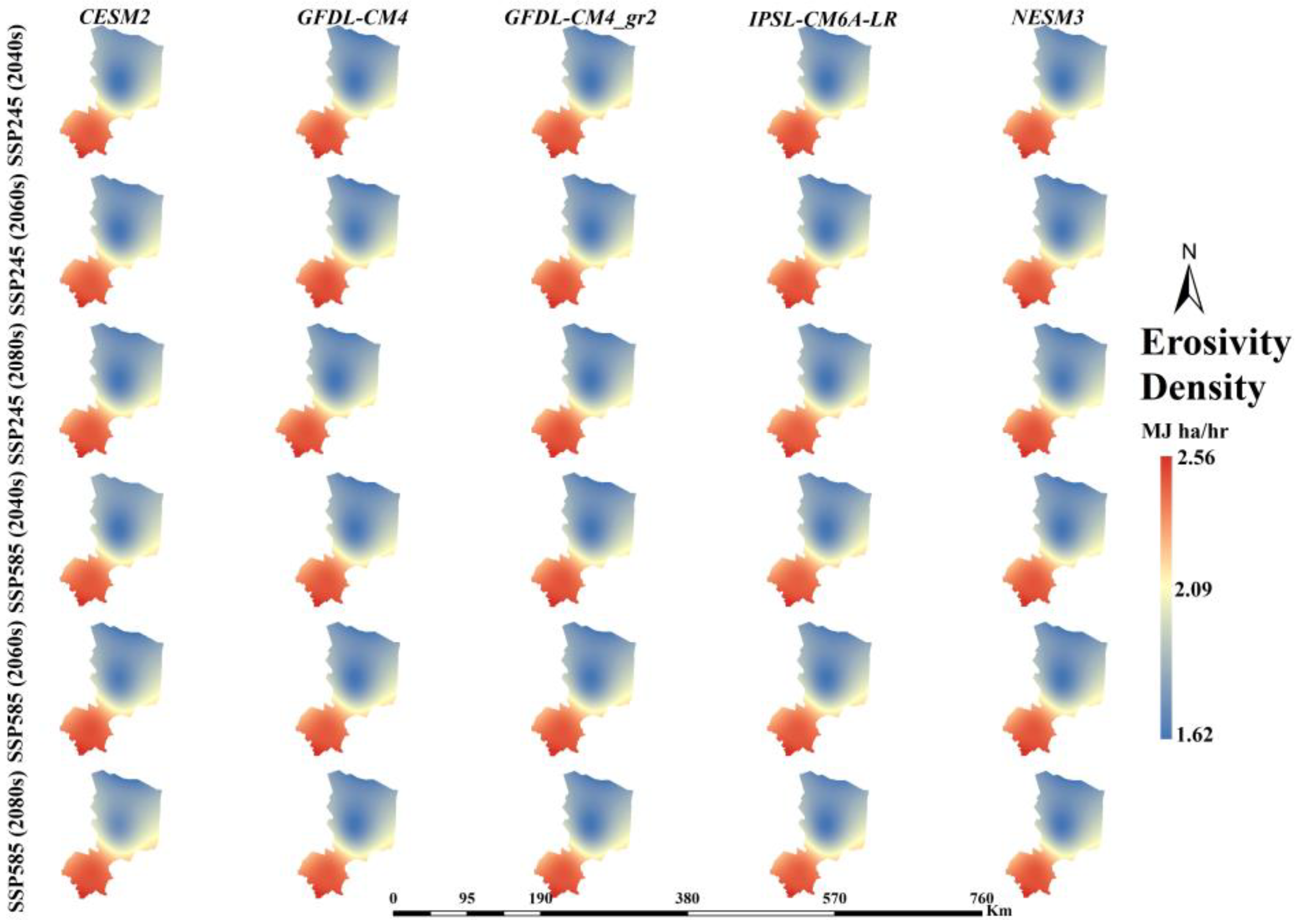
Multiple studies have shown that erosion densities beyond a value of 1 result in a higher occurrence of precipitation erosion compared with precipitation activity [59,60]. Rainfall erosivity, the power of rainfall to cause soil erosion, is an essential factor in soil erosion studies [63]. In the context of climate change, understanding and modeling the relationship between rainfall erosivity and shifting climate patterns is critical for effective soil conservation and land management. The findings of our research indicate that the subject region exhibits susceptibility to water erosion. The mean annual R coefficient demonstrated comparable values across various global climate models (GCMs). Consequently, the observed data values in the southern regions consistently rose. Various global studies consistently demonstrate an increase in rainfall throughout different time periods and geographical areas [64]. These fluctuations are probably associated with changes in the frequency and intensity of precipitation, rising temperatures, and changes in land use. This susceptibility to water erosion in the studied region underscores the importance of addressing the evolving climate patterns for sustainable soil conservation and land management practices. As climate change continues to exert its influence, understanding the intricate dynamics of rainfall erosivity becomes a cornerstone in developing effective strategies to mitigate soil erosion. The mean annual R coefficient, exhibiting comparable values across various global climate models (GCMs), adds a level of robustness to our findings. This consistency suggests that, despite variations in model outputs, there is a coherent trend in the susceptibility of the region to water erosion. Numerous studies have characterized and evaluated soil erosion in central Asia and our results coincide with the results of the above studies, specifically those by Duulatov et al. [11], Mukanov et al. [10], and Gafforov et al. [37], who conducted research at the central Asian scale.

The incorporation of climate projections from the CMIP6 GCM enhances the predictive capacity of our study. By integrating climatic data into the RUSLE model, we can simulate and anticipate potential alterations in soil erosion patterns under varying climatic scenarios. In our future research, hydrological models can be used to assess soil erosion under different land use types.

5. Conclusions

This study utilized observational data spanning 35 years and the RUSLE model with a combination of several GCMs to estimate soil erosion and evaluate the impact of various factors, including precipitation, soil characteristics, topography, land use, and conservation efforts, on erosion susceptibility in the Talas district. The findings indicate that the mean annual soil erosion rate observed over the study period ranges from 0 to 127 (t y⁻¹). Approximately 56.29% of the study area exhibits a low susceptibility to soil erosion, with an additional 33.56% classified as a moderate risk and 7.36% deemed at high risk of erosion. Additionally, the main general circulation models (GCMs) used for the SSPs 245 and 585 were evaluated, focusing on temporal spans for the near and far future—specifically, 2040 (2026–2050), 2060 (2051–2075), and 2080 (2076–2100). The assessment revealed a moderate increase in precipitation levels compared with the reference point, with predicted growth rates of 21.4%, 24.2%, and 26.4% for the years 2030, 2050, and 2070, respectively. Moreover, the research highlighted a positive correlation between soil erosion and precipitation, evidenced by a proportional increase in average erosion of 34%, 35.5%, and 38.9% during the respective time periods. The integration of the RUSLE and GCMs furnishes actionable insights, empowering scientists and stakeholders to make informed decisions regarding land management, conservation, and climate resilience.